www.geosci-model-dev.net/5/919/2012/ doi:10.5194/gmd-5-919-2012
© Author(s) 2012. CC Attribution 3.0 License.
Geoscientific
Model Development
MAESPA: a model to study interactions between water limitation,
environmental drivers and vegetation function at tree and stand
levels, with an example application to [CO
2
]
×
drought interactions
R. A. Duursma1and B. E. Medlyn2
1Hawkesbury Institute for the Environment, University of Western Sydney, Locked Bag 1797, Penrith, NSW 2751, Australia 2Department of Biological Sciences, Macquarie University, North Ryde, NSW 2109, Australia
Correspondence to: R. A. Duursma ([email protected])
Received: 8 December 2011 – Published in Geosci. Model Dev. Discuss.: 17 February 2012 Revised: 5 June 2012 – Accepted: 8 June 2012 – Published: 5 July 2012
Abstract. Process-based models (PBMs) of vegetation func-tion can be used to interpret and integrate experimental re-sults. Water limitation to plant carbon uptake is a highly uncertain process in the context of environmental change, and many experiments have been carried out that study drought limitations to vegetation function at spatial scales from seedlings to entire canopies. What is lacking in the synthesis of these experiments is a quantitative tool incor-porating a detailed mechanistic representation of the water balance that can be used to integrate and analyse experimen-tal results at scales of both the whole-plant and the forest canopy. To fill this gap, we developed an individual tree-based model (MAESPA), largely tree-based on combining the well-known MAESTRA and SPA ecosystem models. The model includes a hydraulically-based model of stomatal con-ductance, root water uptake routines, drainage, infiltration, runoff and canopy interception, as well as detailed radiation interception and leaf physiology routines from the MAES-TRA model. The model can be applied both to single plants of arbitrary size and shape, as well as stands of trees. The utility of this model is demonstrated by studying the inter-action between elevated [CO2] (eCa)and drought. Based on theory, this interaction is generally expected to be positive, so that plants growing in eCa should be less susceptible to drought. Experimental results, however, are varied. We apply the model to a previously published experiment on droughted cherry, and show that changes in plant parameters due to long-term growth at eCa (acclimation) may strongly affect the outcome ofCa×drought experiments. We discuss po-tential applications of MAESPA and some of the key uncer-tainties in process representation.
1 Introduction
The response of plant carbon uptake and water use to envi-ronmental change is complex because there are many interac-tions and feedbacks that modify the response to single envi-ronmental drivers. This complexity is highlighted by the re-markable diversity of experimental outcomes, for example in the response of plant water use and carbon uptake to elevated atmospheric [CO2] (Ainsworth and Long, 2005; Ainsworth and Rogers, 2007; Norby et al., 1999), warming (Rustad et al., 2001), and soil water deficit (Manzoni et al., 2011; Wu et al., 2011). Soil water availability frequently limits plant pro-ductivity, but because of interactions with plant properties, and with other environmental drivers, it remains difficult to predict the effect on vegetation water use and carbon uptake (Hanson et al., 2004). Because soil drought is already becom-ing more frequent as a result of climate change (Huntbecom-ington, 2006), it is crucial that its effect on vegetation function is more readily quantifiable.
experiments remains incompletely understood (Poorter and Navas, 2003). Meta-analyses usually focus on the effect of a single variable on vegetation function, although it has been recognized that interactions, feedbacks and acclimation are important in determining overall experimental outcomes (Norby and Luo, 2004; Norby et al., 1999; Wullschleger et al., 2002).
Typical experiments or long-term observations are con-ducted at spatial scales from whole plants (potted seedlings, whole-tree chambers) to entire canopies (eddy-covariance sites, free-air CO2 enrichment; FACE). A useful PBM to analyse and integrate experiments should therefore operate at both whole-plant and canopy scales. Another requirement is that the PBM incorporate detailed water balance routines and hydraulics of the soil-plant pathway.
Currently, no PBM exists that meets both requirements, and is sufficiently detailed to allow a connection with typical measurements of plant physiological function and plant canopy structure. Here, we introduce a new model, MAESPA, based on a combination of the well-known MAESTRA and SPA models.
The MAESTRA model is a tree array model that uses de-tailed radiative transfer calculations and leaf physiology to calculate radiation absorption, photosynthesis and transpira-tion of individual trees, growing singly or in a populatranspira-tion (Medlyn, 2004; Wang and Jarvis, 1990). The MAESTRA model has been applied in a wide range of contexts from hor-ticulture (e.g. Bauerle and Bowden, 2011) to regional climate change (e.g. Luxmoore et al., 2000), resulting in well over fifty publications (Medlyn, 2004; updated bibliography avail-able at www.bio.mq.edu.au/maestra/bibliog.html). A major limitation of this model, however, has been the lack of a dy-namic water balance. Medlyn et al. (2005) added the capac-ity to input soil moisture and thereby estimate the effect of a given soil moisture stress on photosynthesis and transpiration (e.g. as used by Reynolds et al., 2009), but the model does not calculate the soil moisture dynamically. This lack severely limits model applications in dry conditions because feed-backs to plant performance via soil moisture cannot be sim-ulated. For example, although the model has often been used to estimate effects of elevated atmospheric [CO2] (Ca)on canopy performance (e.g. Kirschbaum et al., 1994; Medlyn, 1996; Kruijt et al., 1999; Luo et al., 2001), the model can-not be used to investigate elevated [CO2] impacts in drought conditions because it is not possible to calculate how elevated [CO2] modifies soil moisture.
The SPA model (Williams et al., 2001a, b) is another well-known process-based model, with a focus on the im-pacts of water availability on forest canopies. However, this model is also limited in that it assumes a horizontally ho-mogenous canopy and thus does not allow for applications to individual trees. We added to MAESTRA the detailed soil water balance routines from the SPA model (Williams et al., 2001a, b), thus combining the strengths of the two models into a new soil-plant-atmosphere model that accounts
for non-homogenous stand structure. In addition, we made a number of improvements to the combined model that allow a detailed physiologically-based analysis of the complete soil-plant-atmosphere pathway. We believe that the new, com-bined model is a significant advance over either MAESTRA or SPA and will prove a useful tool for researchers in forest ecophysiology. Our goals in this paper are to fully document the new model and to demonstrate its use by applying it to a previously intractable question, namely the interaction be-tween atmospheric [CO2] (Ca)and drought.
Numerous experiments have been carried out on the inter-action ofCaand drought on plant functioning (see reviews by Rogers et al., 1994 and Wullschleger et al., 2002). A simple prediction for this interaction is that theCaresponse will be higher under soil drought for two reasons: firstly, lower leaf-level water use under eCa(Eamus, 1991; Medlyn et al., 2001) leads to higher soil water content, which helps plants avoid soil water deficits; and secondly, lower intercellular CO2 concentration (Ci)during drought enhances theCaresponse because of the non-linear response of photosynthetic rate to Ci (Grossman-Clarke et al., 2001; McMurtrie et al., 2008). While both mechanisms have been confirmed in a number of crop and grassland studies (e.g. Morgan et al., 2004; Rogers et al., 1994), experiments with potted tree seedlings, trees in whole-tree chambers or entire canopies in FACE experi-ments have yielded highly variable results (Gunderson et al., 2002; Nowak et al., 2004; Warren et al., 2010; Duursma et al., 2011). Two mechanisms are likely responsible for this variability in experimental outcomes: feedbacks from eCa -induced changes in plant size on water use and soil water bal-ance; and acclimation of leaf physiology to long-term growth at eCa. We first study the response of plant carbon uptake and water use to a simulated dry-down, which is a useful baseline for comparison with actual experimental outcomes. We then study the effects of acclimation of two leaf phys-iology parameters on theCa×drought interaction. Finally, we apply the MAESPA model to aCa×drought experiment where a feedback of increased leaf area in the eCatreatment confounds the direct effect ofCa, and show how analysis of experimental data within a model-based framework can ex-tend basic empirical results.
2 Methods
2.1 Model description
2.1.1 Overview
Weather
Tair, VPD (RH%), [CO2]
Radiation
Direct / diffuse, solar angle,PAR+NIR+LW
Canopy structure
Leaf area, crown size,
shape, leaf angle g ,
wavebands
Stomatal conductance model
Evaluated at each gridpoint in Extinction of radiation within
crowns + shading by neighbor trees (+scattering)
Incident PAR at leaf-level for each grid point
each gridpoint in the crown
Leaf photosynthesis model
Leaf-level CO2
assimilation (A), transpiration rates (E), leaf water potential () leaf water potential (L)
Fig. 1. Flowchart of MAESTRA, the above-ground model of the MAESPA model. Radiative transfer is calculated to a number of gridpoints (typically 72) in each target tree, which is used to drive the stomatal conductance and photosynthesis submodels. These leaf-level rates are then used to estimate whole-stand water use and carbon uptake (see Sect. “Total canopy transpiration”).
an early study on radiative transfer by Norman and Welles (1983), and solidified by Wang and Jarvis, (1990). Since then, many improvements have been made, in particular the leaf gas exchange calculations (Medlyn, 1996, 2004; Med-lyn et al., 2007), and the overall organization and dissemi-nation of the code (see http://www.bio.mq.edu.au/maestra/, hereafter referred to as “the MAESTRA website”). Our goal was to widen the applicability of the MAESTRA model by including detailed soil water balance routines and plant hy-draulic constraints on gas exchange.
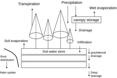
A basic overview of how MAESTRA estimates H2O and CO2exchange is given in Fig. 1. The processes included in the water balance sub-model are illustrated in Fig. 2. A full list of symbols is presented in Appendix A.
The MAESPA model, like MAESTRA and SPA, runs at typically a half-hourly time-step, although it can also be run at hourly or shorter arbitrary time-steps (up to every minute). 2.1.2 Canopy processes
Here, we provide a brief description of the canopy processes represented in MAESPA, which are largely unchanged from the original MAESTRA model (with the exception of stom-atal conductance). Our goal is not to provide an in-depth description of the entire MAESTRA model (see Wang and Jarvis, 1990; Medlyn, 2004; Medlyn et al., 2007 and the de-tailed manual on the MAESTRA website).
Deep drainage gravitational drainage
1 Soil water store
canopy storage Precipitation
Wet evaporation
Drainage
Infiltration Soil evaporation
Root distribution
Transpiration
Water uptake
Fig. 2. Flowchart of the water balance components of MAESPA, which are taken from the SPA model. The soil compartment is hori-zontally homogenous, and vertically divided into an arbitrary num-ber of layers.
Radiative transfer
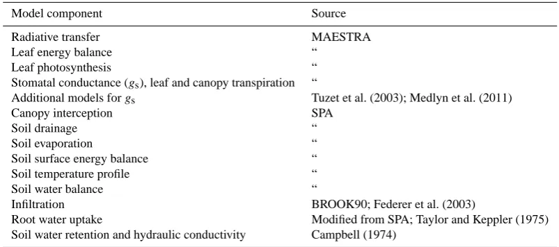
Table 1. Summary of origin of the various components of the MAESPA model. For the many references for the components of the MAESTRA model, see Sects. 2.1.1 and 2.1.2, and the MAESTRA website. For the components taken from SPA, see Williams et al. (2001a, b) for the sources of those components, or the corresponding sections in the main text.
Model component Source
Radiative transfer MAESTRA
Leaf energy balance “
Leaf photosynthesis “
Stomatal conductance (gs), leaf and canopy transpiration “
Additional models forgs Tuzet et al. (2003); Medlyn et al. (2011)
Canopy interception SPA
Soil drainage “
Soil evaporation “
Soil surface energy balance “
Soil temperature profile “
Soil water balance “
Infiltration BROOK90; Federer et al. (2003)
Root water uptake Modified from SPA; Taylor and Keppler (1975)
Soil water retention and hydraulic conductivity Campbell (1974)
calculated based on shading within the crown, shading by neighbouring trees, the location of the sun, and whether ra-diation is direct or diffuse. Scattering of rara-diation is approx-imated following Norman (1979). Leaf area within crowns is assumed to be distributed randomly, or to follow a beta-distribution in horizontal and/or vertical directions (Wang et al., 1990). At each grid point, leaf area is separated into sunlit and shaded leaf area (Norman, 1993), and the coupled stom-atal conductance – photosynthesis model is run separately for each fraction (Fig. 1).
Photosynthesis
For each grid point in the crown, leaf net photosynthesis is modelled using the standard model of Farquhar et al. (1980).
An=min Ac, Aj
−Rd (1)
whereAcis the gross photosynthesis rate when Rubisco
ac-tivity is limiting, Aj when RuBP-regeneration is limiting,
andRdthe rate of dark respiration.AcandAj are saturating
functions of the intercellular CO2concentration (Ci), both of the formk1(Ci-0∗)/(k2+Ci), where0∗ is the CO2 compen-sation point withoutRd, andk1andk2are different parameter combinations forAc andAj. The details of these functions
and the temperature dependence of the parameters are de-scribed elsewhere (e.g. Medlyn et al., 2002).
Stomatal conductance
For each grid point in the crown, leaf-level stomatal conduc-tance to H2O (gs)is modelled using a Ball-Berry type ap-proach (Ball et al., 1987) (Eq. 2).
gs=g0+g1An Cs
×f (D) (2)
whereAn is the leaf net assimilation rate (µmol m−2s−1), g0 the conductance when An is zero, g1 an empirical pa-rameter,f (D)a function of the leaf-to-air vapour pressure deficit (D)andCs the CO2concentration at the leaf surface (µmol mol−1)(which is corrected for boundary layer effects, but this is usually a small correction).
We have implemented a number of options for thef (D) function, including the Ball-Berry model (f (D)=1/RH, where RH is relative humidity) (Ball et al., 1987), the Le-uning model (f (D)=1/(1+D/D0)(Leuning, 1995), and the model of Medlyn et al. (2011), who showed thatf (D)= 1/
√
D follows from the assumption thatgs varies to main-tain δA/δE constant (cf. Cowan and Farquhar, 1977). The fourth option, which is used in the simulations shown in this paper, is a modified form of the Tuzet et al. (2003) model. This model takes into account the observation that the re-sponse of stomatal conductance toD and soil water deficit is controlled by the leaf water potential (9L)(Comstock and Mencuccini, 1998). Because 9L depends on the soil water potential (9S)as well as the transpiration rate (which
de-pends onD),9L summarizes the effect of bothD and9S
ongs (Franks, 2004). Tuzet et al. (2003) use a flexible9L modifier (in place of thef (D)function in Eq. 2),
f9L=
1+exp[sf9f]
1+exp[sf(9f−9L)]
(3) wheresf and9f are parameters; 9f is a reference water
potential, andsf is the “steepness” of the response off9Lto 9L. We assume a steady-state in water flow from the soil to the leaf, so that9L at the gridpoint can be calculated from Ohm’s analogy to water transport,
EL=kL(9S−9L) (4)
Sect. “Calculation of leaf temperature and leaf water poten-tial”), andkL the leaf-specific hydraulic conductance of the soil-to-leaf pathway (see Sect. “Hydraulics of the soil-to-leaf pathway”).
Finally, the coupled model ofgsandAcan be solved by using the basic diffusion equation,
An=gC(Cs−Ci) (5)
wheregC is stomatal conductance to CO2(=gs/1.6). The solution of the system of equations (Eqs. 1, 2 and 5) can be written as a quadratic equation, which yields theCi(see Wang and Leuning, 1998). We solve the Tuzet model (com-bination of Eqs. 2–5) numerically, by finding the9Lthat is the solution both to Eqs. (3) and (4). This way, a unique9L is calculated for each grid point in the crown. Variation be-tween trees arises due to shading effects, andkLis allowed to vary from tree to tree (as specified by the user). Also,kLis either assumed to be constant within the crown, or to follow a function of height above the ground as specified by the user. It should be noted that Tuzet et al. (2003) usedCiinstead of Ca in their model, but we useCa to be consistent with Medlyn et al. (2011), and to allow for much more straight-forward numerical model solution. The argument by Tuzet et al. (2003) to useCi instead ofCa is that stomata appear to respond toCi, notCa(Mott, 1988). However, we note thatCi is still implicit in Eq. (2), becauseAndepends onCithrough Eq. (1), andAnandgsare coupled byCithrough Eq. (5). Calculation of leaf temperature and leaf water potential
For the soil water balance, we use the Penman-Monteith equation applied at the canopy level (see Sect. “Total canopy transpiration”), to arrive at consistent calculations for stand energy balance, and boundary layer calculations for soil sur-face and canopy. At the leaf-level for each grid-point in the crown, transpiration (EL)is calculated to yield9Lthat is the solution to the Tuzet model of stomatal conductance (Eqs. 2 and 3), and to provide estimates of leaf temperature through-out the crown. For each grid point,ELis calculated with the Penman-Monteith equation (Eq. 6), which takes into account boundary layer effects on the exchange of water vapour be-tween leaves and the surrounding air. An iterative scheme is used that finds the leaf temperature that closes the energy balance of the leaf (following Wang and Leuning, 1998). Full details are provided in Medlyn et al. (2007).
Total canopy transpiration
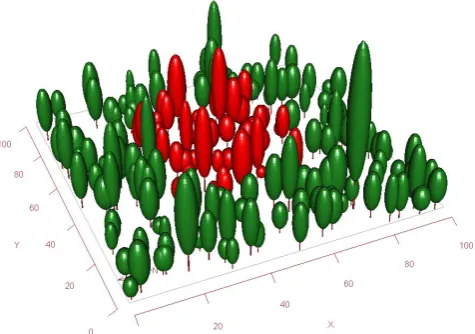
In MAESPA, the soil water balance is calculated using the spatially-averaged transpiration rate by the stand. This spatial average is calculated for a sample of trees specified by the user (the “target trees”), to limit computing time. An example of a selection of target trees is given in Fig. 3. We have chosen not to simulate spatial variation in soil water content based
Fig. 3. Example of a stand of trees as represented in the MAESPA model. Water use and carbon uptake are calculated for a sample of target trees, here shown in red, and then added to give the totals for the stand. It is recommended to select a set of target trees that are representative of the stand, and to account for edge effects.
on water uptake of the single trees in a stand, because such a model would be very difficult to parameterize and test.
This approach requires that we scale up estimates of tran-spiration to the stand level, and estimate total global (short-wave+longwave) radiation reaching the forest floor (for the soil heat balance calculations, see Sect. 2.1.4). Absorbed radiation (photosynthetically active radiation (PAR), near-infrared radiation (NIR) and thermal) is summed for each tree, and corrected for the difference in leaf area per tree for the sample trees, and that for the entire stand. Using the stand density, estimates of global radiation (W m−2) incident on the soil surface are obtained. Next, the average whole-tree conductance (mol tree−1s−1)is calculated across the sam-ple trees (weighed by their total leaf areas), and once again corrected for the difference in tree leaf area between sample trees, and the average tree in the entire stand. Stand transpira-tion is re-calculated using this average canopy conductance, and the intercepted radiation per tree, using the Penman-Monteith equation,
λET=sRn+DgBcpMa
s+γ gB/gV (6)
where λ the latent heat of water vapour (J mol−1), ET is canopy transpiration (mol m−2(ground) s−1),sthe slope of the relation between saturation vapour pressure and tempera-ture (Pa K−1), Rn net radiation (W m−2), gB the boundary layer conductance, and gV the total conductance to water vapour. The boundary layer conductance (gB, mol m−2s−1) for the canopy is calculated following Jones (1992),
gB= c×k
2 V×uz
[log((zH−zD)/z0)]2
wherekV von Karman’s constant,uz the wind speed
mea-sured at a height ofzH, andcconverts to molar units. The pa-rameterszDandz0are related to the extinction of wind speed above and within the canopy:z0is the “roughness length” re-lated to the roughness of the canopy surface, andzDis a ref-erence height. Both these parameters may be estimated from canopy height (Jones, 1992, p. 68), or from more detailed methods that account for stand structure (Schaudt and Dick-inson, 2000).
The total conductance to water vapour is,
gV=1/( 1 gC
+ 1 gB
) (8)
wheregC the canopy conductance (mol m−2s−1), which is estimated by averaging total conductance (mol tree−1s−1) across the sample trees weighed by their total leaf areas, and multiplying by stand density (m−2).
2.1.3 Water balance
Overview
The soil water balance is calculated for a horizontally ho-mogenous soil compartment, separated vertically in a num-ber of layers (typically ca. 10, specified by the user). The advantage of a multi-layer soil model is that the root density distribution can be specified, as well as vertical variation in soil texture. Furthermore, experiments have shown that plant water potential tends to equilibrate with the wettest zones in the soil, not the average soil water potential (Schmidhalter, 1997). Only a multi-layer soil model can reproduce this ob-servation.
In MAESPA, the soil water storage in each of the hori-zontally homogenous layers (si, mm) is calculated from
in-filtration (Ii), drainage (Di), root water uptake (Ei)and soil
evaporation (Es,i)(Eq. 9), at the same time-step as the
above-ground processes (typically, half-hourly). Soil evaporation draws water only from the top layer. Drainage out of the low-est root layer is defined as deep drainage.
dsi
dt =Ii−Ei−Di fori>1,and dsi
dt =Ii−Ei−Di−Es,ifor layer 1. (9) Infiltration
The rain that reaches the soil surface is assumed to infiltrate into more than just the top layer. This is accounting for rapid soil water flow through macropores (accounting for increases in soil water content at depth after heavy rainfall that cannot be accounted for by matric drainage rates). We use a sim-ple exponential function (taken from the BROOK90 model, (Federer et al., 2003) (Eq. 10).
Fori=1, Ii=Pu×(zi/Z)φ
Fori>1, Ii=Pu×
(
i X
1 zi)/Z
!φ
− (
i−1 X
1 zi)/Z
!φ
(10) whereφis an infiltration parameter (0-1),zi the depth to the
bottom of layeri(m), andZthe total soil depth (m). Ifφ= 0, all infiltration occurs in the top soil layer (no macropore flow). Ifφ=1, all layers receive equal infiltration.
Root water uptake
Total water uptake is distributed among soil layers accord-ing to the fine root density and soil water potential in those layers. The fraction of roots in each layer can be specified manually, or assumed to follow Eq. (11), which is useful be-cause Jackson et al. (1996) have summarized a large database on root distributions with this equation.
FR=(1−β100·zi)/(1−β100·Z) (11) whereFRis the cumulative fraction of fine roots to depthz (m), andβ is a parameter that specifies the shape of the dis-tribution (see Jackson et al., 1996). Soil depth is multiplied by 100, to be consistent with Jackson et al. (1996) who spec-ifiedzin cm. We have modified the original equation so that the total fine root length (an input parameter) is reached at the maximum depth of the rooting profile.
The root system can be viewed as a combination of re-sistances that are coupled in parallel, consisting of a soil-to-root surface resistance (Rsr)and a resistance to water uptake by the root itself (the radial resistance,Rrad). Because wa-ter transport is largely passive, following gradients in wawa-ter potential from soil to roots, the relative water uptake by dif-ferent layers in the soil follows from the partitioning of the resistances to water uptake in these layers. Generally, water uptake in a soil layer (Ei)is,
Ei=(9S,i−9R,i)/(Rsr,i+Rrad,i+Rlg,i) (12)
where9S,i is the soil water potential in layeri,9R,i is the
root xylem water potential, Rsr the soil-to root resistance, Rlgi the longitudinal resistance to water flow, andRrad the
radial resistance to water uptake (across the root epidermis to the xylem). This is a very difficult equation to solve simul-taneously for multiple soil layers, because9R,i,RradandRlg are typically unknown, and could vary with depth of the layer (especiallyRlg,i, as the path length through the root becomes
longer). To solve Eq. 12, we follow the assumptions by (Tay-lor and Keppler, 1975) who showed in an elegant experiment that (1)Rlgis very small compared toRrad, so that9R,i can
to the total fine root length in a soil layer, it follows that,
Ei ∝Lv,i 9S,i−9R (13)
where9Ris a mean root water potential, and Lv,i the fine
root density (m m−3)in layeri. The constant of proportion-ality may be found from the fact thatP
Ei=ET, whereET is the total water uptake. Note that we do includeRsr in the calculations of the overall resistance of the soil-to-leaf path-way (see Sect. “Hydraulics of the soil-to-leaf pathpath-way”), but omit it here to simplify the fractional uptake of water from different soil layers. The mean root water potential is taken as the minimum value allowed for roots (9Rmin), an input parameter; so that no uptake is possible in soil layers where the soil water potential is lower than9Rmin). When9R>9S, it is assumed that water does not flow from roots back into the soil, that is, we do not consider hydraulic redistribution in our model (see Domec et al., 2012).
Soil evaporation
The evaporation of water from the soil surface is estimated with a physical-based model developed by Choudhury and Monteith (1988), and modified by Williams et al. (2001a). Soil evaporation draws water only from the top layer, and assumes that water has to travel through a thin dry layer at the soil surface.
The rate of evaporation (mm) is determined from the dif-ference between water vapour pressure in the soil pore space and the air above, and a conductance to vapour transfer (Eq. 14),
Es=Gs,tk1(es−ea) (14)
whereGs,t is the total conductance from the soil air space to the air above the boundary layer (m s−1), ea the partial water vapour pressure of the air (kPa), andesthat of the soil pore space (kPa). The termk1converts from pressure units to volumetric units.Gs,tis the total conductance, including the path through the soil (Gws), and that through the boundary layer just above the soil surface (Gam). The latter is estimated following Eq. (7) (Sect. “Total canopy transpiration”), with the reference heightzD set to zero. Next,Gws is estimated from the diffusivity of water vapour, which is soil temper-ature dependent, and the tortuosity of the soil air pathway, which determines the effective path length for vapour trans-fer.
Gws=Deff(θ1/Ld) (15)
Deff=ωsθ1Dw (16)
whereDeffis the effective diffusivity,ωsa tortuosity
parame-ter,θ1the pore fraction of the top soil layer,Ldthe thickness of the dry layer at the soil surface, andDwdiffusivity of wa-ter vapour (calculated following Jones (1992) accounting for soil temperature). The rationale for Eq. (15) (Choudhury and
Monteith, 1988) is thatGwsis proportional to the air space in the soil, but inversely proportional to the distance water vapour has to travel. This distance is a function of both the thickness of the dry layer (Ld), and the tortuosity of the dry layer (Eq. 16).Lddepends on the timing of the last rainfall, and the rate of soil evaporation, but is not affected by plant water uptake. Following Williams et al. (2001b), MAESPA keeps track of multiple dry layers to account for complex dynamics with short intermittent storms. A minimum value (Ld,min)is specified as a parameter to prevent very high rates of soil evaporation in wet soil.
The partial pressure of water vapour in the soil pore space is calculated from,
es=esat×exp9s,1Vw/ (RTs) (17) whereesatis the saturated vapour pressure (calculated from temperature following Jones 1992),9s,1 the soil water po-tential in the surface layer,Vw the partial molal volume of water (m3mol−1),Rthe gas constant, andTsthe soil surface temperature (K).
Canopy interception
The Rutter et al. (1975) model of canopy rainfall interception is used. Rain has two possible fates: (1) it falls through the canopy without being intercepted or (2) it gets intercepted by the canopy, where it adds to a pool of canopy water, that slowly drains. If the maximum canopy pool is reached, all additional rainfall in that time-step drains immediately. Wa-ter also evaporates from the wet canopy, deWa-termined by the Penman-Monteith equation (see Sect. “Total canopy transpi-ration”), using infinite canopy conductance (because free wa-ter is available), but with VPD set to a very low value.
The change in canopy water storage (Wcan)is given by, dWcan
dt =(1−r1) P−Ew−e
r2+r3Wcan (18)
where Ew the wet evaporation rate (mm t−1), r1 the free throughfall fraction (0–1), andr2andr3are canopy drainage parameters. This differential equation is integrated with a Runge-Kutta method to obtain canopy throughfall, canopy storage, and wet evaporation rates.
Drainage
The vertical drainage of soil water is estimated directly from the soil hydraulic conductivity, which itself is a function of the soil water content. After adding the infiltration of rainfall to the soil water content for each layer, the water balance for each soil layer becomes,
dWi
dt =Di−1(θi−1)−Di(θi) (19) whereDi is the drainage from layeri. Because water is
solved for one layer at a time, starting at the top and mov-ing downward. Drainage is simply equal to the soil hydraulic conductivity (m s−1)in that layer, which is calculated from θi. The system of equations is solved with a Runge-Kutta in-tegrator (following the SPA model, Williams et al., 2001a, b).
Hydraulics of the soil-to-leaf pathway
We use the simple set of equations developed by (Campbell, 1974) for the dependence of soil water potential and the hy-draulic conductivity on the soil water content. Soil water po-tential (9S, MPa) is given by Eq. (20),
9s=9e
θ
θsat −b
(20)
whereθthe soil volumetric water content (m3m−3),θsatthe soil porosity, and9eandbare soil texture dependent
param-eters (see Cosby et al., 1984). Each of these paramparam-eters can vary by soil layer (isubscripts are omitted for clarity). The soil hydraulic conductivity is estimated from Eq. (21),
Ks(9s)=Ksat
9e 9s
2+3/b
(21)
where Ks the conductivity (mol m−1s−1MPa−1), 9e and b are the same parameters as in Eq. (20) (using the fact that conductivity and water potential are physically re-lated), and Ksat is the saturated hydraulic conductivity (mol m−1s−1MPa−1).
The soil-to-root resistance (MPa s m2(ground) mol−1)is estimated with the single root model of Gardner (1960) (see Williams et al., 2001a and Duursma et al., 2008 for more details). This model estimates the effective path length for water transport through the soil matrix to the root surface from the fine root density. The equation is,
Rsr,i=
log(rs
rr)
2π LVHsKs
(22) where rr the mean root radius (m), Lv the total fine root
density (m m−3)in the soil layer,Hs the height of the soil layer, and rs the mean distance between roots (1/
√ π LV). The total resistance for all soil layers combined (Rsr,t) is estimated by assuming that the resistances are coupled in parallel. The total leaf-specific hydraulic conductance (kL, mmol m−2(leaf) s−1MPa−1) from soil to leaf can now be found as,
kL=1/( 1
kP +Rsr,t×LT) (23)
where LT total canopy leaf area index
(m2(leaf) m−2(ground)), andkPthe plant component of the leaf-specific hydraulic conductance (mmol m−2s−1MPa−1), which is typically estimated from measurements ofEL and
9L under well-watered conditions (see, e.g. Delzon et al., 2004). It is assumed thatkPincludes the root components of the plant pathway (defined in Eq. 12 by the resistancesRrad andRlg), and that these components do not change with the plant water potential.
Following Williams et al. (2001a), we calculate a weighted soil water potential for use in the calculation of9Land stom-atal conductance. The9s in each layers is weighed by the
maximum water transport possible in that layer, depending on Rsr in that layer and a minimum root water potential (9R,min),
9S=
N P i=1
9S,i×Emax,i
N P i=1
Emax,i
whereEmax,i=(9S,i−9R,min)/Rsr,i.(24)
2.1.4 Soil heat balance
Overview
The components of the soil surface heat balance are calcu-lated to arrive at the soil surface temperature, and the vertical gradient of soil temperature. The soil surface temperature af-fects only the soil evaporation (see Sect. “Soil evaporation”). If soil evaporation is not of interest, or can be assumed neg-ligible, the soil heat balance need not be calculated (thereby simplifying the parameterization).
Soil surface temperature
The soil energy balance is the sum of four heat fluxes: net ra-diation (Qn), soil surface evaporation (latent heat flux) (Qe),
soil heat transport (to deeper soil layers) (Qc)and sensible
heat flux (Qh). Due to conservation of energy, these fluxes sum to zero at any time:
Qn+Qe+Qc+Qh=0. (25)
All the components in Eq. (25) depend on the soil sur-face temperature (Ts,1). The MAESPA model finds the soil surface temperature that provides closure in the soil energy balance.
Net radiation on the soil surface (Qn) is global radia-tion (solar+downward thermal) minus long-wave radiation (QL)emitted by the soil surface. The latter depends on the soil surface temperature (Eq. 26).
QL=εσ Ts4 (26)
where ε is the emissivity (assumed to equal 0.95), σ the Stefan-Boltzmann constant (W m−2K−4) and Ts is in K. Global down-welling radiation is the sum of short-wave ra-diation (i.e. solar rara-diation minus that intercepted by the canopy), and long-wave radiation emitted by the canopy.
The soil latent heat flux (Qe)is calculated from soil
Soil heat transport (Qc)follows from the difference in soil
temperature between the first and second layer,
Qc=Kth Ts,2−Ts,1/1z1,2 (27)
whereKthis the the soil thermal conductivity (W m−1K−1, see Sect. “Soil surface temperature”), and1z1,2 the depth difference between the second and first layer (m).
Sensible heat flux (Qh)is calculated from the difference between air temperature and soil surface temperature, and the total conductance to heat (Eq. 28)
Qh=cpρGa,m Ts,1−Tair (28)
wherecp the heat capacity of air (J kg−1K−1, a constant), ρthe (temperature-dependent) density of air (kg m−3),Ga,m the boundary layer conductance to heat transfer (assumed to be equal to that of water vapour transfer, see Sect. “Soil evap-oration”), andTs,1–Tairthe temperature gradient between soil surface and the air.
Soil temperature profile
The transport of heat down the soil temperature gradient is calculated following the SPA model (Williams et al., 2001b). The Fourier heat transport equation is solved using the Crank-Nichols scheme (Press et al., 1990) resulting in a soil temperature profile and corresponding heat fluxes be-tween soil layers. Inputs for this routine are the soil thermal conductivity (by layer), and soil heat capacity.
We used an empirical model developed by Lu et al. (2007) to estimate the soil thermal conductivity (in W m−1K−1) from soil porosity, water content, temperature and organic matter content. Their model takes slightly different parame-ter values for fine and coarse textured soils; we used the soil texture parameter (b in Eq. 20) to determine which param-eter set to use (based on their Table 1, we usedb=5.3 be-low which soils are considered “coarse textured”). With this method, it is straightforward to set the top layer of the soil as a “litter layer” that effectively insulates the soil through a very low thermal conductivity.
The heat capacity of the soil is determined by separating the soil into solid (quartz) and water fractions, and finding the weighted average of their heat capacities (cf. de Vries, 1963; see also Og´ee et al., 2001), and assuming that the soil air fraction has negligible heat capacity.
2.2 Parameterization
In MAESPA, the water balance is calculated for a horizon-tally homogenous soil, but the canopy consists of a collec-tion of single trees. Canopy transpiracollec-tion is estimated based on transpiration by the “sample trees”, and it is therefore vital that these sample trees represent the canopy in terms of water use. It is recommended that MAESPA is run for a large num-ber of sample trees, for example in an arrangement shown
in Fig. 3. For all trees in the stand, estimates of leaf area, crown shape, crown width, crown length and height to crown base are needed. Stands may also consist of just one tree, in which case the product of plot size and rooting depth can be interpreted as the soil volume, or pot volume, available to the tree.
Environmental drivers need to be specified on a (half-)hourly time-step, and include air temperature, solar ra-diation, precipitation, relative humidity and optionally wind speed and CO2concentration. For the water balance, crucial parameters are total rooting depth and the soil water reten-tion curve. The latter can be estimated from soil texture, and equations summarized by e.g. Saxton and Rawls (2006) and Cosby et al. (1984). A brief summary of the list of parame-ters needed to run the water balance component of MAESPA is given in Table B1.
2.3 Implementation and batch utility
MAESPA is written in Fortran, with simple text-based input and output files. An R (R Development Core Team, 2011) package is available, Maeswrap, which aides sensitivity anal-ysis and other computer-intensive simulation studies. This also includes a utility to graph the stand in 3-D (Fig. 3 was produced with the Maeswrap package). The compiled model and the source code are available on the MAESTRA website (see Sect. 2.1).
2.4 Application of MAESPA: a case study on the inter-action betweenCaand drought
In the following, we present three brief case studies that illus-trate the application of the MAESPA model to studying com-plex interactions between environmental drivers and plant parameters. All case studies analyse the interaction between atmospheric CO2concentration (Ca)and drought.
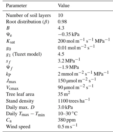
2.4.1 Dry-down simulations
Table 2. Important parameters for the simulation of a dry-down on daily whole-plant gas exchange and plant water relations. The soil type was a loamy sand (parameters from Cosby et al., 1984).
Half-hourly weather data were estimated from dailyTairamplitude.
Parameter Value
Number of soil layers 10
Root distribution (β) 0.98
B 4.3
9e −0.35 kPa
Ksat 200 mol m−1s−1MPa−1
g0 0.01 mol m−2s−1
g1(Tuzet model) 4.5
sf 3.2 MPa−1
9f −1.9 MPa
kP 2 mmol m−2s−1MPa−1
Jmax 150 µmol m−2s−1
Vcmax 90 µmol m−2s−1
Tree leaf area 35 m2
Stand density 1100 trees ha−1
Daily max.D 3.0 kPa
DailyTmax−Tmin 10–30◦C
Ca 380 ppm
Wind speed 0.5 m s−1
2.4.2 Effect of acclimation of leaf parameters onCa×
drought interaction in water use and CO2uptake
Acclimation of leaf physiology to long-term growth at eCa is one possible explanation for why many real-world exper-iments deviate from baseline expectations ofCa×drought interactions. We test the impact of acclimation of two leaf physiology parameters,kLand9f. A number of studies have
found decreases in the leaf-specific hydraulic conductance (kL)in plants grown in eCa(Atkinson and Taylor, 1996; Ea-mus et al., 1995; Eguchi et al., 2008; Heath et al., 1997), with reductions in a wide range of 10–100 %.
Berryman et al. (1994) found a higher sensitivity of gs to decreasing water content of excised leaves in Maranthes
corymbosa, which can be interpreted as a less negative9f in
the Tuzet model (Eq. 3). This observation is also consistent with a higher sensitivity to abscisic acid (ABA) in eCafound in a number of species (Dubbe et al., 1978; McAdam et al., 2011), and the fact that ABA concentrations increase in low 9L(Pierce and Raschke, 1981).
To test the sensitivity of theCa×drought interaction to these parameters, we ran two additional dry-down simula-tions, one with a 50 % reduction inkLat eCa, and one with a 0.4 MPa increase in9f. Both these changes in parameter
values are within observed ranges of change with long-term growth at eCa, but are arbitrary and only chosen to illustrate the effect on theCa×drought interaction. All other settings and parameters were as specified in the dry-down simulation (Sect. 2.2.1).
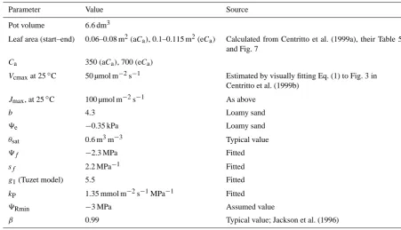
2.4.3 Drought×Cainteraction in cherry seedlings
To illustrate the importance of whole-plant feedbacks in treatment responses, we applied the model to aCa×drought experiment. Centritto et al. (1999a, b) describe an experiment where cherry seedlings were grown in ambientCa concentra-tion (aCa)(350 ppm) and elevatedCa(eCa; 700 ppm) treat-ments in well-watered conditions until half the plants were subjected to a dry-down. The analysis of their results was complicated by the fact that total leaf area of eCa seedlings was higher than that of aCa seedlings, compensating for lower water use per unit leaf area, so that total water use was similar between treatments. We re-analysed their dataset in a model-based framework where we can integrate effects of leaf area,Ca, and leaf-level physiology parameters on whole-plant interactions betweenCaand drought.
We estimated MAESPA parameters for the cherry seedling based on the published information as much as possible, and found the remaining parameters by fitting to observed data (see below). Details and estimated parameters are presented in Table 3. We constructed a weather dataset based on the lat-itude of the study and the reported mean air temperature and relative humidity. Daily incident PAR was estimated from air temperature using the Bristow and Campbell algorithm (Bristow and Campbell, 1984). Using the fitted parameter set for aCaplants, we simulated water use by the eCaplants, with the only difference that leaf area was increased as observed in the experiment.
3 Results
3.1 The interaction betweenCaand drought
A simulation was carried out to establish baseline behaviour of MAESPA during a dry-down.
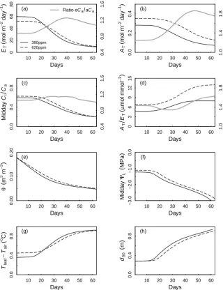
At ambient Ca, simulated total water use (ET)declines earlier and more rapidly than total carbon uptake (AT) (Fig. 4a and b), implying thatCi/Ca declines (Fig. 4c) and AT/ET increases as the dry-down progresses (Fig. 4d). As the soil water content declines (Fig. 4e), midday leaf water potential (9L)decreases steadily, and continues to decrease because of cuticular water loss (Table 2). Asgs decreases during the dry-down, the difference between leaf and air tem-perature increases (Fig. 4g), and the depth of water uptake gradually shifts to deeper layers (Fig. 4h).
10 20 30 40 50 60 0 20 40 60 80 Days ET ( m o l m − 2 d a y − 1 ) 0.4 0.8 1.2 1.6 380ppm 620ppm
RatioeCaaCa
(a)
10 20 30 40 50 60
0.0 0.2 0.4 Days AT ( m o l m − 2 d a y − 1 ) 1.0 1.4 1.8 (b) Days M id d a y Ci Ca
10 20 30 40 50 60
0.0 0.4 0.8 0.4 0.8 1.2 1.6 (c) Days AT ET ( µ m o l m m o l − 1 )
10 20 30 40 50 60
0 3 6 9 12 15 1.0 1.4 1.8 (d)
10 20 30 40 50 60
0.00 0.10 0.20 Days θ ( m 3 m − 3 ) (e)
10 20 30 40 50 60
−3.0 −2.0 −1.0 0.0 Days M id d a y ΨL ( M P a ) (f)
10 20 30 40 50 60
0.0 0.4 0.8 Days Tle a f − Ta ir ( o C ) (g)
10 20 30 40 50 60
0.0 0.4 0.8 Days d50 ( m ) (h)
Fig. 4. Simulation of the effect of a dry-down on whole-plant fluxes and water balance under ambient and elevatedCa. The simulation was
performed for a single tree with 35 m2leaf area in a stand of identical trees. Fluxes are expressed as averages over the canopy of that single
tree. See Table 1 for the parameter set used in the simulation. Shown are the decrease in total water use (ET), total daily net photosynthesis
(AT), middayCi/Ca, the daily integrated transpiration efficiency (AT/ET), volumetric soil water content (θ ), midday leaf water potential
for the sunlit leaves (9L), the difference between leaf and air temperature (Tleaf–Tair), and the depth of root water uptake (d50, the depth
above which 50 % of water is taken up). For panels (a)–(d), the ratio of eCato aCais shown with a grey line. Note the difference in scale for
this ratio (right y-axis) for panel (b).
a more pronounced increase inAT/ETas the drought pro-gresses (not shown). Both ET andAT show a three-phase response when expressed as the ratio eCato aCa(Fig. 4a and b). At first, when both plants have sufficient water, the ratio is constant. The ratio then increases due to higher soil water content in the eCatreatment. When this saved water store is exhausted (by day 40–45), the ratio declines, as bothETand ATare increasingly controlled by the cuticular conductance. MAESPA predicts a strong positive interaction between Ca and drought for two reasons. The first is the “water
Table 3. Important parameter settings for the simulation of theCa×drought interaction in cherry.
Parameter Value Source
Pot volume 6.6 dm3
Leaf area (start–end) 0.06–0.08 m2(aCa), 0.1–0.115 m2(eCa) Calculated from Centritto et al. (1999a), their Table 5
and Fig. 7
Ca 350 (aCa), 700 (eCa)
Vcmaxat 25◦C 50 µmol m−2s−1 Estimated by visually fitting Eq. (1) to Fig. 3 in
Centritto et al. (1999b)
Jmax, at 25◦C 100 µmol m−2s−1 As above
b 4.3 Loamy sand
9e −0.35 kPa Loamy sand
θsat 0.6 m3m−3 Typical value
9f −2.3 MPa Fitted
sf 2.2 MPa−1 Fitted
g1(Tuzet model) 5.5 Fitted
kP 1.35 mmol m−2s−1MPa−1 Fitted
9Rmin −3 MPa Assumed value
β 0.99 Typical value; Jackson et al. (1996)
0.00 0.05 0.10 0.15 0.20
0.0
0.5
1.0
1.5
2.0
θ (m3m−3)
R
a
ti
o
AT
(
e
Ca
)
/
AT
(
a
Ca
)
(a) No acclimationΨf+0.4 MPa
50%kP
0.00 0.05 0.10 0.15 0.20
0.0
0.5
1.0
1.5
2.0
θ (m3m−3)
R
a
ti
o
ET
(
e
Ca
)
/
ET
(
a
Ca
)
(b)
Fig. 5. Illustration of the influence of acclimation on the
interac-tion betweenCaand drought. Panel (a), relativeCaeffect on total
canopy CO2 uptake (AT)as a function of soil water content (θ )
during a simulated dry-down. Panel (b) shows total canopy
transpi-ration rate (ET)for the same simulations. The solid line shows the
interaction when all plant parameters are unchanged due to growth
at eCa(“no acclimation”). Note that in very dry soil, transpiration
rates are similar in aCa and eCa, but the stimulation of AT due
to eCa is much higher than in wet soil (a positive interaction of
drought and eCa). These effects are much reduced for a higher
sen-sitivity to9Lin the stomatal conductance model (“9f+0.4 MPa”),
which leads to a negative interaction betweenCaand drought (the
Caeffect is less in dry soil than wet soil, for bothETandAT). A
lower plant hydraulic conductance (kP)reducesETin wet soils, and
greatly reduces the positive interaction ofCaand drought that was
found without acclimation.
We studied the effect of acclimation of two leaf physiology parameters, the leaf-specific hydraulic conductance (kP)and the sensitivity to9L(9f, Eq. 3), on the “Ci effect”. When kP is reduced by 50 %, the strong positive interaction with soil water content as observed in the baseline simulation is much reduced (Fig. 5a), so that the eCa stimulation of AT is only moderately dependent on soil water content. When 9f is increased by 0.4 MPa, the interaction even reversed,
so thatATdecreases with eCain very dry soil (Fig. 5a) and ETis reduced by eCain very dry soil (Fig. 5b). This occurs because a higher9f leads to reduced stomatal conductance
(Fig. 6c), because9Lwas lower in the (simulated) eCa treat-ment.
Using the calibrated model, it is possible to tease apart contributions of different mechanisms on the overall inter-action betweenCaand drought, by running simulations with different settings. For this experiment, we ran simulations ex-ploring the contributions of changes in leaf area vs. changes in leaf-level water use. If plant leaf area was assumed un-changed between aCa and eCa treatments, we observed a very strong positive interaction between Ca and drought onET, as expected from the baseline simulations (Fig. 6c, dashed line). If leaf area was assumed to increase in the eCa treatment, but leaf-level water use was assumed not to change (dot-dashed line in Fig. 6c),ETdeclined much more quickly, indicating that the leaf-level response to eCadid have a sub-stantial ameliorating effect on the response ofETto drought. Finally, we quantified the drought impact on total pho-tosynthesis in the cherry experiment, by calculating total photosynthesis over the entire dry-down under different as-sumptions, and expressing it relative to simulated total pho-tosynthesis under well-watered conditions (Fig. 7). At aCa, drought reduced total photosynthesis by 22 %. For the eCa treatment, three simulations are summarized. The first two are calculated drought responses if leaf area is the same be-tween aCaand eCatreatments, and the third is the model pre-diction for the actual experimental conditions of the cherry experiment. The first simulation, Run 1, is the “baseline”, which includes both the “water savings” and the “Cieffect” (see above). The second simulation, Run 2, is at aCa, but with reduced leaf area to match the pre-drought eCa water use, and therefore is equivalent to the water savings effect of eCa. In the third simulation, Run 3, leaf area was increased similarly as in the cherry experiment, so that pre-drought water use was the same as in the aCa. In the eCa simula-tions, drought reduced total photosynthesis by 10 % (without feedbacks; Run 1), and 13 % (Run 2, water savings only), re-spectively. With the leaf area feedback (Run 3), there was a larger reduction in total photosynthesis (30 %), which coun-teracted the positive interaction betweenCaand drought. In summary, there was a positive eCa×drought interaction, be-cause drought reduced photosynthesis less in eCa than in aCa. This positive interaction was largely the result of the “water savings” effect, and disappears completely when leaf area is increased in eCa, as was the case in the cherry exper-iment.
4 Discussion
We have presented a new soil-plant-atmosphere model, MAESPA, that can be applied to both individual plant and whole stand scales. The model includes detailed radiation transfer and leaf physiology routines from the MAESTRA model, and mechanistic water balance and hydraulics from
● ● ● ● ● ● ● ● ● ● ● ● ● ● ● ● ● ●
0 10 20 30 40 50
0.0 0.1 0.2 0.3 0.4 0.5
Days into drought
θ ( m 3m − 3) Modelled aCa eCa ● ● Measured aCa eCa (a)
0 10 20 30 40 50
−3.0 −2.5 −2.0 −1.5 −1.0 −0.5 0.0
Days into drought
ΨL ( M P a ) ● ● ● ● ● ● ● ● ● ● ● ● ● ● ● ● ● ● (b)
0 10 20 30 40 50
0.0
0.5
1.0
1.5
Days into drought ET ( R a ti o e Ca a Ca ) Measured
Model:CaandAL
Model:Caonly
Model:ALonly
(c)
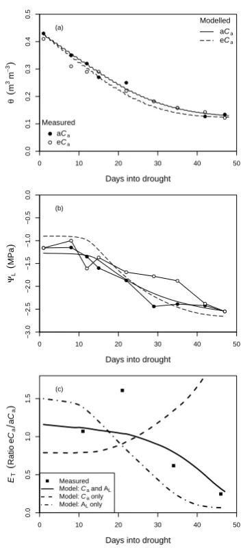
Fig. 6. Application of MAESPA to an experiment on droughted cherry seedlings by Centritto et al. (1999a, b). Model parameters were based on reported values in the original study, or calibrated to
yield a satisfactory fit to the data of the aCatreatment only (see text
and Table 2). The optimized parameter set was then used to
pre-dict water balance in the eCatreatment, and taking into account the
observed increase in leaf area in the eCaseedlings. (a) Decline in
average soil water content over the rooting zone (θ )as the drought
progressed. (b) Decline in the midday leaf water potential for sunlit
foliage (9L). Note a relatively poor fit for the eCatreatment:9L
is over-predicted early in the drought, and under-predicted towards
the end of the drought. (c) The ratio of total water use in eCa to
aCaduring the dry-down. Higher leaf area in eCainitially leads to
higher water use, but this leads to lowerθ(a) and9L(b), so that
eCaseedlings were more water-stressed toward the end of the
dry-down than their aCacounterparts. The solid line shows the
simula-tions where eCaand the increase in leaf area in the eCatreatment
were taken into account, dashed lines show either the directCa
ef-fect only (without leaf area feedback) or the leaf area feedback only
aCa Run 1 Run 2 Run 3
T
otal photosynthesis (r
atio droughted/irr
igated)
0.0
0.2
0.4
0.6
0.8
1.0
Ci
eff
ect + w
ater sa
vings
W
ater sa
vings only
Leaf area f
eedback
Fig. 7. Effect of the drought treatment on simulated total photosyn-thesis (summed over the entire 47 day simulation) for the dry-down
in the cherry experiment (Fig. 6). The aCasimulation shows a 22 %
reduction inATin the dry-down treatment. For eCa, three
simu-lations are shown. Run 1: full simulation but without the leaf area
feedback, Run 2: simulation at aCa, but with reduced leaf area to
match total water use in the eCasimulation (Run 1), Run 3:
includ-ing the observed leaf area increase in the eCatreatment.
the SPA model. We have shown that the model gives realis-tic predictions of the response of several plant variables to drought. As an example application, we used the model to study the interaction between atmospheric [CO2] (Ca) and drought.
4.1 Understanding controls on theCa×drought
interaction
In this paper, we illustrated the use of the MAESPA model by quantifying interactions between Ca and drought under several potential experimental scenarios. First we simulated our “baseline” expectation of theCa×drought interaction, in the absence of feedbacks or acclimation of plant proper-ties to long-term growth at eCa. Experimental outcomes can be compared to simulations like these, in order to evaluate whether the results are in quantitatively in line with current understanding of biophysical and physiological controls on whole-plant gas exchange and water balance.
The MAESPA model was able to simulate the effects of a soil dry-down on several variables in line with published ob-servations. During the dry-down,Ci/Casteadily decreased, so thatAT/ETincreased, which is consistent with published studies where non-stomatal limitations to carbon uptake are minimal (Brodribb, 1996). Midday leaf water potential (9L) decreased steadily, as typically observed (Sperry, 2000), and
leaf temperature increased as a result of lower stomatal con-ductance in dry soil (Jones, 1992; Triggs et al., 2004). Fi-nally, the depth of root water uptake gradually shifted to deeper layers (cf. Rambal, 1984; Duursma et al., 2011).
The baseline simulations predict that total CO2 uptake (AT)is enhanced more by eCa in dry soil (Fig. 5a), which is in line with previous predictions (Grossman-Clarke et al., 2001), and follows directly from the nonlinearity of the de-pendence ofAnonCi(the “Cieffect”). The magnitude of this drought-enhanced eCa response depends on the parameters used (in particularVcmax,g1), as well as the soil water con-tent (Fig. 5a). Although many studies on agricultural crops have demonstrated that biomass growth or net canopy car-bon uptake is more enhanced by eCaduring drought (Rogers et al., 1994), a great number of studies, particularly on trees, fail to demonstrate this effect (see Wullschleger et al., 2002; Nowak et al., 2004; Duursma et al., 2011; Warren et al., 2011). It should be noted that the interpretation of biomass growth in drought conditions is not straightforward because biomass growth may be temporally uncoupled from photo-synthetic CO2uptake (K¨orner, 2003; Sala and Hoch, 2009). However, this is unlikely an explanation for the lack of ob-servations for expectedCa×drought interaction in trees, be-cause many studies report CO2 uptake as well as biomass growth. We showed here that two plant parameters, that are frequently observed to be affected by acclimation to eCa, can reduce or even reverse this expected interaction (Fig. 6). Some studies have found this “reverse” response: Sch¨afer et al. (2002) found that, in a FACE study on Pinus taeda L.,EL was only reduced by eCawhen soil was dry, which counters the baseline expectation ofCaresponses (Fig. 6). In a FACE study on Liquidambar styraciflua L., Gunderson et al. (2002) found a higher sensitivity ofgs to9S in eCa trees, which also has the potential to reverse the expected interaction be-tweenCaand drought. We need to quantify the effect of such leaf acclimation to eCaand investigate the degree to which it can explain experimental outcomes that diverge from base-line predictions. A model such as MAESPA is an essential tool to quantify the contribution of such mechanisms.
ca. 50 % higher in the eCaplants. The MAESPA model suc-cessfully simulated the compensation of total plant water use by increased leaf area, using one parameter set for bothCa treatments, and the measured leaf areas. Because of the leaf area feedback, Centritto et al. (1999a) concluded that there was no positive interaction between drought andCa, a con-clusion that followed from a standard empirical analysis of the results. Experiments like this can be further analysed in a quantitative framework like MAESPA, because plant leaf area can be quantitatively accounted for in the simulations, which is much more difficult to accomplish in a purely em-pirical analysis. Using the parameterized model, it is then possible to separate the various contributing factors to the overallCa×drought interaction, and to estimate the strength of the interaction betweenCaand drought.
Using the parameterized MAESPA model, we showed that there were interactions betweenCaand drought in the cherry experiment. As the drought progressed, total plant water use declined more rapidly in the eCa treatment (Fig. 6c), an experimental observation that was roughly matched by the model simulation (Fig. 6c). However, a poor fit to9L (Fig. 6b) was necessary to match the larger reduction inET in eCaas the dry-down progressed (Fig. 6c). This mismatch is possibly because9Lwas sampled on a few sunlit leaves that were not representative of the entire canopy. Without the leaf area feedback, there was a strong simulated positive in-teraction ofCa and drought (Fig. 6c): water use could con-tinue much longer in the eCa treatment due to initial water savings. This analysis was therefore able to separate effects of leaf area and leaf-level processes on the response of plant water use to drought andCa.
The interaction betweenCaand drought is expected to par-ticularly affect plant CO2uptake (AT), because of the “Ci ef-fect”: photosynthesis is more responsive toCaat low stom-atal conductance, as is the case during drought (Fig. 5a). But what is the expected strength of this interaction, and is it more important than the “water savings” effect? For the cherry experiment, we calculated totalAT over the en-tire drying cycle, and expressed it as a ratio of droughted to irrigated control (Fig. 7). Drought reduced totalAT by a smaller fraction in the eCa treatment compared to the aCa treatment (10 % vs. 23 %). This relatively small difference is perhaps one reason that the Ca× drought interaction in experiments is often not significant, because there may be insufficient power to detect effects of this size. The simula-tion analysis demonstrated that the positive interacsimula-tion was mostly a water savings effect in this case, the “Cieffect” was very small (Fig. 7). It is possible that theCieffect is larger in other experiments, because it depends on the shape of theA– Cicurve, the degree of drought stress, stomatal conductance, and the length of the drought period.
Large scale simulations of Ca effects on vegetation wa-ter use and carbon uptake do not account for acclimation or feedbacks of plant processes to long-term growth atCa (e.g. Cramer et al., 2001; Luo et al., 2008), and as such yield
predictions of a positiveCa×drought interaction in line with the baseline predictions shown here (Fig. 4). However, actual experimental outcomes yield varied results, making it diffi-cult to inform model formulation and parameterization with experimental data. Here, we showed that by taking into ac-count the observed feedback of plant leaf area in one experi-ment, it is possible to study theCaeffect on plant water use and carbon uptake, had the feedback not occurred. A model like MAESPA can also be used to evaluate alternative expla-nations for the deviation from experimental outcomes from the expected theory, such as acclimation of plant hydraulic parameters (e.g.kP,9f), and to evaluate whether responses
at the leaf level match the responses at the whole-canopy scale.
4.2 Possible applications of MAESPA
While this study focussed on the interaction betweenCaand drought, there are a number of possible applications of a soil-plant-atmosphere model that can be applied to whole-plant and forest stand scales. Analysis of complex experiments where data are collected at leaf-level, whole-tree or canopy level, and in the soil, can be strengthened if all data are in-tegrated in the parameterization of a soil-plant-atmosphere model (Williams et al., 2001b; Medlyn et al., 2005; Duursma et al., 2007, 2009). Because MAESPA can be applied to pot-ted plants, it may be used to generalize experimental results from the vast number of experiments on potted plants, that are typically confounded by changes in plant size with ex-perimental treatments (e.g. Damesin et al., 1996).
There is a growing interest in the effects of stand structure on ecosystem functioning, because the spatial distribution of leaf area index (LAI) in sparse or dense crowns affects radi-ation interception, energy balance, and total water use (Chen et al., 2008; Yang et al., 2010), even though LAI is the pri-mary driver for fluxes of water and carbon. The MAESPA model is well suited to study effects of canopy structure and grouping of foliage in tree crowns on whole-canopy perfor-mance, and to evaluate simplified approaches.
All currently available soil-plant-atmosphere models can only be applied to entire canopies, restricting their use to studying stand-level processes. The advantage of MAESPA is that single plants can be studied. For example, models of vegetation water use are typically tested against scaled-up sap-flux measurements (Hanson et al., 2004; Williams et al., 2001a; Zeppel et al., 2008). An individual-based model such as MAESPA can be used to address questions of resource distribution among plants of different size and species within a canopy (cf. Binkley et al., 2010), in particular regarding the use of soil water and response to soil drought.
4.3 Uncertainty in process representation
improvements to models like MAESPA are certainly pos-sible. Below, we discuss uncertainty in three components of MAESPA, but they apply to any soil-plant-atmosphere model: root water uptake, variation in plant hydraulic con-ductance, and non-stomatal limitations to CO2uptake during drought. These three components are just examples where progress in process understanding will improve soil-plant-atmosphere models; there are certainly others.
Predicting the distribution of root water uptake with depth in the soil is an old problem (Gardner, 1964), and surpris-ingly little progress has been made since the simple model advanced by Taylor and Keppler (1975), which is used in nearly all root water uptake models (Feddes et al., 2001). Al-though this approach seems relatively successful in predict-ing relative uptake of water from different soil layers (Marke-witz et al., 2010), it is not useful in predicting the reduction in total water uptake when only a part of the root system is ac-cessing wet soil, as is the case for chronically droughted trees that have few roots at great depth (Calder et al., 1997). A bet-ter understanding of the root hydraulic conductance and how it varies with depth in the soil, and the partitioning of the re-sistance between radial and longitudinal components of the root pathway are needed to improve on this model compo-nent.
It is typically assumed, as in MAESPA, that the decline in CO2uptake during drought is the result only of reduced stomatal conductance, which simply limits the diffusion of CO2into leaves. However, there is ample evidence that pho-tosynthetic capacity (An at a given Ci) also declines dur-ing drought, albeit highly dependent on species and possibly only during more severe water stress (Lawlor and Cornic, 2002). Recently, Keenan et al. (2009) and Grant and Flana-gan (2007) both showed that accounting for the reduction in photosynthetic capacity with drought stress improved model predictions of canopy fluxes. A more general understand-ing of non-stomatal limitations and how they develop durunderstand-ing drought stress will improve models such as MAESPA.
In MAESPA, the hydraulic conductance of the plant path-way (kP)does not decline during drought, and does not vary among shaded or sunlit portions of the canopy. Although kP typically does decrease during drought due to formation of air-filled vessels (Sperry ,2000), Duursma et al. (2008) showed that a model assuming a fixedkP was successful in predicting the response of plant water use to water limitation, in part because the soil resistance becomes limiting to water transport (Fisher et al., 2006). Nonetheless, gradual reduc-tion inkP during drought is often an important determinant of plant water use (Sperry et al., 1998; Hacke et al., 2000).
Differences inkP between shaded and sunlit leaves in the canopy may exist because of shorter path length to shaded leaves, which increaseskPin shaded leaves relative to sunlit leaves (as assumed in the SPA model, Williams et al. ,1996), or more conductive tissues connecting sunlit leaves to the roots, which increases kP in sunlit leaves (Lemoine et al., 2002). It is advantageous for plants to increasekP to more
productive parts of the crown (Katul et al., 2003), but it is as yet unclear howkP actually varies within crowns. Recently, Peltoniemi et al. (2012) argued that it is optimal for plants to distribute total hydraulic conductance in a way thatkPis pro-portional to average PAR for any leaf in the canopy. If this hypothesis is confirmed with measurements, it greatly sim-plifies a difficult problem, and it can be readily implemented in MAESPA.
4.4 Conclusions
We have implemented a new tool to study single-plant or canopy-scale interactions between environmental drivers, canopy structure, weather, and soil water balance. The use-fulness of a single-tree model has already been demonstrated by the broad user-base of the MAESTRA model. Here, we have widened the applicability by introducing detailed water balance components, and hydraulic constraints on water use and CO2uptake. The new model incorporates a finer level of mechanistic detail than simplified water balance models (e.g. Granier et al., 1999), while still being relatively straight-forward to parameterize (see Table B1 for a list of required parameters for the water balance component).
We suggest a way forward in integrating diverse exper-imental results, by evaluating experexper-imental outcomes in a quantitative framework that summarizes our understanding of the soil-plant-atmosphere continuum. We showed that even relatively straightforward interactions like the Ca× drought interaction can be highly variable, because they are dependent on feedbacks of plant size on the soil water bal-ance and acclimation of plant properties due to long-term growth at Ca. Quantitative evaluation of the role of such feedbacks is essential if we are to advance our understand-ing of plant responses to environmental change. Too often in the current literature onCaexperiments, responses are sim-ply presented as significant/not significant, rather than being compared quantitatively to expectations based on current the-ory. As argued by Phillips and Milo (2009), we need to move from asking “Was there a change?” to asking “How large was the change, and is that what we expected?”
Appendix A
Table A1. List of symbols, their definition and units.
Model inputs and constants
Jmax Maximum rate of electron transport (µmol m−2s−1) Vcmax Maximum rate of Rubisco activity (µmol m−2s−1) IR Fraction inhibition ofRdin the light (–)
Ca Atmospheric CO2concentration (µmol mol−1)
γ Shape parameter of the light response of electron transport (–) g0gs whenAnis zero (residual stomatal conductance) (mol m−2s−1)
g1 Slope parameter of a Ball-Berry-type model ofgs(units depend on units off (D)) 9min Minimum leaf water potential (Ball-Berry model) (MPa)
9f 9Lwheref9L=0.5 (Tuzet model) (MPa) sf Steepness of thef9Lfunction (Tuzet model) (–)
kP Plant component of the leaf-specific hydraulic conductance (mmol m−2s−1MPa−1) uz Above-canopy wind speed (m s−1)
zH Measurement height of wind speed (m) z0 Roughness length (m)
zD Zero plane displacement (m) φ Infiltration parameter (–)
zi Soil depth to the bottom of layeri(m) Z Total soil depth (m)
β Root distribution parameter (–)
9Rmin Minimum root water potential (no uptake below this value) (MPa) ωs Tortuosity of the soil air space (–)
Ld,min Minimum thickness of the dry soil surface layer (m) Lv Fine root density (varies by soil layer) (m m−3) r1 Fraction throughfall of rain through canopy (–) r2,r3 Canopy drainage parameters (mm and –)
θsat Soil porosity (water content at saturation) (varies by layer) (m3m−3) Ksat Saturated soil hydraulic conductivity (varies by layer) (mol m−1s−1MPa−1) 9e Parameter for the soil water retention curve (MPa)
b Parameter for the soil water retention curve (–) rr Mean fine root radius (m)
LT Canopy leaf area index (m2m−2) Tair Air temperature (◦C)
Model variables, constants, and outputs
Ac Rubisco-activity limited gross leaf photosynthesis rate (µmol m−2s−1) Aj RuBP-regeneration limited gross leaf photosynthesis rate (µmol m−2s−1) An Net photosynthetic CO2uptake rate (µmol m−2s−1)
AT Total canopy CO2uptake rate (µmol m−2(ground) s−1) Rd Dark respiration (µmol m−2s−1)
Ci Intercellular CO2concentration (µmol mol−1) Cs CO2concentration at the leaf surface (µmol mol−1)
Q Photosynthetic photon flux density at the leaf level (µmol m−2s−1) J Electron transport rate (µmol m−2s−1)
0∗ CO2-compensation point in the absence of dark respiration (µmol mol−1) gs,gC Stomatal conductance to H2O (gs)and CO2(gc)(mol m−2s−1) 9L Bulk leaf water potential (MPa)
9S,i Soil water potential in soil layeri(MPa) 9R Mean root xylem water potential (MPa) D Leaf-to-air vapour pressure deficit (kPa)
kL Leaf-specific hydraulic conductance (mmol m−2s−1MPa−1) λ Latent heat of water vapour (J mol−1)
s The slope of the relation between saturation vapour pressure and temperature (Pa K−1) Rn Net radiation (W m−2)
gB Boundary layer conductance (mol m−2s−1) gV Total conductance to water vapour (mol m−2s−1) si Soil water storage in layeri(mm)
Ii Infiltration into layeri(mm) Di Drainage out of layeri(mm)
Ei Root water uptake (canopy transpiration) out of layeri(mm) Es Soil surface evaporation (mm)