www.geosci-model-dev.net/5/611/2012/ doi:10.5194/gmd-5-611-2012
© Author(s) 2012. CC Attribution 3.0 License.
Geoscientific
Model Development
The ACCENT-protocol: a framework for benchmarking and model
evaluation
V. Grewe1, N. Moussiopoulos2, P. Builtjes3,4, C. Borrego5, I. S. A. Isaksen6, and A. Volz-Thomas7 1Deutsches Zentrum f¨ur Luft- und Raumfahrt, Institut f¨ur Physik der Atmosph¨are, Oberpfaffenhofen, Germany 2Department of Mechanical Engineering of the Aristotle University Thessaloniki, Thessaloniki, Greece 3TNO Environment and Geosciences, Utrecht, The Netherlands
4Institut f¨ur Meteorologie, Freie Universit¨at Berlin, Germany
5Department of Environment an Planning, University of Aveiro, Portugal
6Center for International Climate and Environmental Research (CICERO), Oslo, Norway 7Institut f¨ur Energie- und Klimaforschung: Troposph¨are, Forschungszentrum J¨ulich, Germany Correspondence to: V. Grewe ([email protected])
Received: 28 November 2011 – Published in Geosci. Model Dev. Discuss.: 13 December 2011 Revised: 18 April 2012 – Accepted: 1 May 2012 – Published: 11 May 2012
Abstract. We summarise results from a workshop on “Model
Benchmarking and Quality Assurance” of the EU-Network of Excellence ACCENT, including results from other activi-ties (e.g. COST Action 732) and publications. A formalised evaluation protocol is presented, i.e. a generic formalism de-scribing the procedure of how to perform a model evaluation. This includes eight steps and examples from global model applications which are given for illustration. The first and im-portant step is concerning the purpose of the model applica-tion, i.e. the addressed underlying scientific or political ques-tion. We give examples to demonstrate that there is no model evaluation per se, i.e. without a focused purpose. Model eval-uation is testing, whether a model is fit for its purpose. The following steps are deduced from the purpose and include model requirements, input data, key processes and quanti-ties, benchmark data, quality indicators, sensitiviquanti-ties, as well as benchmarking and grading. We define “benchmarking” as the process of comparing the model output against either ob-servational data or high fidelity model data, i.e. benchmark data. Special focus is given to the uncertainties, e.g. in ob-servational data, which have the potential to lead to wrong conclusions in the model evaluation if not considered care-fully.
1 Introduction
Overview on the ACCENT model evaluation protocol
Purpose
What is the scientific or political question ?
Model requirements
What are the model requirements to answer the question ?
Input data
What data are necessary to run the model ?
Key processes / quantities
What are the key processes and quantities to be evaluated ?
Benchmark data
What observations or high fidelity model data are required for the validation ?
Quality indicators
How are model and observational data compared ?
Sensitivities
What model sensitivities have to be investigate to understand the robustness of the answers to the question ?
Benchmarking & Grading
What are the conclusions on the accuracy and robustness of the answer to the posed question, implied by the comparative analysis ?
Fig. 1. Overview on the ACCENT model evaluation protocol.
hence quality assurance, both for the benchmark data and the models is involved. In this paper we focus on a model eval-uation protocol in a generic form, which comprises previous model evaluations and summarises them as a framework and general strategy for future efforts. This protocol has emerged from an ACCENT-workshop on “Model Benchmarking and Quality Assurance”, held in Thessaloniki in 2006 (Mous-siopoulos and Isaksen, 2007), and is largely based on pre-vious activities (e.g. COST Action 723 “Quality Assur-ance of Microscale Meteorological Models”; http://www.mi. uni-hamburg.de/Home.484.0.html; Britter and Schatzmann, 2007a) and publications (Schlesinger et al., 1979; AIAA, 1998). Although the described protocol is generic and appli-cable to all scales, we focus on examples from global models for highlighting the different aspects.
The starting point of the protocol and every model evalua-tion is the formulaevalua-tion of its purpose, that is the overall scien-tific or political question which is aimed to be answered with the help of model simulations. Once this question has been clearly formulated, a number of implications for the evalua-tion follow, concerning the model itself, as well as the obser-vational data required and the comparative analysis. This is formulated as a framework, i.e. an evaluation protocol, which is outlined in Fig. 1 and discussed in more detail in Sect. 2.
2 The ACCENT model evaluation protocol
A brief overview on the ACCENT model evaluation protocol is given in Fig. 1, including 8 topics, which are briefly laid out with a question and more deeply described in the follow-ing sections.
2.1 The purpose of the evaluation
The most important issue and first step is to be clear about the purpose of the evaluation. What is the overall question that is aimed to be answered? The purpose of the evalua-tion has significant implicaevalua-tions on the details of the model evaluation. In the Introduction we have raised two ques-tions “Q1: When will the ozone layer recover?” and “Q2: How large is the climate impact from air traffic?”. Both top-ics are addressed by chemistry-climate models, however, the model requirements differ significantly. For example, the in-clusion of stratospheric polar clouds is a model requirement for question Q1, since they play an important role for the ozone hole (Crutzen and Arnold, 1986), whereas the forma-tion of contrail cirrus is a model requirement for quesforma-tion Q2 (Burkhardt and K¨archer, 2011). Noteworthy, the opposite is not true. Contrail cirrus are not regarded to be an impor-tant process for stratospheric ozone and polar stratospheric clouds are not relevant for subsonic air traffic. Hence, the set-up of a flexible or modular model will be chosen differently for these two purposes. Further, asking whether a model is good in the general sense is not as useful even not sensible as there are too many variables and aspects to assess.
Evidently, these examples show that a model evaluation necessarily requires a purpose, which implies that there is no general model evaluation per se.
2.2 The model requirements to fulfill the purpose
The identified purpose leads to a number of model require-ments for implemented processes, i.e. those related to the formation of polar stratospheric clouds for Q1 and the micro-physics of contrail cirrus for Q2. The implemented processes are, however, only part of the model requirements, which can be summarized by,
1. model description (including, name and contact infor-mation of person providing inforinfor-mation, version num-ber and release date of the model to ensure reproducibil-ity, a brief description of the intended use of the model, references);
2. necessary processes;
3. minimum (recommended) resolution (spatial and temporal);
4. minimum simulation set-up characteristics (domain, spin-up, simulation length, ensemble).
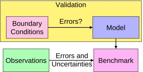
Validation
Errors?
Model
Boundary
Conditions
Benchmark
Observations
Errors and
Uncertainties
Fig. 2. Sketch of an intercomparison of modelling data to observa-tional data, illustrating the difficulties in attributing discrepancies to model deficiencies rather than input or boundary data uncertainties.
affected by the upper boundary of the modelling domain if chosen too close to the tropopause (Grewe et al., 2002). The spin-up time for models is closely related to the initial con-ditions. For example, simulating the evolution of the ozone hole (Q2) requires a correctly balanced situation, e.g. be-tween the emission of long-lived species (CFCs, N2O) and their concentrations.
2.3 The model input data
Generally, models and specifically climate-chemistry models require a large number of input parameters and (flux) bound-ary conditions, such as emissions, surface concentrations or sea-surface temperatures. The model output depends on these input parameters and boundary conditions and any validation necessarily addresses the combination of the input data and the model itself (Fig. 2). Taking stratospheric ozone as an example (Q1), Braesicke and Pyle (2004) and Garny et al. (2009) showed that the representation of sea surface tempera-tures have an impact on tropospheric and stratospheric ozone in the order of 10 %. The uncertainties in the input data give a limit to which a model can be evaluated. A discrepancy between model data and observational data hints at a model deficiency only if this discrepancy exceeds the model’s sen-sitivity to input data uncertainties. In many cases it is difficult to actually distinguish a model deficiency from a deficiency in the input data. Therefore, an evaluation protocol should include:
1. list of input data;
2. uncertainties of input data.
The sensitivities are important and hence covered separately in Sect. 2.7.
2.4 Key processes and quantities with respect to the purpose
A key part of the protocol is the description of the parame-ters, quantities or processes, which are important with respect
to the purpose of the evaluation. In many cases this part of the protocol is best documented and reviewed. Concerning the evolution of the ozone layer (Q1) a SPARC-activity (Strato-spheric Processes And their Role in Climate) was set-up to evaluate climate-chemistry models SPARC CCMVal (2010). A large number of quantities were identified and summarised in topics like radiation, dynamics, transport, stratospheric chemistry and microphysics.
There is a huge variety of possible parameters, e.g. tem-peratures, wind, ozone, nitrogen oxides, etc. and representa-tions of, e.g. long-term monthly means or medians, both for a region and for a certain altitude, seasonal cycles, variabili-ties, etc. This representation of the data is important, since the quality indicators and the benchmark depend on them (Sects. 2.6 and 2.8).
A further key aspect concerns the counterpart to the model data, namely the benchmark data used in the evaluation (Sect. 2.5). Generally the most favourable are observational data. However, high fidelity models are also frequently used, e.g. high resolution line-by-line radiation codes to evaluate radiative fluxes (SPARC CCMVal, 2010). In many cases ob-servational data are not available in the required representa-tion. It is important to indicate (a) why there is a need for these observational data, and (b) in case highfidelity model data is used, its range. Even without benchmark data, a model intercomparison still reveals the range of uncertainty and might foster research in this direction.
Therefore, the key parameters should be characterised by: 1. list of key parameters, quantities and processes; 2. representation;
3. description of benchmark data.
2.5 Benchmark data
As discussed in Sect. 2.4 the benchmark data, i.e. the data against which the model data are compared, are either obser-vational data or high fidelity model data. It is essential for the benchmarking (Sect. 2.8) to include all available quality information for the observational data, in order to provide a quantitative estimate of their overall uncertainty, including:
1. measurement techniques (accuracy and precision); 2. methodology;
3. representativity; 4. natural variablity.
more difficult to derive. Van Noije et al. (2006) have pre-sented results from a model intercomparison of tropospheric NO2 columns, in comparison to three different retrieval al-gorithms. Their results show that the spread between the model results is basically as large as the spread between the observational data. The inclusion of different retrieval algo-rithms provided an indication of the uncertainties associated with the methodology applied to the satellite data used as a benchmark. Without these uncertainties, the assessment of the model results would have been very different: Taking only the Bremen satellite data into account suggests that the models underestimate wintertime European NO2columns by a factor of two. However, taking all observational data into account leads to the conclusion that observational data and model data do not show any statistically significant differ-ence.
The representativity of the benchmark data is also a cru-cial point. For example in-situ measurements are often lo-cated at prominent locations, like mountain tops or at the sea side and are affected by the local environment. The lo-cal slo-cale of such observations makes it difficult to assure the representativity of the measurement for the grid box volume. Other aspects of representativity are associated with sam-pling methods (e.g. J¨ockel et al., 2010) and again retrievals. How accurate are height specifications of vertically resolved satellite data, i.e. how representative are satellite measure-ments for a certain height when the information is deduced from a column value and represents a certain height region? How representative are measurements of, e.g. tropospheric NO2 columns, when clouds shield a large fraction of lower tropospheric NO2? Richter and Burrows (2002) have inves-tigated these effects and showed that they can lead to poten-tially large uncertainties.
Another example are HALOE (Halogen Occultation Ex-periment; Russel III et al., 1993) satellite measurements of, e.g. HCl. Lary and Aulov (2008) showed a compari-son of frequency distributions of satellite HCl measurements for a height region in isentropic levels, and equivalent lati-tude bands representative for January conditions in the early 2000s. For some regions the difference between the indi-vidual measurement platforms was larger (up to 20 %) than the variability within one individual measurement platform, which shows that a bias can be significantly larger than the variability. Aghedo et al. (2011) compared chemistry-climate model output with satellite observations. This comparison was performed in two ways: (a) by comparing the model out-put directly with the satellite data and (b) by processing the model output in a way the satellite would have observed the model’s atmosphere (sampling, satellite processing). By the latter procedure they derived data which were based on ob-servational operators representing the satellite retrieval algo-rithms. They concluded that for most species the sampling would have a low error. However, in some cases neglecting observational operators has impacts for, e.g. ozone and water vapour on the order of 30 % and 100 %, respectively.
These examples show that uncertainties directly associated with the compilation of observational data, i.e. points (1) to (3) (see beginning of this section), severely impact the qual-ity aggregated data product. While this does not devaluate the data, it places great demands on the way the data are to be compared, i.e. the quality indicators used and their statis-tical interpretation (see Sect. 2.6). The determination of these uncertainties is indeed often challenging. However, to disre-gard the uncertainty rather than to use an educated guess or even a rough estimate is misjudging the consequences. Ne-glecting the uncertainties in the data implies the assumption of zero uncertainty, which is in general worse than using a rough estimate. For this reason, it is recommended to better rely on expert judgment than to disregard uncertainty.
The last point (4) is associated with natural variability and representativity of the data. If the targeted quantity is, e.g. a climatological mean mixing ratio for winter-time northern polar ozone at 50 hPa, a large interannual variability will lead to a large confidence interval for the climatological mean mixing ratio derived from the measurements, depending on sampling statistics. On the other hand, significant deviations between model and reality can only be claimed if the dif-ferences between model and observational data are large enough, e.g. the confidence intervals for the observational and model data are clearly separated. Again this is a mat-ter of the quality indicators (see Sect. 2.6) which, if chosen in a more appropriate way, might have reduced the statistical limitations.
A last point to mention is the need to provide a useful data format with respect to the uncertainty data. Certainly, two data types are required: First, meta data describing as a text the basis of the uncertainty estimate, which can range from “Expert judgement” to a short description of the algorithm and further reference. Second, the uncertainty in digital form in the same way as the measurement data itself.
2.6 Quality indicators
Quality indicators, i.e. the way model data and benchmark data are compared, have a large impact on the outcome of the evaluation. The list of possibilities is endless and ranges from a simple intercomparison of climatological mean val-ues to RMSE (root mean square error), NMSE (normalized mean square error), correlation coefficients, or so-called Tay-lor diagrams (TayTay-lor, 2001), which compare the normalised standard deviation versus the correlation coefficient. How-ever, there are requirements to the quality indicators, which mainly arise from the previous sections: quality indicators should:
1. resemble the representation of the key parameters (point 2 in Sect. 2.4);
3. include statistical tests on the significance of differences or
4. include confidence intervals for the quality indicators. Therefore, although there are many possibilities for qual-ity indicators, the definition of the key parameters, given in Sect. 2.4 largely constrains them. For example, if in Sect. 2.4 a seasonal cycle is identified as a key parameter, then a para-metric approach (Eq. 1) or the RMSE between deviations from the annual means (Eq. 2) can be taken into account.
f1(t )=asin(b t−c) (1)
f22=
12
X
i=1
(xmod(i)−xmodann)−(xobs(i)−xobsann)
2
(2) wheretis time,a,b,care parameters, which have to be fitted to either data set,xmod(i)andxobs(i)monthly mean values andxmodann andxobsann the respective annual means. In the first case differences in the fitted parametersa,b, andcbetween model and observational data would be the quality indicator and in the second case f2 is directly the quality indicator. The parametric approach f1 might provide more informa-tion, i.e. on amplitude, period and phase.
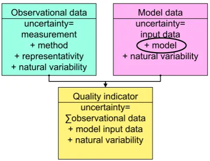
From the previous Sects. 2.3 and 2.5 it is clear that the use of the data, as they are, will very likely lead to misinterpre-tations, because the differences might arise from uncertain-ties in the data rather than from model deficiencies. Britter and Schatzmann (2007b) defined the total uncertainty of the model evaluation as a combination of uncertainties in the in-put data, benchmark data and natural variability (Fig. 3). This requires a calculation of confidence intervals or a statistical testing of the quality indicators. In the example above, this implies a test whether the fitted parametersa,b, andc dif-fer statistically significantly for the model and observational data. In the second example, a Monte-Carlo simulation could provide an uncertainty range and a confidence interval for
f2. This Monte-Carlo simulation replaces a complicated an-alytical calculation of the confidence interval and converts uncertainty ranges in the observational data into confidence interval for, e.g.f2.
2.7 Sensitivities
The application of the quality indicators including statistical tests allows one to infer which parameters are simulated with deficiencies. This has an impact on the quality with which the overall question, i.e. the purpose of the model (Sect. 2.1), can be answered. Hence, it is important to further under-stand these deficiencies and to provide a better underunder-standing of the simulated processes. This can be achieved by addi-tional simulations or diagnostics, which provide information on the sensitivity of the results to, e.g. input data. Again a wide range of examples exists in the literature. For exam-ple concerning the impact of air traffic on climate (Q2), the question of the contribution of other NOxsources (e.g. light-ning, Grewe, 2007) is of interest as well as the impact of
Observational data uncertainty= measurement
+ method + representativity + natural variability
Model data uncertainty=
input data + model + natural variability
Quality indicator uncertainty= ∑observational data
+ model input data + natural variability
Fig. 3. Sketch, showing the components of model and observa-tional data and the consequences for the uncertainties of the quality indicators.
model resolution and domain, feedbacks, and altitude of air-craft emissions (Grewe et al., 2002). A prominent difference between climate-chemistry models is the predicted methane and ozone response to air traffic emissions and especially their ratio (Lee et al., 2010). Stevenson et al. (2006) showed that although the methane lifetime was simulated very differ-ently by individual models, the sensitivity to different scenar-ios was very similar among the models, which provides more confidence in the sensitivities than the absolute numbers. Within the “Model and Measurement Intercomparison II” (Park et al., 1999), idealised air traffic emission simulations were performed to investigate the impact of mid-latitude air traffic emissions in comparison to high latitude emissions, in order to provide a basis for the robustness in simulating the effect of mid-latitude air traffic and to pin down differences in model results. Hence, a sensitivity analysis is a step be-yond an uncertainty assessment (Saltelli et al., 2000).
2.8 Benchmarking and grading
The evaluation protocol is a mixture of subjective choices and objective analysis. The choice of the key parameters and the corresponding quality indicator are based on expert knowledge and hence subjective. The analysis of the quality indicators itself is a mathematical procedure and hence ob-jective. A statistical test which includes the uncertainties in the data shows whether the model contradicts reality. A sta-tistical test which excludes uncertainties in the benchmark data only shows whether or not the model output contradicts the benchmark data (e.g. Grewe and Sausen, 2009).
Grade
Grade
Grade
Grade
Multi-model grades
Overall model grades
Statistics
Confidence
interval
Conf.
interval
=Benchmarking
Fig. 4. Overview on the whole benchmarking procedure.
acceptable range. The choice of this margin is again highly subjective and, in general, cannot be based on objective mea-sures.
Grading goes one step further by translating the outcome of the quality indicators and the margin into standardised units, e.g. a mark between 0 (bad) to 1 (excellent). Again the choice of the key parameter, the quality indicator, the margin and the grading formula are purely subjective, thus leading to pseudo-objective metrics. This is not devaluating grades, but has to be taken into account when comparing grades from, e.g. different model evaluations.
Moreover, grades can be and have been combined to multi-model grades (mean grade of many multi-models for one key rameter) or overall model grades (mean grade of all key pa-rameter for one model). Multi-model grades have the same basis, i.e. quality indicator and margin, and can be combined, whereas overall model grades are lacking a common basis, i.e. an ozone grade and a temperature grade are not compa-rable, which limits the interpretation of this metric. Hence, given the subjectivity of benchmarking, it is important that any assessment includes a clear description on how the as-sessment was conducted.
We have already stressed the importance of including a statistical test to the quality indicators in order to identify statistically significant differences between model prediction and reality deduced from benchmark data, and based on un-certainties in the model input data, measurement data and natural variability. It is a challenge to transfer this into a reli-able margin and grade. There is a substantial methodological difference between the mentioned test for quality indicators and for grades. The outcome of the test for quality indicators shows how much the model differs from the available bench-mark data, whereas grades include a much more quantitative aspect. The outcome of a test for grades includes, depending
on the grading formula, that the model differs from the real atmosphere by a certain distance to the margin. The test for the quality indicator is directly linked to the test whether a grade is 1, whereas for the grades the test for lower values than 1 has to be performed in addition. Grewe and Sausen (2009) have provided an example which transfers a widely used grading formula (Douglass et al., 1999; Kawa et al., 1999; Waugh and Eyring, 2008; SPARC CCMVal, 2010) into a statistically tested grading formula by calculating confi-dence intervals for the quality indicators and then using its lower bound as a new margin for grading. Their results show that without such a transformation the grading results cannot be interpreted in a reasonable manner. To summarise, bench-marking and grading requires:
1. definition of a margin, within which quality indicators are indicating acceptable model results;
2. definition of a grading formula, which represents a sta-tistical significant difference of model results from the margin and takes into account an estimate of the reality deduced from observations.
3 Summary
The aim of this study is to provide a framework for model evaluation, i.e. a model evaluation protocol. It was prepared during an ACCENT workshop held in Thessaloniki in May 2006 (Moussiopoulos and Isaksen, 2007) and further refined afterwards. Hence this protocol is based on input from a broad community including experts from observational and modelling communities, and covering expertise from local, regional and global aspects.
political question, which is aimed to be answered by the modelling activity. Other issues, like model requirements, model input data, key parameters and processes, etc., can then be deduced from the purpose, though subjectively based on expert knowledge.
It is important to stress the role of uncertainties in the eval-uation. Britter and Schatzmann (2007b) defined the total un-certainty of quality indicators as a combination of uncertain-ties in the input data, benchmark data and natural variability. The uncertainties in the benchmark data or observational data are crucial and include uncertainties of the measurements, the uncertainty in the methodology used for conversion of a measured physical quantity into the targeted atmospheric quantity, and the representativity of the observational data for the modelling counterpart (spatial/temporal representativity). Disregarding any of these uncertainties implies the assump-tion of a zero uncertainty and, hence, an expert judgment of the uncertainties should be used if independent information is not available.
The benchmarking itself, i.e. the quantitative comparative analysis with respect to a reference value, has to include sta-tistical tests to ensure that the uncertainties of the quality in-dicator are not leading to misjudgment of the model perfor-mance.
As a result, two main conclusions can be formulated. A model evaluation demands the purpose of the model applica-tion and uncertainties in the benchmark data have to be in-cluded to be able to deduce a statistical significant deviation of the model from reality.
Acknowledgements. This work was supported by the Network of Excellence ACCENT and the DLR-project ESMVal.
Edited by: S. Easterbrook
References
ACCENT (Atmospheric Composition Change the European Net-work of Excellence): Answers to the Urbino Questions, AC-CENTs first policy-driven synthesis, edited by: Raes F. and Hjorth J., published by: ACCENT Secretariat, University Urbino, Italy, ISBN 92-79-02413-2, http://www4.nilu.no/portal/ publications/accent-series-reports, 2006.
ACCENT (Atmospheric Composition Change the European Net-work of Excellence): Editorial, edited by: Fuzzi, S. and Maione, M., Atmos. Environm., 43, 5136–5137, 2009.
Aghedo, A. M., Bowman, K. W., Shindell, D. T., and Faluvegi, G.: The impact of orbital sampling, monthly averaging and vertical resolution on climate chemistry model evaluation with satellite observations, Atmos. Chem. Phys., 11, 6493–6514, doi:10.5194/acp-11-6493-2011, 2011.
AIAA (American Institute of Aeronautics and Astronautics): Guide for the Verification and Validation of Computational Fluid Dy-namics Simulations, American Institute of Aeronautics and As-tronautics, AIAA-G-077-1998, Reston, VA, USA, 1998.
Braesicke, P. and Pyle, J.: Sensitivity of dynmaics and ozone to dif-ferent representations of SSTs in the Unified Model, Q. J. Roy. Meteor. Soc., 130, 2033–2045, 2004.
Britter, R. and Schatzmann, M.: Model evaluation guidance and protocol document, COST Action 732, 28 pp., ISBN 3-00-018312-4, Hamburg, Germany, 2007a.
Britter, R. and Schatzmann, M.: Background and justification doc-ument to support the model evaluation guidance and protocol, COST Action 732, p. 88, ISBN 3-00-018312-4, Hamburg, Ger-many, 2007b.
Burkhardt, U. and K¨archer, B.: Global radiative forcing from con-trail cirrus, Nature Climate Change, 1, 54–58, 2011.
Crutzen, P. J. and Arnold, F.: Nitric acid cloud formation in the cold Antarctic stratosphere: a major cause for the springtime “ozone hole”, Nature, 324, 651–655, 1986.
Douglass, A. R., Prather, M. J., Hall, T. M., Strahan, S. E., Rasch, P. J., Sparling, L. C., Coy, L., and Rodriguez, J. M.: Choosing mete-orological input for the global modeling initiative assessment of high-speed aircraft, J. Geophys. Res., 104, 27545–27564, 1999. Garny, H., Dameris, M., and Stenke, A.: Impact of prescribed SSTs
on climatologies and long-term trends in CCM simulations, At-mos. Chem. Phys., 9, 6017–6031, doi:10.5194/acp-9-6017-2009, 2009.
Grewe, V.: Impact of climate variability on tropospheric ozone, Sci. Total Environ., 374, 167–181, 2007.
Grewe, V. and Sausen, R.: Comment on “Quantitative performance metrics for stratospheric-resolving chemistry-climate models” by Waugh and Eyring (2008), Atmos. Chem. Phys., 9, 9101– 9110, doi:10.5194/acp-9-9101-2009, 2009.
Grewe, V., Dameris, M., Fichter, C., and Sausen, R.: Impact of aircraft NOx emissions. Part 1: Interactively coupled climate-chemistry simulations and sensitivities to climate-climate-chemistry feedback, lightning and model resolution, Meteorol. Z., 3, 177– 186, 2002.
J¨ockel, P., Kerkweg, A., Pozzer, A., Sander, R., Tost, H., Riede, H., Baumgaertner, A., Gromov, S., and Kern, B.: Development cycle 2 of the Modular Earth Submodel System (MESSy2), Geosci. Model Dev., 3, 717–752, doi:10.5194/gmd-3-717-2010, 2010. Kawa, S. R., Anderson, J. G., Baughcum, S. L., Brock, C. A., Brune,
W. H., Cohen, R. C., Kinnison, D. E., Newman, P. A., Rodriguez, J. M., Stolarski, R. S., Waugh, D., and Wofsy, S. C.: Assessment of the Effects of High-Speed Aircraft in the Stratosphere: 1998, NASA-Report, NASA/TP-1999-209237, 1999.
Lary, D. J. and Aulov, O.: Space-based measurements of HCl: Intercomparison and historical context, J. Geophys. Res., 113, D15S04, doi:10.1029/2007JD008715, 2008.
Lee, D. S., Pitari, ,G., Grewe, V., Gierens, K., Penner, J. E., Petzold, A., Prather, M. J., Schumann, U., Bais, A., Berntsen, T., Iachetti, D., Lim, L. L., and Sausen, R.: Transport impacts on atmosphere and climate: Aviation, Atmos. Environm. 44, 4678–4734, 2010. Moussiopoulos, N. and Isaksen, I.: Proceedings of the
Workshop on Model Benchmarking and Quality As-surance,ACCENT Series Reports 2.2007, 60 p., http: //www4.nilu.no/farcry accent/download.cfm?DownloadFile= 3DCD0697-17A4-8DB2-8C63CCDF7478BCB6, 2007. Park, J. H., Ko, M. K. W., Jackman, C. H., Plumb, R. A., Kaye, J.
Parrish, D. D., Millet, D. B., and Goldstein, A. H.: Increasing ozone in marine boundary layer inflow at the west coasts of North America and Europe, Atmos. Chem. Phys., 9, 1303–1323, doi:10.5194/acp-9-1303-2009, 2009.
Penner, J. E., Lister, D. H., Griggs, D. J., Dokken, D. J., and McFar-land, M.: Aviation and the Global Atmosphere. A special report of IPCC Working Groups I and III, 373, Cambridge Univ. Press, Cambridge, UK, 1999.
Richter, A. and Burrows, J. P.: Tropospheric NO2from GOME mea-surements, Adv. Space Res., 29, 1673–1683, 2002.
Russell III, J. M., Gordley, L. L., Park, J. H., Drayson, S. R., Hes-keth, D. H., Cicerone, R. J., Tuck, A. F., Frederick, J. E., Harries, J. E., and Crutzen, P.: The Halogen Occultation Experiment, J. Geophys. Res., 98, 10777–10797, 1993.
Saltelli, A., Chan, K., and Scott, E. M.: Sensitivity Analysis, John Wiley & Sons, Chichester, New York, 2000.
Schlesinger, S., Crosbie, R. E., Gagn´ne, R. E., Innis, G. S., Lalwani, C. S., Loch, J., Sylvester, R. J., Wright, R. D., Kheir, N., and Bartos, D.: Terminology for Model Credibility, Simulation, 32, 103–104, 1979.
Stevenson, D. S., Dentener, F. J., Schultz, M. G., Ellingsen, K., van Noije, T. P. C., Wild, O., Zeng, G., Amann, M., Ather-ton, C. S., Bell, N., Bergmann, D. J., Bey, I., Butler, T., Co-fala, J., Collins, W. J., Derwent, R. G., Doherty, R. M., Drevet, J., Eskes, H. J., Fiore, A. M., Gauss, M., Hauglustaine, D. A., Horowitz, L. W., Isaksen, I. S. A., Krol, M. C., Lamarque, J.-F., Lawrence, M. G., Montanaro, V., M¨uller, J.-F., Pitari, G., Prather, M. J., Pyle, J. A., Rast, S., Rodriguez, J. M., Sanderson, M. G., Savage, N. H., Shindell, D. T., Strahan, S. E., Sudo, K., and Szopa, S.: Multimodel ensemble simulations of present-day and near-future tropospheric ozone, J. Geophys. Res., 111, D08301, doi:10.1029/2005JD006338, 2006.
SPARC Report on the Evaluation of Chemistry-Climate Models: SPARC Report No. 5, edited by: Eyring, V., Shepherd, T. G., and Waugh, D. W., WCRP-132, WMO/TD-No. 1526, http://www. atmosp.physics.utoronto.ca/SPARC, 2010.
Taylor, K. E.: Summarizing multiple aspects of model performance in a single diagram, J. Geophys. Res., 106, 7183–7192, 2001. van Noije, T. P. C., Eskes, H. J., Dentener, F. J., Stevenson, D. S.,
Ellingsen, K., Schultz, M. G., Wild, O., Amann, M., Atherton, C. S., Bergmann, D. J., Bey, I., Boersma, K. F., Butler, T., Co-fala, J., Drevet, J., Fiore, A. M., Gauss, M., Hauglustaine, D. A., Horowitz, L. W., Isaksen, I. S. A., Krol, M. C., Lamarque, F., Lawrence, M. G., Martin, R. V., Montanaro, V., M¨uller, J.-F., Pitari, G., Prather, M. J., Pyle, J. A., Richter, A., Rodriguez, J. M., Savage, N. H., Strahan, S. E., Sudo, K., Szopa, S., and van Roozendael, M.: Multi-model ensemble simulations of tro-pospheric NO2 compared with GOME retrievals for the year 2000, Atmos. Chem. Phys., 6, 2943–2979, doi:10.5194/acp-6-2943-2006, 2006.
Waugh, D. W. and Eyring, V.: Quantitative performance met-rics for stratospheric-resolving chemistry-climate models, At-mos. Chem. Phys., 8, 5699–5713, doi:10.5194/acp-8-5699-2008, 2008.