A generic biogeochemical module for Earth system models: Next Generation BioGeoChemical Module (NGBGC), version 1.0

(1)

www.geosci-model-dev.net/6/1977/2013/ doi:10.5194/gmd-6-1977-2013

Geoscientific

Model Development

A generic biogeochemical module for Earth system models:

Next Generation BioGeoChemical Module (NGBGC), version 1.0

Y. Fang1, M. Huang2, C. Liu3, H. Li1, and L. R. Leung2

1_{Hydrology Group, Energy and Environment Directorate, Pacific Northwest National Laboratory, Richland, WA 99352, USA} 2_{Climate Physics Group, Fundamental and Computational Sciences Directorate, Pacific Northwest National Laboratory,} Richland, WA 99352, USA

3_{Geochemistry Group, Fundamental and Computational Sciences Directorate, Pacific Northwest National Laboratory,} Richland, WA 99352, USA

Correspondence to: Y. Fang ([email protected])

Received: 22 April 2013 – Published in Geosci. Model Dev. Discuss.: 13 June 2013

Revised: 18 September 2013 – Accepted: 30 September 2013 – Published: 13 November 2013

Abstract. Physical and biogeochemical processes regulate soil carbon dynamics and CO2 flux to and from the atmo-sphere, influencing global climate changes. Integration of these processes into Earth system models (e.g., community land models (CLMs)), however, currently faces three ma-jor challenges: (1) extensive efforts are required to modify modeling structures and to rewrite computer programs to in-corporate new or updated processes as new knowledge is being generated, (2) computational cost is prohibitively ex-pensive to simulate biogeochemical processes in land mod-els due to large variations in the rates of biogeochemical processes, and (3) various mathematical representations of biogeochemical processes exist to incorporate different as-pects of fundamental mechanisms, but systematic evaluation of the different mathematical representations is difficult, if not impossible. To address these challenges, we propose a new computational framework to easily incorporate phys-ical and biogeochemphys-ical processes into land models. The new framework consists of a new biogeochemical module, Next Generation BioGeoChemical Module (NGBGC), ver-sion 1.0, with a generic algorithm and reaction database so that new and updated processes can be incorporated into land models without the need to manually set up the ordinary dif-ferential equations to be solved numerically. The reaction database consists of processes of nutrient flow through the terrestrial ecosystems in plants, litter, and soil. This frame-work facilitates effective comparison studies of biogeochem-ical cycles in an ecosystem using different conceptual models under the same land modeling framework. The approach was

first implemented in CLM and benchmarked against simu-lations from the original CLM-CN code. A case study was then provided to demonstrate the advantages of using the new approach to incorporate a phosphorus cycle into CLM. To our knowledge, the phosphorus-incorporated CLM is a new model that can be used to simulate phosphorus limitation on the productivity of terrestrial ecosystems. The method pre-sented here could in theory be applied to simulate biogeo-chemical cycles in other Earth system models.

1 Introduction

Terrestrial ecosystems store almost three times as much bon as the atmosphere; hence changes in the terrestrial car-bon budgets have important implications for the future cli-mate through carbon cycle feedbacks. Accurate modeling of carbon cycling at regional to global scales must incorporate mechanism-based, robust representations of soil carbon and nutrient cycling processes as well as other biogeochemical processes that are coupled with the carbon cycle.

(2)

International Land Model Benchmarking Project (ILAMB) (Luo et al., 2012), etc.). In these previous modules, bio-geochemical processes are represented by a set of ordinary differential equations (ODEs), and each of the equations is a sum of the contributions from various individual biogeo-chemical processes. Although schematic diagrams are pre-sented in the literature for C and N flows among different compartments, e.g., within the plants, above ground or in the soil, it is difficult to deconvolute each differential equation to track the contribution from individual processes. Not know-ing the detailed processes simulated in a model makes it dif-ficult to update or add new processes to the module. Further-more, many land surface models such as the current CLM only include C and N cycling, even though P cycling has been shown to be important in regulating terrestrial biogeochemi-cal processes (Buendia et al., 2010; Goll et al., 2012; Wang et al., 2010; Yang et al., 2013). In addition, anthropogenic sulfur (S), which is not included in the current CLM, can also disturb the biogeochemical cycling in terrestrial ecosys-tems through competition for labile forms of organic car-bon between nitrate-reducing and sulfate-reducing bacteria (Bünemann and Condron, 2007; Gu et al., 2012). Although P models and S models have been developed in the literature (Bünemann and Condron, 2007; Goll et al., 2012; Mitchell and Fuller, 1988; Wang et al., 2010), including them in CLM in its current code structure requires a nontrivial amount of work.

All of the biogeochemistry modules, as reviewed in a recent report of the Intergovernmental Panel on Climate Change (IPCC, 2007), assume that organic carbon decompo-sition driven by microbial communities follows a first-order chemical decay process, neglecting feedback interactions be-tween microbial activities and the controlling processes and factors such as the form of substrates, microbial function, community, and abundance (Todd-Brown et al., 2012). The physiology of microbial communities is affected by climate change, which in turn leads to changes in microbial decom-position rates (Bradford et al., 2008). To better represent how microbial processes influence biogeochemical cycling, integrating microbial communities into terrestrial ecosystem models has been called upon in recent years to reduce un-certainty in model prediction (Allison and Martiny, 2008; McGuire and Treseder, 2010). Recent advances in soil mi-crobiology are now allowing us to better understand the dy-namics of microbial communities and how they affect bio-geochemical processes in soils. The simple representation of soil biogeochemical processes in current models can no longer handle the complexity that results from the integra-tion of microbial community dynamics.

One of the major challenges of integrating microbial dy-namics is that currently each biogeochemistry module is de-veloped in an ad hoc way with little flexibility to modify or incorporate new biogeochemical processes because they are hardwired in the computer source codes. When additional and/or different biogeochemical and physical processes are

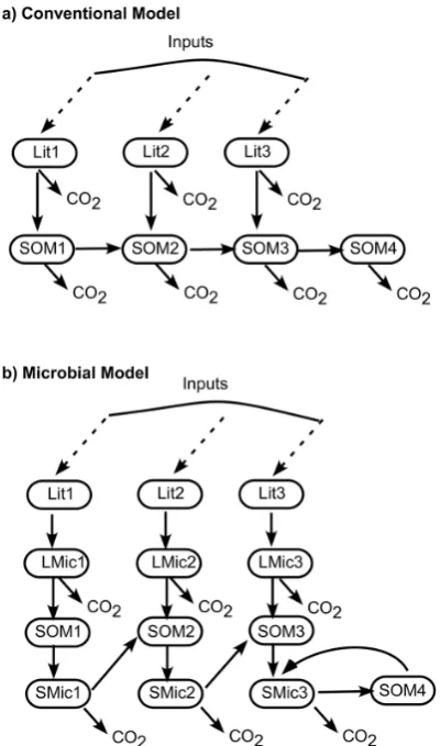
to be included, the source codes have to be significantly mod-ified, including code changes to output new state variables. For example, a recent modeling study has found that incor-porating microbial processes can improve the global soil car-bon projections (Wieder et al., 2013). The modeled processes in that study are compared to the conventional processes in Fig. 1. It can be seen that in order to use this simple new model, ODEs for carbon state variables in litter and soil have to be manually modified and six more ODEs for the microbes have to be added. Users have to manually discern the ODEs and keep track of the state variables, stoichiometries, and their relationship to each process. This is easy when fluxes between different pools only pass through a single microbial population, but in reality the conversion of pools involves microbial consortia. It is tractable when each process only involves at most two state variables as currently represented in CLM, although a significant effort is required to track each variable and process. It becomes a significant burden for the programmers and modelers when complex reaction pathways that involve more variables and processes have to be inte-grated. Users also need to be familiar with the code before they can make efficient updates to it. Maintenance and modi-fication of the current software hierarchy is time consuming, labor intensive, and error prone. These difficulties can be re-solved using the new biogeochemical module presented in this study.

(3)

Fig. 1. Diagram of soil C models. (a) Conventional model and (b) microbial model. Lit, SOM, and Mic stand for C pools for litter,

soil organic, and microbial biomass, respectively. Dashed arrows are plant inputs. Solid arrows are fluxes between pools.

The new biogeochemical module developed in this paper can be readily used to update or incorporate new C, N, P and other nutrient cycle models into CLM and other Earth system models and to evaluate the effects of alternative pro-cess pathways and mechanisms on climate changes. Similar to modeling geochemical reactions using the reaction-based approach that has been commonly used in modeling subsur-face reactive transport (Aguilera et al., 2005; Chilakapati et al., 2000; Yeh et al., 2001), the new biogeochemical mod-ule treats terrestrial C, N, and P cycles as reaction pathways and these pathways are explicitly modeled using the reaction-based approach. The reaction-reaction-based approach requires a self-consistent reaction network, the forming of which with cor-rect stoichiometries is a major challenge not only for mod-eling, but also for process characterization and understand-ing because of the complexity and a large number of biogeo-chemical processes and reactions involved in terrestrial car-bon cycling. To solve this problem from the modeling point of view, a reaction database that can be used to concisely store all biogeochemical reactions in plants, litter, and soil

that can potentially affect carbon cycling processes is devel-oped here. In the following sections, we will first introduce the reaction-based approach, followed by using this approach to develop the generic biogeochemical module in CLM. As a validation, the results from the new module incorporated into CLM were compared with the original CLM-CN. The results were then compared to those using the decomposition model of soil organic matter in CENTURY (Parton et al., 1988) under the CLM modeling framework. A procedure to integrate new processes into the new biogeochemical module is demonstrated using global P cycling as an example (Wang et al., 2010). The model that includes the phosphorus dynam-ics can be used to evaluate the effect of phosphorus on pro-ductivity of terrestrial ecosystems.

2 Methods

2.1 Reaction-based approach

A dynamic reaction system may be defined by reaction path-ways or networks (Yeh et al., 2001). In the reaction-based approach, the mass balance of each state variable of the reac-tion system can be written as

d Ci dt =

N X

k=1

(νik−µik) Rk, (1)

in whichCiis the mass of theith state variable,tis time,Rk is the rate of thekth reaction,vikis the reaction stoichiometry of theith state variable in thekth reaction associated with the products,µikis the reaction stoichiometry of theith state variable in thekth reaction associated with the reactants, and N is the number of reactions. Equation (1) states that the rate of change in the mass of any state variable is due to all reactions that produce or consume that state variable. The whole system can be written in a matrix form as

[I] _dC

dt

=[A]{_R}_. (2) IfMis the total number of state variables in the system, then [I] is anM×Munit matrix,ndC_dtois a vector of length M, and [A] is anM×N matrix, the columnkof which con-sists of stoichiometries of allC_i0s involved in reactionkwith rateRk, which are allowed to vary during the simulation to account for the effects of moisture, temperature, etc. on the reaction stoichiometries.

(4)

Chilakapati et al., 2000). However, many of them depend on third-party commercial software. In this paper, we use a systematic way to derive ODEs and decouple them from fast reactions using matrix row and column operation (ma-trix decomposition) as detailed in Fang et al. (2003). A sim-ple system with one slow reaction and one fast (equilibrium) reaction, and three state variables are used to illustrate the method:

aA↔bB, R1 (R1)

and

A↔cC, R2. (R2)

We define the flux of a substance as a derivative of that substance with respect to time, and it has the dimension of amount of substance per unit volume transformed per unit time. The reaction rate for a single reaction differs from the flux of a substance by the reciprocal of its stoichiometric number in that reaction. The rate of a reaction is always positive, and it can be calculated either as linear or non-linear function. Assuming Reaction (R1) is a slow reaction with reaction rate R1 and Reaction (R2) is a fast adsorp-tion/desorption reaction with reaction rateR2, the simple sys-tem in matrix form can be written as



 1 0 0 0 1 0 0 0 1

     dA dt dB dt dC dt    =  

−a−1

b 0 0 c   R1 R2 . (3)

Equation (3) can be expanded as dA

dt = −aR1−R2, (4)

dB

dt =bR1 (5)

anddC

dt =cR2. (6)

Direct integration of the above ODEs is impractical due to the large rate ofR2, which requires very small time steps. To solve the problem, a direct thermodynamic equilibrium approach, such as a sorption isotherm (Wang et al., 2010), may be employed to model the fast Reaction (R2). The sys-tem can now be solved with two ODEs and one algebraic equation andR2is no longer in any of the ODEs. This can be done by performing column reduction by determining a pivot (nonzero) element in the fast reaction column in matrix [A] of Eq. (2) and using a matrix row operation to convert the column containing the pivot element into a unit column. Element –1 orcin the second column of the reaction matrix in Eq. (3) can be a pivot element. Ifcis chosen as a pivot element, the third row of the matrix equation is first divided bycand then added to the first row to convert the second col-umn of the reaction matrix into a unit colcol-umn. Equation (3) now becomes



 1 0 1_c 0 1 0 0 0 1_c

     dA dt dB dt dC dt    =  

−a0 b 0 0 1   R1 R2 . (7)

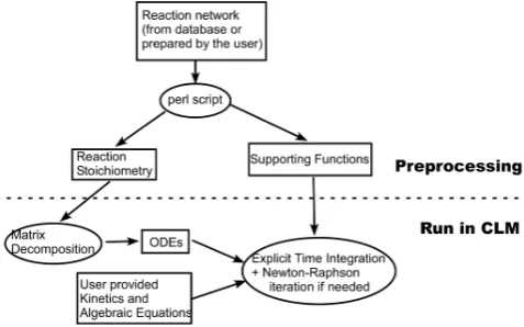
Fig. 2. Diagram of model structure. Rectangles represent model

in-put/output, ovals represent executable programs.

Expanding Eq. (7), we obtain the following: d(A+1/cC)

dt = −aR1, (8)

dB

dt =bR1 (9)

anddC

dt =cR2. (10)

Equation (10) is the only ODE that containsR2and it can be replaced with an algebraic equation (which can be a func-tion of A and C) and solved together with Eqs. (8) and (9). A and C can be solved using Newton–Raphson iteration after (A+1/cC) is solved with explicit time integration.

If the system contains no fast processes, ODEs can be formed by simply expanding the matrix equation provided by the user. Otherwise, column reduction will be performed to generate ODEs containing only slow reactions similar to the procedure above for the simple example. The equations can be solved either using an explicit method or the Newton– Raphson iteration approach. The solver developed in Fang et al. (2003) was modified and is called NGBGC (Next Gener-ation BioGeoChemical Module) hereafter in this study. 2.2 Development of the generic biogeochemical

module

(5)

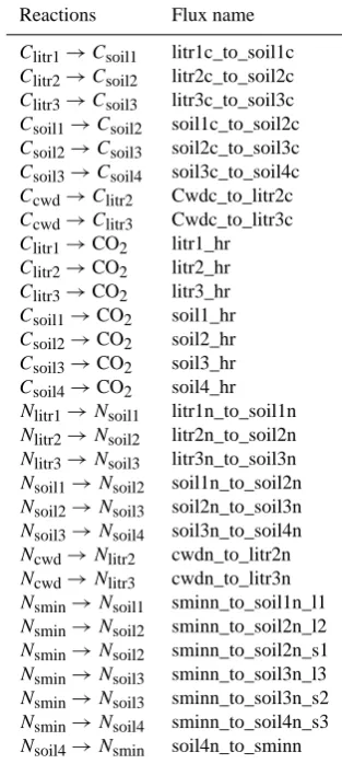
Table 1. Decomposition processes created from the ODEs in

CLM-CN.

Reactions Flux name

Clitr1→Csoil1 litr1c_to_soil1c Clitr2→Csoil2 litr2c_to_soil2c Clitr3→Csoil3 litr3c_to_soil3c Csoil1→Csoil2 soil1c_to_soil2c Csoil2→Csoil3 soil2c_to_soil3c Csoil3→Csoil4 soil3c_to_soil4c Ccwd→Clitr2 Cwdc_to_litr2c Ccwd→Clitr3 Cwdc_to_litr3c Clitr1→CO2 litr1_hr Clitr2→CO2 litr2_hr Clitr3→CO2 litr3_hr Csoil1→CO2 soil1_hr Csoil2→CO2 soil2_hr Csoil3→CO2 soil3_hr Csoil4→CO2 soil4_hr Nlitr1→Nsoil1 litr1n_to_soil1n Nlitr2→Nsoil2 litr2n_to_soil2n Nlitr3→Nsoil3 litr3n_to_soil3n Nsoil1→Nsoil2 soil1n_to_soil2n Nsoil2→Nsoil3 soil2n_to_soil3n Nsoil3→Nsoil4 soil3n_to_soil4n Ncwd→Nlitr2 cwdn_to_litr2n Ncwd→Nlitr3 cwdn_to_litr3n Nsmin→Nsoil1 sminn_to_soil1n_l1 Nsmin→Nsoil2 sminn_to_soil2n_l2 Nsmin→Nsoil2 sminn_to_soil2n_s1 Nsmin→Nsoil3 sminn_to_soil3n_l3 Nsmin→Nsoil3 sminn_to_soil3n_s2 Nsmin→Nsoil4 sminn_to_soil4n_s3 Nsoil4→Nsmin soil4n_to_sminn

functions that later will be compiled with the code in CLM, and the user subroutine in which kinetics or algebraic equa-tions (if any) for each process are defined to generate an exe-cutable. Given a reaction of 2A↔5B, the stoichiometry gen-erated will look like “1−2.0 2 5.0”, i.e., positive number for product, negative number for reactant. The integers “1” and “2” represent substance A and B, respectively. NGBGC will read in the stoichiometries and run matrix decomposition to generate ODEs, which will then be solved using an explicit method. The following illustrates the essence of the proposed generic module and modeling procedures.

To be consistent with the biogeochemical processes com-monly integrated in CLM, such as CLM-CN, we first iden-tified these processes by reversely analyzing the numerical codes that solve the ODEs used in CLM-CN. A reaction net-work was then built based on the identified processes. Table 1 shows the processes involved in the cascade model of litter and soil organic matter decomposition in CN.

In Table 1, C and N are state variables of each pool. The symbol “→” denotes the reaction direction, which is as-sumed to be nonreversible. Variables on the left are reactants

and on the right are products. If a process does not have a re-actant/product, the process represents the source/sink of the state variable. Other variables in the table are defined in the List of Abbreviations in the Appendix (Table A1).

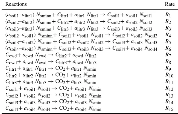
If one were not familiar with the code and processes that the code is written to represent, making changes would be difficult. In a reaction-based approach, by studying the pro-cesses in Table 1 and how the rates were defined in the origi-nal code, we came up with the following decomposition cas-cade processes with balanced elements in Table 2 using the reaction-based approach.

In Table 2, parametera is the N:C ratio for each pool, which is calculated before each new time integration, andC andNare state variables of each pool.R1toR8are decom-position rates, andR9–R15are heterotrophic respiration rates of each pool.

To illustrate the procedure executed in NGBGC, the ODEs for some of the state variables in the form of Eq. (2) using the reactions in Table 2 can be written as follows:

dNlitr1

dt = −alitr1R1−alitr1R9, (11) dNsoil1

dt =asoil1R1 (12)

and dNsmin

dt = −(asoil1−alitr1) R1−(asoil2−alitr2) R2

−(asoil3−alitr3) R3−(asoil2−asoil1) R4−(asoil3−asoil2) R5−(asoil4−asoil3) R6+alitr1R9+alitr2R10+alitr3R11

+asoil1R12+asoil2R13+asoil3R14+asoil4R15. (13) The ODEs for the rest of the state variables based on the reactions in Table 2 can be derived similarly based on the mass balance for each state variable. All the ODEs from the reactions in Table 2 and their reaction kinetics are listed in the Supplement.

The advantages of using such a reaction-based approach are: (1) the meaning of each process is obvious to the users, (2) carbon and nitrogen are explicitly linked in the reaction pathways, and additional variables, such as flux names for N transition in Table 1, are not necessary because they will be handled automatically by NGBGC using the stoichiometries in each process, and (3) new elements can be added to each process in a straightforward way.

If the decomposition model of soil organic matter in CEN-TURY (Parton et al., 1988) is to be used, the pathways with balanced elements are shown in Table 3.

(6)

Table 2. CLM-CN decomposition cascade model.

Reactions Rate

(asoil1–alitr1) Nsminn+Clitr1+alitr1Nlitr1→Csoil1+asoil1Nsoil1 R1

(asoil2–asoil1) Nsminn+Csoil1+asoil1Nsoil1→Csoil2+asoil2Nsoil2 R4

(asoil3–asoil2) Nsminn+Csoil2+asoil2Nsoil2→Csoil3+asoil3Nsoil3 R5

(asoil4–asoil3) Nsminn+Csoil3+asoil3Nsoil3→Csoil4+asoil4Nsoil4 R6 Ccwd+acwdNcwd→Clitr2+acwdNlitr2 R7 Ccwd+acwdNcwd→Clitr3+acwdNlitr3 R8 Clitr1+alitr1Nlitr1→CO2+alitr1Nsmin R9 Clitr2+alitr2Nlitr2→CO2+alitr2Nsmin R10 Clitr3+alitr3Nlitr3→CO2+alitr3Nsmin R11 Csoil1+asoil1Nsoil1→CO2+asoil1Nsmin R12 Csoil2+asoil2Nsoil2→CO2+asoil2Nsmin R13 Csoil3+asoil3Nsoil3→CO2+asoil3Nsmin R14 Csoil4+asoil4Nsoil4→CO2+asoil4Nsmin R15

Table 3. CENTURY decomposition model of soil organic matter.

Reactions Rate

(asoil2–asoil1) Nsmin+Csoil1+asoil1Nsoil1→Csoil2+asoil2Nsoil2 R1

(6 in CLM-CN, 3 for carbon and 3 for nitrogen) used in the original CLM-CN code to solve the ODEs of the state vari-ables into one with a little over 100 lines of code. Unlike the original code, this single subroutine to describe biogeochem-ical processes will not be modified when a new or updated biogeochemical process is to be incorporated, so it can sig-nificantly simplify the programming and more effective ODE solvers for new computational platforms can be introduced easily by modifying a single subroutine.

2.3 Development of process database and script tool

A reaction database is developed so that the reaction network as illustrated in Tables 2 and 3 can be extracted for a specific simulation problem. The database is generic and can be ex-panded when new understandings become available.

Each biogeochemical process in the database has a unique name that is used to track the rate definition in the code and a tag to denote its source so that users have the flexibility to choose those processes either from a particular model (e.g., CLM-CN, CENTURY, etc.) currently used by the modeling community or to introduce new or updated processes. For ex-ample, the microbial model shown in Fig. 1 can be added to the database with the tag “microbial_model”. The entry in the database for carbon flux from the litter pool 1 to the microbial pool 1 in the model can be written as lit1_c(c)↔lmic1_c(c)

!litr1_to_lmic microbial_model, where (c)means the reac-tion is in the soil column of the model grid, litr1_to_lmic is the rate name that will be used in the user subroutine, and microbial_model is the tag. The rate law can be first-order ki-netics, Michaelis–Menten kiki-netics, or any other expressions fitted from the experiment. They are written by the user in the user subroutine.

For users to efficiently update the database, the reactions are grouped into three types: reactions within plants, reac-tions from plants to soil, and reacreac-tions in the soil. The for-mat is provided in the comments of the database so that one can easily update the database with new and updated bio-geochemical processes by only modifying the user subrou-tine for the kinetics of the new processes. A database con-taining those processes reversely identified from CLM-CN can be found in the Supplement. Application of the database is demonstrated in the Results section and the simulation results using the reaction-based approach are benchmarked against those from the existing biogeochemical module, such as CLM-CN.

(7)

each plant functional type (pft):

leafc(p)→litr1c(c), R1, (R3)

leafc(p) →litr2c(c), R2 (R4)

and

leafc(p)→litr3c(c), R3. (R5)

The ODEs for the above three reactions can be written as d[leafc(p)]

dt = −R1−R2−R3, (14)

d[litr1c(c)]

dt =R1, (15)

d[litr2c(c)]

dt =R2 (16)

and d[litr3c(c)]

dt =R3. (17)

In the current version of CLM-CN, the right-hand side of Eq. (14) is represented by a lumped rate:

d[leafc(p)]

dt = −R1−R2−R3= −r (18)

in whichris a function of leafc(p).R1,R2andR3are cal-culated as a fraction ofr based on the fraction of each litter pool in the column and the weight of each pft relative to the column.

Thus, for this type of reaction involving both pft and col-umn state variables, attention needs to be paid when assign-ing reaction rates to the correspondassign-ing ODEs. We have two functions specified in the module: set_column_chem_rate and set_pft_chem_rate; set_pft_chem_rate is called when integrating pft state variables, and set_column_chem_rate is called when integrating column state variables. In the database, a comment is appended for this type of pathway that uses a lumped rate in the ODEs like Eq. (18).

As shown in Fig. 2, a script written in the PERL language is a key component of this generic module. The script has three functions: (1) generate the stoichiometries that are read-able by NGBGC, (2) define and incorporate new processes into CLM, and (3) generate the necessary functions based on a specific reaction network picked from the database. These new functions include pointers that link the reaction names in the database to the defined rate expressions that are used in the code, and state variable names and types (C, N, P, . . . ) identify those reactions (such as those in Table 2) that have dynamic variable stoichiometries, i.e., changing N:C and P:C ratios during the simulation. It also identifies transport properties (mobile or immobile) of each column state vari-able so that a transport capability in CLM such as the one that was recently developed by Tang et al. (2013) (CLM-BeTR) to deal with depth-dependent biogeochemistry in the soil can be used. Note that by identifying the pools that are mobile in

the soil, Eq. (2) can be readily extended to derive the trans-port equations of those pools for the land model (Fang et al., 2003).

The framework developed in this study allows using the same modeling algorithm to simulate C and N cycling in ter-restrial ecosystems with different mathematical representa-tions. For example, microbial models can be evaluated by simply replacing the reaction network formed by conven-tional models with those from the microbial models and new kinetics. The new approach can also readily integrate other nutrient cycles of importance, such as phosphorus (P), potassium (K), and sulfur (S), into the simulation system. Once these processes are in the database, the module gener-ates equations to be solved automatically. But users have the freedom to input user-defined rate expressions with arbitrary form for the new kinetic mechanisms. These expressions are prepared by the user in the user subroutine, which is called by NGBGC during the simulation.

3 Results

3.1 CN model

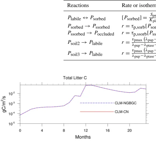
As mentioned in the section above, we have reversely identi-fied those processes used in the CLM-CN model and incor-porated them into our database. All the processes included in CLM-CN were then extracted from the database using the PERL script and input into NGBGC for simulation. All the modeling results presented in this study are defined on a grid with a 1-degree resolution, using the stand-alone CLM with the Qian et al. (2006) atmospheric input data for 2002 and 2003, CO2 level and aerosol deposition for 2000, and arbi-trary initial conditions. Using the new approach and the pro-cesses in Table 1, we were able to obtain identical results as those of the original CLM-CN. We then replaced the decom-position processes with the reactions in Table 2 and refer to our model as CLM-NGBGC. Results of the simulation after two years of integration using the original code and our code were compared and they are exactly the same, as shown in Fig. 3 by the temporal change of total litter C at the Tonzi Ranch site located in the lower foothills of the Sierra Nevada Mountains.

(8)

Table 4. Additional phosphorus dynamics.

Reactions Rate or isotherm Notes

Plabile↔Psorbed [Psorbed] =

Spmax[Plabile]

Kplab+[Plabile] Equilibrium

Psorbed→Pssorbed r=τp,sorb[Psorbed] Kinetic Pssorbed→Poccluded r=τp,ssorb[Pssorbed] Kinetic Psoil2→Plabile r=

vpmax λpup−λptase

λpup−λptase+Kptaseτs,soil2p[Psoil2] Kinetic

Psoil3→Plabile r=

vpmax λpup−λptase

λpup−λptase+Kptaseτs,soil3p[Psoil3] Kinetic

Fig. 3. Comparison of temporal change of total litter C at the Tonzi

Ranch site of the original model (CLM-CN) with our new model (CLM-NGBGC).

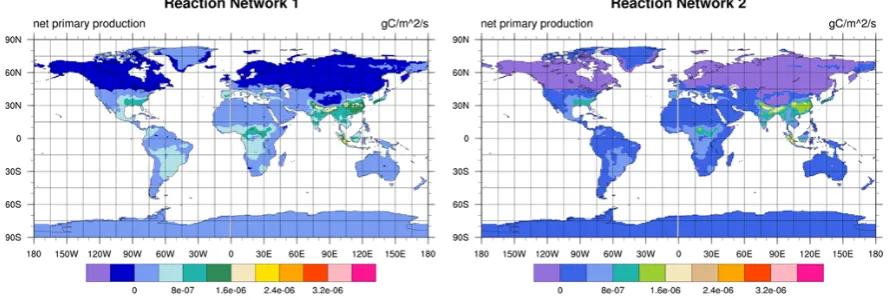
2 hereafter. Spatial distribution of net primary productivity (NPP) and carbon in the soil organic matter soil1 pool after two years of simulation is shown in Figs. 4 and 5, respec-tively. The total NPP calculated using Reaction Network 2 is 89 % of that using Reaction Network 1.

3.2 CNP model

Recent contributions of global mapping of P (Yang et al., 2013) has made it possible to integrate global P cycling into land models. There is no P cycling model in the current CLM framework. To integrate phosphorus cycling into CLM, the allocation of P to live aboveground and belowground and the flow of P in plant litter and different organic soil pools are assumed to follow the allocation of N in CLM-CN: (1) the phenology transition flux of C, N, and P maintains a constant stoichiometry, (2) P is allocated to an additional storage pool after the P needs are satisfied for plant tissues, and (3) the scheme of occurrence of retranslocation of P follows that of N. The stoichiometric relationship of P during decomposi-tion follows that of N in Tables 2 and 3. For instance, R1 in Table 2 is now written as

(bsoil1−blitr1)Plabile+(asoil1−alitr1)Nsmin+Clitr1

+alitr1Nlitr1+blitr1Plitr1

→Csoil1+asoil1Nsoil1+bsoil1Psoil1, (19) wherePlabileis the labile pool of P in the soil and parameter bis the P:C ratio for each pool.

Five extra processes described in Wang et al. (2010) were used to represent the dynamics of labile, sorbed, strongly sorbed, and occluded phosphorus in soil, and biochemical mineralization (breakdown) of slow and passive soil organic P pools through a group of enzymes collectively known as phosphatases (Wang et al., 2007). These processes are shown in Table 4. Sorbed P was assumed to be in equilibrium with labile P, and their relationship is described using the Lang-muir isotherm (Wang et al., 2007).

τp,sorb (0.01) andτp,ssorb (0.01) are rate constants for the sorbed and strongly sorbed P pools in yr−1, respectively. Spmax (50.0) andKplab (64.0) are the maximum amount of sorbed P (g P m−2₎_{and an adsorption constant (g P m}−2_), re-spectively.vpmax(0.1) is the maximum specific biochemical mineralization rate (yr−1)andKptase(150.0) is an empirical constant (gN(gP)−1).λpup(25.0) andλptase(15.0) are the N cost for P uptake and phosphatase production (gN(gP)−1), respectively.

P enters the system through dust deposition and weather-ing and leaves by leachweather-ing. Weatherweather-ing is not soil texture-dependent, but fixed at a constant rate. The dust deposition rate is 0.0017 g P m−2yr−1. The soil P leaching rate is calcu-lated as

r=k[Plabile]. (20)

In this study,kis assumed to be 0.04 yr−1.

The C:P ratios of six plant tissues, leaf, live stem, dead stem, live coarse root, dead coarse root, and fine root, were estimated from Wang et al. as roughly 15 times the C:N ra-tios. The initial C:P ratios for litter and the newly formed soil organic pool are four times their C:N ratios, and the C:P ratios of the other soil organic pools are seven times their C:N ratios.

All parameters for this P cycling model were within the ranges reported in the literature, and were assumed to be con-stant, independent of soil texture or biome in the modeling. Maintenance respiration dependency on P was not consid-ered either. Therefore, this example is for demonstration pur-pose only.

(9)

Fig. 4. NPP distribution using Reaction Network 1 (left) and Reaction Network 2 (right).

Fig. 5. Spatial distribution of C in soil1 pool using Reaction Network 1 (left) and Reaction Network 2 (right).

system, one algebraic equation represented by the Langmuir isotherm is included in the solution process. Using the de-composition approach, the ODE regarding labile P was writ-ten as

d

dt(Plabile+Psorbed)= X

k

(νik−µik)Rk. (21)

These ODEs for P only were then linked with other ODEs involving C and N. After each integration, the combined mass of labile and sorbed P was obtained. The individual mass of labile and sorbed P was solved using Newton iter-ation for the Langmuir equiter-ation. As described before, once the reaction database was updated to include P, and new re-action rate laws such as those in Table 4 were written in a user-defined subroutine of kinetics, the entire set of ODEs was automatically formulated and solved by the NGBGC. If a depth-dependent P were to be considered, only labile P in Eq. (21) would be transported.

Total gross photosynthesis (GPP) for the original CN model was scaled or down-regulated by the N limitation. GPP down-regulation for this CNP model is controlled by the minimum of the N-limiting factor and the P-limiting factor, which are calculated as

xN=min

1, Nsmin FNdemand1t

(22) and

xP=min

1, Plabile FPdemand1t

, (23)

in whichxis the nutrient-limiting factor,Nsminis the amount of mineral N in soil,Plabileis the amount of labile P in the soil, F is the amount of minimal nutrient required to sus-tain a given NPP, and1t is the integration time step of the model. Using the generic approach, this model was imple-mented within a few days and incorporated into the current CLM framework.

With the P weathering rate of 0.05 g P m−2_yr−1_{, almost} no P limiting on productivity was shown. Figures 6 and 7 show the distribution of labile and sorbed P after two years of simulated time. Total labile and sorbed P account for 18 % and 14 % of total P in soil, respectively.

(10)

Fig. 6. Labile P distribution with weathering rate of 0.05 g P m−2yr−1.

Fig. 7. Sorbed P distribution with weathering rate of

0.05 g P m−2yr−1.

is consistent with the simulation in Wang et al. (2010) using this low weathering rate.

As mentioned above, soil texture and biome were not con-sidered in our P model. Maintenance respiration dependency on P was not considered either. Studies have found that the carbon costs of root maintenance respiration in phosphorus-deficient plants could be as high as 39 % of daily photo-synthesis (Meir et al., 2008; Nord et al., 2011; Postma and Lynch, 2011). The model can be improved and applied glob-ally when global P datasets become available.

4 Conclusion

A generic biogeochemistry module was developed that can be used to simulate C, N, and P biogeochemical cycles in the terrestrial biosphere. This new module uses a reaction-based approach in which the overall rate of a state variable is described by summing the rates of all individual processes where this variable is a reactant or product. The approach provides a flexible way to update or add a new process by

Fig. 8. Spatial map of P limitation with weathering rate of

0.01 g P m−2yr−1.

only modifying the kinetic mechanisms for the targeted spe-cific process without the need to modify the integration of specific ODEs as required for the current CLM model. In ad-dition, a database was generated that can store individual bio-geochemical processes used in all ESMs orderly and be read-ily updated when new and updated process models become available. The processes in the database can be efficiently ex-tracted using a PERL script to form a formatted reaction net-work to be used in the generic biogeochemistry module. Bio-geochemical processes represented in different ESMs can be modeled by extracting different pools of reactions from the database. This way, different CN models and biogeochem-ical mechanisms can be compared effectively in the same CLM modeling framework and evaluated using observations by changing the reaction networks and user-defined subrou-tines for kinetics. This framework also allows structural un-certainties related to biogeochemistry models to be assessed with minimal coding efforts.

(11)

Newton–Raphson method to the algebraic equations to solve the steady-state solution. This is especially useful when the decomposition of carbon pools is represented by nonlinear kinetics.

The approach represents a cost-effective way for the CLM community to model biogeochemical processes and provides an efficient way to integrate new and updated process mod-els. In addition, the reaction database approach provides a mutually understandable venue to communicate with biogeo-chemists for improvement of model process representations and even inspire new research.

5 Code availability

The source code of the generic algorithm and PERL script can be obtained upon request. Contact: [email protected]. Appendix A

Table A1. List of abbreviations.

a_cwd N:C (gN g−1C) ratio in coarse woody debris pool

alitr1 N:C (gN g−1C) ratio in litter pool 1

a_litr2 N:C (gN g−1C) ratio in litter pool 2

a_litr3 N:C (gN g−1C) ratio in litter pool 3

asoil1 N:C (gN g−1C) ratio in soil organic matter pool 1

a_soil2 N:C (gN g−1C) ratio in soil organic matter pool 2

a_soil3 N:C (gN g−1C) ratio in soil organic matter pool 3

asoil4 N:C (gN g−1C) ratio in soil organic matter pool 4

b_litr1 P:C (gP g−1C) ratio in litter pool 1

b_soil1 P:C (gP g−1C) ratio in soil organic matter pool 1

C_cwd carbon in coarse woody debris pool

C_litr1 carbon in litter pool 1

Clitr2 carbon in litter pool 2

C_litr3 carbon in litter pool 3

C_soil1 carbon in soil organic matter pool 1

N_cwd nitrogen in coarse woody debris pool

N_litr1 nitrogen in litter pool 1

Nlitr2 nitrogen in litter pool 2

N_litr3 nitrogen in litter pool 3

N_soil1 nitrogen in soil organic matter pool 1

Nsoil4 nitrogen in soil organic matter pool 4

N_smin mineral nitrogen in soil

P_litr1 phosphorus in litter pool 1

Plabile phosphorus in the labile soil pool

P_soil1 phosphorus in soil organic matter pool 1

P_sorbed sorbed phosphorus pool in soil

Pssorbed strongly sorbed phosphorus pool in soil

P_occluded occluded phosphorus pool in soil

Supplementary material related to this article is available online at http://www.geosci-model-dev.net/6/ 1977/2013/gmd-6-1977-2013-supplement.zip.

Acknowledgements. This research has been accomplished through funding support from Pacific Northwest National Laboratory’s Laboratory Directed Research and Development Program. A portion of this research was performed using PNNL Institutional Computing at Pacific Northwest National Laboratory. PNNL is operated by Battelle for the US Department of Energy under Contract DE-AC05-76RL01830.

Edited by: D. Lunt

References

Aguilera, D. R., Jourabchi, P., Spiteri, C., and Regnier, P.: A knowledge-based reactive transport approach for the simulation of biogeochemical dynamics in Earth systems, Geochem. Geo-phys. Geosyst., 6, Q07012, doi:10.1029/2004GC000899, 2005. Allison, S. D. and Martiny, J. B. H.: Resistance, resilience, and

re-dundancy in microbial communities, Proc. Natl. Aca. Sci. USA, 105, 11512–11519, 2008.

Bradford, M. A., Davies, C. A., Frey, S. D., Maddox, T. R., Melillo, J. M., Mohan, J. E., Reynolds, J. F., Treseder, K. K., and Wallenstein, M. D.: Thermal adaptation of soil microbial respirationto elevated temperature, Ecol. Lett., 11, 1316–1327, doi:10.1111/j.1461-0248.2008.01251.x, 2008.

Buendía, C., Kleidon, A., and Porporato, A.: The role of tectonic uplift, climate, and vegetation in the long-term terrestrial phos-phorous cycle, Biogeosciences, 7, 2025–2038, doi:10.5194/bg-7-2025-2010, 2010.

Bünemann, E. K. and Condron, L. M.: Phosphorus and Sulphur cling in Terrestrial Ecosystems, in: Soil Biology, Nutrient Cy-cling in Terrestrial Ecosystems, edited by: Marschner, P. and Rengel Z., Springer, New York, 65–92, 2007.

Chilakapati, A., Yabusaki, S., Szecsody, J., and MacEvoy, W.: Groundwater flow, multicomponent transport and biogeochem-istry: development and application of a coupled process model, J. Contaminant Hydrol., 43, 303–325, 2000.

Fang, Y., Yeh, G. T., and Burgos, W. D.: A general

paradigm to model reaction-based biogeochemical

pro-cesses in batch systems, Water Resour. Res., 39, 1083, doi:10.1029/2002WR001694, 2003.

Goll, D. S., Brovkin, V., Parida, B. R., Reick, C. H., Kattge, J., Re-ich, P. B., van Bodegom, P. M., and Niinemets, Ü.: Nutrient lim-itation reduces land carbon uptake in simulations with a model of combined carbon, nitrogen and phosphorus cycling, Biogeo-sciences, 9, 3547–3569, doi:10.5194/bg-9-3547-2012, 2012. Gu, C., Laverman, A. M., and Pallud, C. E.: Environmental

con-trols on nitrogen and sulfur cycles in surficial aquatic sediments, Front. Microbiol., 3, 45, doi:10.3389/fmicb.2012.00045, 2012. IPCC: Contribution of Working Group I to the Fourth Assessment

(12)

H. L., Cambridge University Press, Cambridge, United Kingdom and New York, NY, USA, 996 pp., 2007.

Lawrence, D. M., Oleson, K. W., Flanner, M. G., Thornton, P. E., Swenson, S. C., Lawrence, P. J., Zeng, X., Yang, Z.-L., Levis, S., Sakaguchi, K., Bonan, G. B., and Slater, A. G.: Parameteri-zation Improvements and Functional and Structural Advances in Version 4 of the Community Land Model, J. Adv. Model. Earth Syst., 3, M03001, doi:10.1029/2011MS000045, 2011.

Luo, Y. Q., Randerson, J. T., Abramowitz, G., Bacour, C., Blyth, E., Carvalhais, N., Ciais, P., Dalmonech, D., Fisher, J. B., Fisher, R., Friedlingstein, P., Hibbard, K., Hoffman, F.,Huntzinger, D., Jones, C. D., Koven, C., Lawrence, D., Li, D. J., Mahecha, M., Niu, S. L., Norby, R., Piao, S. L., Qi, X., Peylin, P., Prentice, I. C., Riley, W., Reichstein, M., Schwalm, C.,Wang, Y. P., Xia, J. Y., Zaehle, S., and Zhou, X. H.: A framework for benchmark-ing landmodels, Biogeosciences, 9, 3857–3874, doi:10.5194/bg-9-3857-2012, 2012.

McGuire, A. D., Melillo, J. M., Kicklighter, D. W., Pan, Y., Xiao, X., Helfrich, J., Moore, B., Vorosmarty, C. J., and Schloss, A. L.: Equilibrium responses of global net primary production and carbon storage to doubled atmospheric carbon dioxide: Sensitiv-ity to changes in vegetation nitrogen concentration, Global Bio-geochem. Cy., 11, 173–189, 1997.

McGuire, K. L. and Treseder, K. K.: Microbial communities and their relevance for ecosystem models: Decomposition as a case study, Soil Biol. Biochem., 42, 529–535, 2010.

Meir, P., Metcalfe, D. B., Costa, A. C. L., and Fisher, R. A.: The fate of assimilated carbon during drought: impacts on respiration in Amazon rainforests, Philos. Trans. Roy. Soc. B-Biol. Sciences, 363, 1849–1855, 2008.

Mitchell, M. J. and Fuller, R. D.: Models of Sulfur Dynamics in For-est and Grassland Ecosystems with Emphasis on Soil Processes, Biogeochem., 5, 133–163, 1988.

Nord, E. A., Shea, K., and Lynch, J. P.: Optimizing reproductive phenology in a two-resource world: a dynamic allocation model of plant growth predicts later reproduction in phosphorus-limited plants, Annals Botany, 108, 391–404, 2011.

Oleson, K. W., Lawrence, D. M., Bonan, G. B. , Flanner, M. G., Kluzek, E., Lawrence, P. J., Levis, S., Swenson, S. C., Thornton, P. E., Dai, A., Decker, M., Dickinson, R., Feddema, J., Heald, C. L., Hoffman, F., Lamarque, J., Mahowald, N., Niu, G., Qian, T., Randerson, J., Running, S., Sakaguchi, K., Slater, A., Stockli, R., Wang, A., Yang, Z., Zeng, X., and Zeng, X.: Technical descrip-tion of version 4.0 of the Community Land Model, NCAR Tech. Note NCAR/TN-478+STR, 257, 2010.

Parton, W. J., Stewart, J. W. B., and Cole, C. V.: Dynamics of C, N, P and S in Grassland Soils – a Model, Biogeochemistry, 5, 109–131, 1988.

Parton, W. J., Holland, E. A., Del Grosso, S. J., Hartman, M. D., Martin, R. E., Mosier, A. R., Ojima, D. S., and Schimel, D. S.: Generalized model for NOx and N2O

emis-sions emisemis-sions from soils, J. Geophys. Res., 106, 17403–17419, doi:10.1029/2001JD900101, 2001.

Postma, J. A. and Lynch, J. P.: Root Cortical Aerenchyma Enhances the Growth of Maize on Soils with Suboptimal Availability of Nitrogen, Phosphorus, and Potassium, Plant Physiol., 156, 1190– 1201, 2011.

Qian, T. T., Dai, A., Trenberth, K. E., and Oleson, K. W.: Simula-tion of global land surface condiSimula-tions from 1948 to 2004, Part I: Forcing data and evaluations, J. Hydrometeorol., 7, 953–975, 2006.

Randerson, J. T., Hoffman, F. M., Thornton, P. E., Mahowald, N. M., Lindsay, K., Lee, Y. H., Nevison, C. D., Doney, S. C., Bo-nan, G., Stockli, R., Covey, C., Running, S. W., and Fung, I. Y.: Systematic assessment of terrestrial biogeochemistry in cou-pled climate-carbon models, Glob. Change Biol., 15, 2462–2484, 2009.

Tang, J. Y., Riley, W. J., Koven, C. D., and Subin, Z. M.: CLM4-BeTR, a generic biogeochemical transport and reaction mod-ule for CLM4: model development, evaluation, and application, Geosci. Model Dev., 6, 127–140, doi:10.5194/gmd-6-127-2013, 2013.

Thornton, P. E. and Rosenbloom, N. A.: Ecosystem model spin-up: Estimating steady state conditions in a coupled terrestrial carbon and nitrogen cycle model, Ecol. Model., 189, 25–48, 2005. Thornton, P. E., Law, B., Gholz, H., Clark, K., Falge, E., Ellsworth,

D., Goldstein, A., Monson, R., Hollinger, D., and Falk, M.: Modeling and measuring the effects of disturbance history and climate on carbon and water budgets in evergreen needleleaf forests, Agr. Forest Meteorol., 113, 185–222, 2002.

Thornton, P. E., Lamarque, J. F., Rosenbloom, N. A., and Mahowald, N. M.: Influence of carbon-nitrogen cycle cou-pling on land model response to CO(2) fertilization and climate variability, Global Biogeochem. Cy., 21, GB4018, doi:10.1029/2006GB002, 2007.

Todd-Brown, K. E. O., Hopkins, F. M., Kivlin, S. N., Talbot, J. M., and Allison, S. D.: A framework for representing microbial de-composition in coupled climate models, Biogeochemistry, 109, 19–33, 2012.

Wang, Y. P., Houlton, B. Z., and Field, C. B.: A model of biogeo-chemical cycles of carbon, nitrogen, and phosphorus including symbiotic nitrogen fixation and phosphatase production, Global Biogeochem. Cy., 21, GB101, doi:10.1029/2006GB002797, 2007.

Wang, Y. P., Law, R. M., and Pak, B.: A global model of carbon, nitrogen and phosphorus cycles for the terrestrial biosphere, Bio-geosciences, 7, 2261–2282, doi:10.5194/bg-7-2261-2010, 2010. Wieder, W. R., Bonan, G. B., and Allison, S. D.: Global soil carbon projections are improved by modelling mi-crobial processes, Nature Climate Change, 3, 909–912, doi:10.1038/NCLIMATE1951, 2013.

Yang, X., Post, W. M., Thornton, P. E., and Jain, A.: The distri-bution of soil phosphorus for global biogeochemical modeling, Biogeosciences, 10, 2525–2537, doi:10.5194/bg-10-2525-2013, 2013.