Parallel algorithms for planar and spherical Delaunay construction with an application to centroidal Voronoi tessellations

(1)

Geosci. Model Dev., 6, 1353–1365, 2013 www.geosci-model-dev.net/6/1353/2013/ doi:10.5194/gmd-6-1353-2013

EGU Journal Logos (RGB)

Advances in

Geosciences

Open Access

Natural Hazards

and Earth System

Sciences

Open Access

Annales

Geophysicae

Open Access

Nonlinear Processes

in Geophysics

Open Access

Atmospheric

Chemistry

and Physics

Open Access

Atmospheric

Chemistry

and Physics

Open Access

Discussions

Atmospheric

Measurement

Techniques

Open Access

Atmospheric

Measurement

Techniques

Open Access

Discussions

Biogeosciences

Open Access Open Access

Biogeosciences

Discussions

Climate

of the Past

Climate

of the Past

Discussions

Earth System

Dynamics

Earth System

Dynamics

Discussions

Geoscientific

Instrumentation

Methods and

Data Systems

Open Access

_{Geoscientific}

Instrumentation

Methods and

Data Systems

Open Access

Discussions

Geoscientific

Model Development

Geoscientific

Model Development

Discussions

Hydrology and

Earth System

Sciences

Open Access

Hydrology and

Earth System

Sciences

Open Access

Discussions

Ocean Science

Discussions

Solid Earth

Discussions

The Cryosphere

Discussions

Natural Hazards

and Earth System

Sciences

Open Access

Discussions

Parallel algorithms for planar and spherical Delaunay construction

with an application to centroidal Voronoi tessellations

D. W. Jacobsen1,2, M. Gunzburger1, T. Ringler2, J. Burkardt1, and J. Peterson1

1_{Department of Scientific Computing, Florida State University, Tallahassee, FL 32306, USA} 2_{Theoretical Division, Los Alamos National Laboratory, Los Alamos, NM 87545, USA}

Correspondence to: D. W. Jacobsen ([email protected])

Received: 5 February 2013 – Published in Geosci. Model Dev. Discuss.: 22 February 2013 Revised: 18 June 2013 – Accepted: 2 July 2013 – Published: 30 August 2013

Abstract. A new algorithm, featuring overlapping domain

decompositions, for the parallel construction of Delaunay and Voronoi tessellations is developed. Overlapping allows for the seamless stitching of the partial pieces of the global Delaunay tessellations constructed by individual processors. The algorithm is then modified, by the addition of stereo-graphic projections, to handle the parallel construction of spherical Delaunay and Voronoi tessellations. The algo-rithms are then embedded into algoalgo-rithms for the paral-lel construction of planar and spherical centroidal Voronoi tessellations that require multiple constructions of Delau-nay tessellations. This combination of overlapping domain decompositions with stereographic projections provides a unique algorithm for the construction of spherical meshes that can be used in climate simulations. Computational tests are used to demonstrate the efficiency and scalability of the algorithms for spherical Delaunay and centroidal Voronoi tessellations. Compared to serial versions of the algorithm and to STRIPACK-based approaches, the new parallel algo-rithm results in speedups for the construction of spherical centroidal Voronoi tessellations and spherical Delaunay tri-angulations.

1 Introduction

Voronoi diagrams and their dual Delaunay tessellations have become, in many settings, natural choices for spatial grid-ing due to their ability to handle arbitrary boundaries and refinement well. Such grids are used in a wide range of ap-plications and can, in principle, be created for almost any geometry in two and higher dimensions. The recent trend towards the exascale in most aspects of high-performance

computing further demands fast algorithms for the genera-tion of high-resolugenera-tion spatial meshes that are also of high quality, e.g. featuring variable resolution with smooth tran-sition regions; otherwise, the meshing part can dominate the rest of the discretization and solution processes. However, creating such meshes can be time consuming, especially for high-quality, high-resolution meshing. Attempts to speed up the generation of Delaunay tessellations via parallel divide-and-conquer algorithms were made in, e.g. Cignoni et al. (1998); Chernikov and Chrisochoides (2008), however these approaches are restricted to two-dimensional planar surfaces. With the current need for high, variable-resolution grid gen-erators in mind, we first develop a new algorithm that makes use of a novel approach to domain decomposition for the fast, parallel generation of Delaunay and Voronoi grids in Euclidean domains.

Centroidal Voronoi tessellations provide one approach for high-quality Delaunay and Voronoi grid generation (Du et al., 1999, 2003b, 2006b; Du and Gunzburger, 2002; Nguyen et al., 2008). The efficient construction of such grids involves an iterative process (Du et al., 1999) that calls for the determination of multiple Delaunay tessellations; we show how our new parallel Delaunay algorithm is especially use-ful in this context.

(2)

1354 D. W. Jacobsen et al.: Parallel algorithms for Delaunay construction

(2008), to transform these tasks into planar Delaunay con-structions for which we apply the new parallel algorithm we have developed for that purpose. Spherical centroidal Voronoi tessellation (SCVT) based grids are especially de-sirable in climate modelling because they not only provide for precise grid refinement, but also feature smooth transi-tion regions (Ringler et al., 2011, 2013). We show how such grids can be generated using the new parallel algorithm for spherical Delaunay tessellations.

The paper is organized in the following fashion. In Sect. 2.1, we present our new parallel algorithm for the con-struction of such tessellations. In Sect. 2.2, we provide a brief discussion of centroidal Voronoi tessellations (CVTs) fol-lowed by showing how the new parallel Delaunay tessella-tion algorithm can be incorporated into an efficient method for the construction of CVTs. In Sect. 3.1, we provide a short review of stereographic projections followed, in Sect. 3.2, by a presentation of the new parallel algorithm for the con-struction of spherical Delaunay and Voronoi tessellations. In Sect. 3.3, we consider the parallel construction of spherical CVTs. In Sect. 4, the results of numerical experiments and demonstrations of the new algorithms are given; for the sake of brevity, we only consider the algorithms for grid genera-tion on the sphere. Finally, in Sect. 5, concluding remarks are provided.

2 Parallel Delaunay and Voronoi tessellation construction in_Rk

In this section, we present a new method for the construction of Delaunay and Voronoi tessellations. The algorithms are first presented in_R2and later extended to_R3.

2.1 Parallel algorithm for Delaunay tessellation construction

The construction of planar Delaunay triangulations in paral-lel has been of interest for several years; see, e.g. Amato and Preparata (1993); Cignoni et al. (1998); Zhou et al. (2001); Batista et al. (2010). Typically, such algorithms divide the point set up into several smaller subsets, each of which can then be triangulated independently from the others. The re-sulting triangulations need to be stitched together to form a global triangulation. This stitching, or merge step, is typi-cally computed serially because one may need to modify sig-nificant portions of the individual triangulations. The merge step is the main difference between the different parallel al-gorithms. Here, we provide a new alternative merge step that, because no modifications of the individual triangulations are needed, can be performed in parallel.

We are given a set of points P = {xj}n_j=1 in a given

domain ⊂_Rk. We begin by covering by a set S= {Sk(ck, rk)}Nk=1ofNoverlapping spheresSk, each of which is

defined by a centre pointckand radiusrk. For each sphereSk,

a connectivity or neighbour list is defined which consists of the indices of all the spheresSi∈S,i6=k, that overlap with

Sk. From the given point set P, we then create N smaller point sets Pk, k=1, . . . , N, each of which consists of the

points inP which are in the sphereSk. Due to the overlap

of the spheresSk, a point inP may belong to multiple points

setsPk. This defines what we are referring to as our sorting

method. The presented sort method is the simplest to under-stand, but provides issues with load balancing on variable resolution meshes. For that reason, we use an alternate sort method in practice which is described Sect. 2.1.1.

The next step is to construct theN Delaunay tessellations

Tk,k=1, . . . , N, of theN point sets Pk,k=1, . . . , N. For this purpose, one can use any Delaunay tessellation method at one’s disposal; for example, in the plane, one can use the Delaunay triangulator that is part of the Triangle software of Shewchuk (1996). A note should be made, that these triangu-lation software packages only aid in the computation of the triangulation. For example, they can not be used to determine which points should be triangulated. These Delaunay tessel-lations, of course, can be constructed completely in parallel after assigning one point setPkto each ofNprocessors.

At this point, we are almost but not quite ready to merge theN local Delaunay tessellations into a single global one. Before doing so, we deal with the fact that although, by con-struction, the tessellationTkof the point setPkis a Delaunay

tessellation ofPk, there are very likely to be simplices in the

tessellation Tk that may not be globally Delaunay, i.e. that may not be Delaunay with respect to points inP that are not inPk. This follows because the points in anyTk are un-aware of the triangles and points outside ofSk so that there may be points inP that are not inPk that lie within the cir-cumsphere of a simplex inTk. In fact, only simplices whose circumspheres are completely contained inside of the ballSk

are guaranteed to be globally Delaunay; those points satisfy the criteria

||ck−bci|| +bri < rk, (1)

where_bciandbri are the centre and radius of the circumsphere

of thei-th triangle in the local Delaunay tessellationTk.

So, at this point, for eachk=1, . . . , N, we construct the triangulationbTk by discarding all simplices in the local

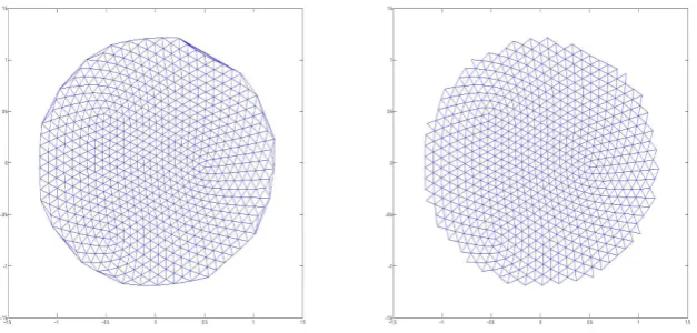
De-launay tessellation Tk whose circumspheres are not com-pletely contained inSk, i.e. all simplices that do not satisfy Eq. (1). Figure 1 shows one of the local Delaunay triangula-tionsTk and the triangulationTkb after the deletion of

trian-gles that are not guaranteed to satisfy the Delaunay property globally.

The final step is to merge theNmodified tessellationsTbk, k=1, . . . , N, that have been constructed completely in paral-lel into a single global tessellation. The key observation here is that each regional tessellationTbk is now exactly a

por-tion of the global Delaunay tessellapor-tion because if two lo-cal tessellationsTbi andTbkoverlap, they must coincide

(3)

D. W. Jacobsen et al.: Parallel algorithms for Delaunay construction 1355 points inPthat are not inPk. This follows because the points in anyTkare unaware of the triangles

and points outside ofSkso that there may be points inPthat are not inPkthat lie within the

circum-sphere of a simplex inTk. In fact, only simplices whose circumspheres are completely contained

inside of the ballSkare guaranteed to be globally Delaunay; those points satisfy the criteria

||ck−bci||+bri< rk, (1)

wherebciandbriare the centre and radius of the circumsphere of theith triangle in the local Delaunay

tessellationTk.

So, at this point, for eachk= 1,...,N, we construct the triangulationTbk by discarding all

sim-plices in the local Delaunay tessellationTkwhose circumspheres are not completely contained inSk,

i.e., all simplices that do not satisfy (1). Figure 1 shows one of the local Delaunay triangulationsTk

120

and the triangulationTbkafter the deletion of triangles that are not guaranteed to satisfy the Delaunay

property globally.

Fig. 1. A local Delaunay triangulationTk(left) and the triangulationTbkafter the deletion of triangles that are

not guaranteed to satisfy the Delaunay property globally.

The final step is to merge the N modified tessellations Tbk,k= 1,...,N, that have been

con-structed completely in parallel into a single global tessellation. The key observation here is that

each regional tessellationTbkis now exactly a portion of the global Delaunay tessellation because if

125

two local tessellationsTbiandTbk overlap, they must coincide wherever they overlap. This follows

from the uniqueness property of the Delaunay tessellations. Thus, the union of the local Delaunay

tessellations is the global Delaunay tessellation; by using an overlapping domain decomposition,

the stitching of the regional Delaunay tessellations into a global one is transparent. Of course, some bookkeeping chores have to be done such as rewriting simplex information in terms of global point 130

indices and counting overlapping simplices only once.

A final note is that the radii{rk}Nk=1 should be chosen large enough so that there are no gaps

5

Fig. 1. A local Delaunay triangulationTk (left) and the triangulationbT_kafter the deletion of triangles that are not guaranteed to satisfy the

Delaunay property globally.

of the Delaunay tessellations. Thus, the union of the local Delaunay tessellations is the global Delaunay tessellation; by using an overlapping domain decomposition, the stitch-ing of the regional Delaunay tessellations into a global one is transparent. Of course, some bookkeeping chores have to be done such as rewriting simplex information in terms of global point indices and counting overlapping simplices only once.

In summary, the algorithm for the construction of a Delau-nay tessellation in parallel consists of the following steps:

– define overlapping ballsSk,k=1, . . . , N, that cover the

given region;

– sort the given point set P into the subsets Pk, k= 1, . . . , N, each containing points inP that are inSk;

– fork=1, . . . , N, construct in parallel theN Delaunay tessellationsTk of the points setsPk;

– fork=1, . . . , N, construct in parallel the tessellationbTk

by removing fromTk all simplices that are not guaran-teed to satisfy the circumsphere property;

– construct the Delaunay tessellation ofP as the union of theNmodified Delaunay tessellations{Tbk}N_k=1.

Once a Delaunay tessellation is determined, it is an easy mat-ter, at least for domains inR2andR3, to construct the dual

Voronoi tessellation; see, e.g. Okabe et al. (2000).

2.1.1 Methods for decomposing global point set

In Sect. 2.1, an initial method was presented for distribut-ing points between regions. We refer to this method as a dis-tance sort. The disdis-tance between a point and a region centre is computed, and if the distance is less than the region’s ra-dius the point is considered for triangulation. The key diffi-culty for this sort method is determining a radius which pro-vides enough overlap, without including significantly more

points than are required. This is an even greater challenge when considering variable resolution meshes and regions that straddle both fine and coarse regions.

In order to properly sort the points, the overlap of the re-gions need to be large enough to satisfy the following three requirements:

– all points contained in a region’s Voronoi cell are not

vertices of any non-Delaunay triangles;

– the resulting triangulation includes all Delaunay

trian-gles for which owned points are vertices of;

– the point set defines all triangles whose circumcircles

fall in the region’s Voronoi cell.

If all three of these are satisfied, the point set can be used in any of the algorithms described in this paper.

Whereas we have yet to describe a method for the choice of region radius, let us first begin by describing the two ex-tremes. First, consider a radius that encompasses the entire domain. This obviously provides enough overlap to guaran-tee the three conditions are satisfied. Second, consider a ra-dius that is equivalent to the edges of the region’s Voronoi cell, and no larger. In this case, the overlap is obviously in-sufficient to satisfy the three conditions. This can be seen if we assume at least one non-Delaunay triangle exists at the boundary of the Voronoi cell, in which case both criteria 1 and 2 are not met.

In practice, choosing the radii{rk}N

k=1 to be equal to the

maximum distance from the centreck of its ball Sk to the

centre of all its adjacent balls allows enough overlap in quasi-uniform cases. However, this method still fails to provide enough overlap in certain cases. All of the failures occur when the global point set does not include enough points for the decomposition of choice. Before discussing the target number of points for a given decomposition, an alternative sorting method is introduced.

(4)

alternative sorting method. We refer to this sorting method as the Voronoi sort. In this case, the method for sorting points makes use of the Voronoi property that all points contained within a Voronoi cell are closer to that cell’s generator than any other generator in the set. It is important to note that the coarse Voronoi cells used for domain decomposition here are not the same as Voronoi cells related to the Delaunay triangulation we are attempting to construct. To begin, the point set is divided into the Voronoi cells defined by the re-gion’s centre, and its neighbour’s region centres. The union of the owned region’s point set and its immediately adjacent region’s point sets defines the final set of points for triangu-lation.

As with the distance sort, the Voronoi sort meets all of the criteria for use in the described algorithms. However, it can also still fail in certain cases. Both sort methods can fail if the target point set is too small for the target decomposition. In this case, one or more regions do not include enough points to correctly compute a triangulation through any method. In practice, these algorithms fail if the decomposition includes more than two regionsN, and the point set contains less than 16N points, or two bisections. For example, a 12 processor decomposition cannot be used with a target of 42 points, but a 12 processor decomposition can be used with a target of 162 points.

In general, the decomposition should be created using the target density function to provide optimal load balancing, and to improve robustness of the algorithm. Results for these sort methods are presented in Sect. 4.2.2.

2.2 Application to the construction of centroidal Voronoi and Delaunay tessellations

Given a Voronoi tessellationV = {Vj}nj=1of a bounded

re-gion ⊂_Rk corresponding to the set of generators P= {xj}n_j=1and given a nonnegative functionρ(x)defined over , referred to as the point-density function, we can define the centre of mass or centroidx∗

jof each Voronoi region as

x∗_j=

R

Vjxρ(x)dx

R

Vjρ(x)dx

, j =1, . . . , n. (2)

In general,xj6=x∗_j, i.e. the generators of the Voronoi cells

do not coincide with the centres of mass of those cells. The special case for whichxj=x∗_j for all j=1, . . . , n, i.e. for

which all the generators coincide with the centres of mass of their Voronoi regions, is referred to as a centroidal Voronoi tessellation (CVT).

Given,n, andρ(x), a CVT ofmust be constructed. The simplest means for doing so is Lloyd’s method (Lloyd, 1982) in which, starting with an initial set ofndistinct gener-ators, one constructs the corresponding Voronoi tessellation, then determines the centroid of each of the Voronoi cells, and then moves each generator to the centroid of its Voronoi cell. These steps are repeated until satisfactory convergence

is achieved, e.g. until the movement of generators falls be-low a prescribed tolerance. The convergence properties of Lloyd’s method are rigorously studied in Du et al. (2006a).

The point-density functionρ plays a crucial role in how the converged generators are distributed and the relative sizes of the corresponding Voronoi cells. If we arbitrarily select two Voronoi cellsVi andVj from a CVT, their grid spacing

and density are related as

hi

hj ≈

_ρ(_x

j)

ρ(xi)

_d₊₂1

, (3)

wherehidenotes a measure of the linear dimension, e.g. the diameter, of the cellVi andxi denotes a point, e.g. the

gen-erator, in Vi. Thus, the point-density function can be used to produce nonuniform grids in either a passive or adaptive manner by prescribing aρor by connectingρto an error in-dicator, respectively. Although the relation Eq. (3) is at the present time a conjecture, its validity has been demonstrated through many numerical studies; see, e.g. Du et al. (1999); Ringler et al. (2011). CVTs and their dual Delaunay tes-sellations have been successfully used for the generation of high-quality nonuniform grids; see, e.g. Du and Gunzburger (2002); Du et al. (2003b, 2006b); Ju et al. (2011); Nguyen et al. (2008).

As defined above, every iteration of Lloyd’s method re-quires the construction of the Voronoi tessellation of the cur-rent set of generators followed by the determination of the centroids of the Voronoi cells. However, the construction of the Voronoi tessellation can be avoided until after the iter-ation has converged and instead, the iterative process can be carried out with only Delaunay tessellation constructions. Thus, the first task within every iteration of Lloyd’s method is to construct the Delaunay tessellation of the current set of generators. The parallel algorithm for the generation of De-launay tessellations given in Sect. 2.1 is thus especially use-ful in reducing the costs of the multiple tessellations needed in CVT construction.

(5)

D. W. Jacobsen et al.: Parallel algorithms for Delaunay construction 1357

determine the centroids of the Voronoi cells. Thus, because both steps within each Lloyd iteration can be performed us-ing only the Delaunay triangulation, determinus-ing the gener-ators of a CVT does not require construction of any Voronoi tessellations nor does it require any mesh connectivity infor-mation. If one is interested in the CVT, one need only con-struct a single Voronoi tessellation after the Lloyd iteration has converged; if one is interested in the Delaunay tessella-tion corresponding to the CVT, then no Voronoi constructessella-tion is needed.

To make this algorithm parallel, one can compute the Voronoi cell centroids using the local Delaunay tessellations and not on the stitched-together global one. However, be-cause the local Delaunay tessellations overlap, one has to en-sure that each generator is only updated by one region, i.e. by only one processor. This can be done using one of a variety of domain decomposition methods. We use a coarse Voronoi diagram corresponding to the region centresck. Each

proces-sor only updates the generators that are inside of its coarse Voronoi cell. Because Voronoi cells are non-overlapping, each generator will only get updated by one processor. Af-ter all the generators are updated, each coarse region needs to transfer its newly updated points only to its adjacent re-gions and not to all active processors. This limits each pro-cessor’s communications to roughly six sends and receives, regardless of the total number of processors used.

We use two metrics to check for the convergence of the Lloyd iteration, namely the`2 and`∞ norms of generator

movement given by

`2norm=

1

n n

X

j=1

(xold_j −xnew_j )21/2 and

`∞norm= max

j=1,...,n(

|xold_j −xnew_j |),

respectively, are compared with a given tolerance; here, old and new refer to the previous and current Lloyd iterates. If either norm falls below the tolerance, the iterative process is deemed to have converged. The`∞norm is more strict, but

both norms follow similar convergence paths when plotted against the iteration number.

A variety of point sets can be used to initiate Lloyd’s method for CVT construction. The obvious one is Monte Carlo points (Metropolis and Ulam, 1949). These can either be sampled uniformly overor sampled according to the point-density functionρ(x). The latter approach usually re-duces the number of iterations required for convergence. One can instead use a bisection method to build fine grids from a coarse grid (Heikes and Randall, 1995). To create a bisec-tion grid, a coarse CVT is constructed using as few points as possible. After this coarse grid is converged, inR2, one

would add the midpoint of every Voronoi cell edge or Delau-nay triangle edge to the set of points. This causes the overall grid spacing to be reduced by roughly a factor of two in every cell so that the refined point set is roughly four times larger.

In summary, the algorithm for the construction of a CVT in parallel consists of the following steps; the steps in Roman font are the same as in the algorithm of Sect. 2.1 whereas the italicized steps, as well as the do loop, are additions for CVT construction:

– define overlapping balls that cover the given region;

– while not converged do

– sort the current point set;

– construct in parallel the local Delaunay

tessella-tions;

– remove from the Delaunay tessellations simplices

which are not guaranteed to satisfy the circum-sphere property;

– in parallel, determine the centroids of the Voronoi

cells by integrating over simplices;

– move each generator to the corresponding cell

cen-troid;

– test the convergence criteria;

– communicate new generator positions to

neigh-bouring balls;

– end

– construct the Delaunay tessellation corresponding to the

CVT as the union of the modified local Delaunay tessel-lations.

3 Parallel Delaunay and Voronoi tessellation construction on the sphere

Replacing the planar constructs of Delaunay triangulations and Voronoi tessellations with their analogous components on the sphere, i.e. on the surface of a ball inR3, creates the

(6)

3.1 Stereographic projections

Stereographic projections are special mappings between the surface of a sphere and a plane tangent to the sphere. Not only are stereographic projections conformal mappings, meaning that angles are preserved, but they also preserve circularity, meaning that circles on the sphere are mapped to circles on the plane. Stereographic projections also map the interior of these circles to the interior of the mapped circles (Bowers et al., 1998; Saalfeld, 1999). For our purposes, the impor-tance of circularity preservation is that it implies that stereo-graphic projections preserve the Delaunay circumcircle prop-erty. This follows because triangle circumcircles (along with their interiors) are preserved. Therefore, Delaunay triangu-lations on the sphere are mapped to Delaunay triangutriangu-lations on the plane and conversely. As a result, stereographic pro-jections can be used to construct a Delaunay triangulation of a portion of the sphere by first constructing a Delaunay tri-angulation in the plane, which is a simpler and well-studied task.

Without loss of generality, we assume that we are given the unit sphere inR3centred at the origin. We are also given

a plane tangent to the sphere at the pointt. The focus pointf

is defined as the reflection oftabout the centre of the sphere, i.e.f is the antipode oft. Letpdenote a point on the unit sphere. The stereographic projection ofponto the plane tan-gent attis the pointqon the plane defined by

q=sp+(1−s)f, where s=2 1

f·(f−p). (4)

For our purposes, it is more convenient to define the projec-tion relative tot rather than f. The simple substitution of

f= −tinto Eq. (4) results in

q=sp+(s−1)t, where s=2 1

t·(p+t). (5)

The definitions Eqs. (4) and (5) can also be used to define stereographic projections in_Rk_for_{k >}_3.

3.2 Parallel algorithm for spherical Delaunay triangulation construction

A spherical Delaunay triangulation (SDT) is the Delaunay triangulation of a point setP defined on the surface of the sphere. We adapt the algorithm developed in Sect. 2.1 for domains in_Rk _{to develop a parallel algorithm for the}

con-struction of SDTs. The most important adaptation is to use stereographic projections so that the actual construction of Delaunay triangulations is done on planar domains.

We are now given a set of pointsP = {xj}n_j=1on a subset of the sphere;may be the whole sphere. We begin by coveringby a setU= {Uk(tk, rk)}N_k=1 ofN overlapping

“umbrellas” or spherical capsUk, each of which is defined

by a centre pointtk and geodesic radiusrk. See Fig. 2a. For

each spherical capUk, a connectivity (or neighbours) list is

(a)

develop a parallel algorithm for the construction of SDTs. The most important adaptation is to use

stereographic projections so that the actual construction of Delaunay triangulations is done on planar

domains.

We are now given a set of points

P

=

{

x

_j

}

n

j=1

on a subset

Ω

of the sphere;

Ω

may be the whole

260

sphere. We begin by covering

Ω

by a set

U

=

{

U

k

(

t

k

,r

k

)

}

Nk=1

of

N

overlapping “umbrellas” or

spherical caps

U

k

, each of which is defined by a centre point

t

k

and geodesic radius

r

k

. See the left

plot in Fig. 4. For each spherical cap

U

k

, a connectivity (or neighbours) list is defined that consists

of the indices of all the spherical caps

U

i

∈

U

,

i

6 =

k

, that overlap with

U

k

. From the given point set

P

, we then create

N

smaller point sets

P

k

,

k

= 1

,...,N

, each of which consists of the points in

P

265

which are in the spherical cap

U

k

. Due to the overlap of the spherical caps

U

k

, a point in

P

may end

up belonging to multiple points sets

P

k

.

Fig. 4. Left: An overlapping subdivision of the sphere into N= 12spherical caps. The cap centrestk are

the projections onto the sphere of the centroids of the 12 pentagons of the inscribed regular icosahedron. Each

coloured ring represents the edge of cap of radiusrk. Right: A 10,242 generator Delaunay triangulation by the

parallel algorithm

At this point in Sect. 2.2, we assigned each of the point subsets

P

k

to a processor and constructed

N

Delaunay tessellations in parallel. Before doing so in the spherical case, we project each of the

point sets

P

k

onto the plane tangent at the corresponding point

t

k

. This additional step allows each

270

processor to construct a planar Delaunay triangulation instead of spherical one. Specifically, for

each

k

, we construct the planar point set

P

e

k

=

S

(

P

k

;

t

k

)

, where

S

(

P

k

;

t

k

)

denotes the stereographic

projection of the points in

P

k

onto the plane tangent to the sphere at the point

t

k

. We then assign each

of the point sets

P

e

k

to a different processor and have each processor construct the planar Delaunay

triangulation of its point set

P

e

k

. Because stereographic projections preserve circularity and therefore

275

preserve the Delaunay circumcircle property, it is then just a simple matter of keeping track of

triangle vertex and edge indices to define the spherical Delaunay triangulations of the point sets

P

k

.

As in Sect. 2.2, we now proceed to remove spherical triangles that are not guaranteed to be

Delaunay with respect to the global point set

P

. Instead of (1), in the spherical case, triangles must

11

(b)

develop a parallel algorithm for the construction of SDTs. The most important adaptation is to use

stereographic projections so that the actual construction of Delaunay triangulations is done on planar

domains.

We are now given a set of pointsP={xj}nj=1on a subsetΩof the sphere;Ωmay be the whole

260

sphere. We begin by covering Ωby a set U={Uk(tk,rk)}Nk=1 ofN overlapping “umbrellas” or

spherical capsUk, each of which is defined by a centre pointtkand geodesic radiusrk. See the left

plot in Fig. 4. For each spherical capUk, a connectivity (or neighbours) list is defined that consists

of the indices of all the spherical capsUi∈U,i6=k, that overlap withUk. From the given point set

P, we then createN smaller point setsPk,k= 1,...,N, each of which consists of the points inP 265

which are in the spherical capUk. Due to the overlap of the spherical capsUk, a point inP may end

up belonging to multiple points setsPk.

Fig. 4. Left: An overlapping subdivision of the sphere intoN= 12spherical caps. The cap centres tk are the projections onto the sphere of the centroids of the 12 pentagons of the inscribed regular icosahedron. Each coloured ring represents the edge of cap of radiusrk. Right: A 10,242 generator Delaunay triangulation by the parallel algorithm

At this point in Sect. 2.2, we assigned each of the point subsetsPkto a processor and constructed

N Delaunay tessellations in parallel. Before doing so in the spherical case, we project each of the

point setsPkonto the plane tangent at the corresponding pointtk. This additional step allows each 270

processor to construct a planar Delaunay triangulation instead of spherical one. Specifically, for

eachk, we construct the planar point setPek=S(Pk;tk), whereS(Pk;tk)denotes the stereographic

projection of the points inPkonto the plane tangent to the sphere at the pointtk. We then assign each

of the point setsPekto a different processor and have each processor construct the planar Delaunay

triangulation of its point setPek. Because stereographic projections preserve circularity and therefore 275

preserve the Delaunay circumcircle property, it is then just a simple matter of keeping track of

triangle vertex and edge indices to define the spherical Delaunay triangulations of the point setsPk.

As in Sect. 2.2, we now proceed to remove spherical triangles that are not guaranteed to be

Delaunay with respect to the global point setP. Instead of (1), in the spherical case, triangles must

11

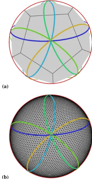
Fig. 2. (a) An overlapping subdivision of the sphere intoN=12 spherical caps. The cap centres tk are the projections onto the

sphere of the centroids of the 12 pentagons of the inscribed reg-ular icosahedron. Each coloured ring represents the edge of cap of radiusrk. (b) A 10 242 generator Delaunay triangulation by the

par-allel algorithm.

defined that consists of the indices of all the spherical caps

Ui∈U,i6=k, that overlap withUk. From the given point set P, we then createNsmaller point setsPk,k=1, . . . , N, each

of which consists of the points inP which are in the spherical capUk. Due to the overlap of the spherical capsUk, a point

inP may end up belonging to multiple points setsPk.

At this point in Sect. 2.1, we assigned each of the point subsets Pk to a processor and constructed N Delaunay

tessellations in parallel. Before doing so in the spherical case, we project each of the point setsPk onto the plane tangent at the corresponding point tk. This additional step allows

each processor to construct a planar Delaunay triangulation instead of spherical one. Specifically, for each k, we con-struct the planar point setPek=S(Pk;tk), whereS(Pk;tk)

denotes the stereographic projection of the points inPk onto

the plane tangent to the sphere at the pointtk. We then

as-sign each of the point setsPek to a different processor and

have each processor construct the planar Delaunay triangu-lation of its point setPek. Because stereographic projections

(7)

track of triangle vertex and edge indices to define the spheri-cal Delaunay triangulations of the point setsPk.

As in Sect. 2.1, we now proceed to remove spherical tri-angles that are not guaranteed to be Delaunay with respect to the global point setP. Instead of Eq. (1), in the spherical case, triangles must satisfy

cos−1||tk−bci|| +bri< rk,

for that guarantee to be in effect, wherebti andbri are the

centre and radius, respectively, of the circumsphere of the

i-th triangle in the local Delaunay tessellation of Pk. Once

the possibly unwanted triangles are removed, we can, as in Sect. 2.1, transparently stitch together the modified Delau-nay triangulations into a global one.

In summary, the algorithm for the construction of a spheri-cal Delaunay tessellation in parallel consists of the following steps, where the italicized steps are the ones added to the al-gorithm of Sect. 2.1:

– define overlapping spherical capsUk,k=1, . . . , N, that

cover the given regionon the sphere;

– sort the given point set P into the subsets Pk, k=

1, . . . , N, each containing the points inP that are inUk;

– fork=1, . . . , N, construct in parallel the point setPek

by stereographically projecting the points inPkonto the

plane tangent to the sphere at the pointt_k;

– fork=1, . . . , N, construct in parallel the planar Delau-nay triangulationTke of the points setPke;

– fork=1, . . . , N, construct in parallel the spherical De-launay triangulationTk by mapping the planar Delau-nay triangulationeTkonto the sphere;

– fork=1, . . . , N, construct in parallel the spherical tri-angulationTbk by removing from Tk all simplices that

are not guaranteed to satisfy the circumsphere property;

– construct the Delaunay tessellation of P as the union of the N modified spherical Delaunay tessellations {Tbk}Nk=1.

For an illustration of a spherical Delaunay triangulation de-termined by this algorithm see Fig. 2b.

Because of the singularity in Eqs. (4) or (5) forp=f, the serial version of this algorithm, i.e. ifN=1, can run into trouble whenever the antipodef of the tangency pointt is in the spherical domain. Of course, this is always the case ifis the whole sphere. In such cases, the number of sub-domains used cannot be less than two, even if one is running the above algorithm in serial mode.

In setting the extent of overlap, i.e. the radii of the spheri-cal caps, as the maximum geodesic distance from the a cap centretj to neighbouring cap centres ti, the geodesic

dis-tance is given by cos−1(tj·ti).

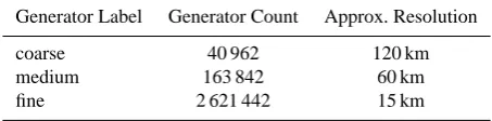
Table 1. Description of generator count labels, along with

approxi-mate grid resolution on an earth sized sphere.

Generator Label Generator Count Approx. Resolution coarse 40 962 120 km medium 163 842 60 km fine 2 621 442 15 km

3.3 Application to the construction of spherical centroidal Voronoi tessellations (SCVTs)

The parallel CVT construction algorithm of Sect. 2.2 is eas-ily adapted for the construction of centroidal Voronoi tessel-lations on the sphere (SCVTs). Obviously, one uses the sphe-rical version of the Delaunay triangulation algorithm as given in Sect. 3.2 instead of the version of Sect. 2.1. One also has to deal with the fact that if one computes the centroid of a sphe-rical Voronoi cell using Eq. (2), then that centroid does not lie on the sphere; a different definition of a centroid has to be used (Du et al., 2003a). Fortunately, it is shown in Du et al. (2003a) that the correct centroid can be determined by using Eq. (2), which yields a point inside the sphere, and then pro-jecting that point onto the sphere (actually, this was shown to be true for general surfaces) so that the correct spherical centroid is simply the intersection of the radial line going through the point determined by Eq. (2) and the sphere.

4 Results

All results are created using a high performance computing (HPC) cluster with 24 AMD Opteron “model 6176” cores per node and 64 GB of RAM per node.

Results are presented for three different generator counts, and are presented with the labels “coarse”, “medium”, and “fine”. Table 1 can be used to refer these labels to actual counts as well as approximate resolution on an earth sized sphere.

We use STRIPACK (Renka, 1997), a serial Fortran 77 As-sociation of Computing Machinery (ACM) Transactions on Mathematical Software (TOMS) algorithm that constructs Delaunay triangulations on a sphere, as a baseline for com-parison with our approach. It is currently one of the few well-known spherical triangulation libraries available.

(8)

4.1 Delaunay triangulations of the full sphere

Table 2 compares MPI-SCVT with STRIPACK for the con-struction of spherical Delaunay triangulations. The results given compare the cost to compute a single triangulation of a medium resolution global grid. The results show, for the computation of a full spherical triangulation MPI-SCVT is roughly a factor of 7 slower than STRIPACK in serial mode, and a factor of 12 faster when using 96 processors.

4.2 Initial generator placement and sorting heuristics for SCVT construction

We now examine the effects of initial generator placement and sorting heuristics with regards to SCVT generation. The results of this section are intended to guide decisions about which initial condition or sorting method we use later to gen-erate SCVTs.

4.2.1 Initial generator placement

Because most climate models are shifting towards global high-resolution simulations, we begin by exploring the cre-ation of a fine resolution grid. We compare SCVT grids constructing starting with uniform Monte Carlo and bisec-tion initial generator placement. The times for these grids to converge to a tolerance 10−6 in the`2norm are presented.

The 10−6threshold is the strictest convergence level that the Monte Carlo grid can attain in a reasonable amount of time, and is therefore chosen as the convergence threshold for this study. However, the bisection grid can converge well beyond this threshold in a similar amount of time. Table 3 shows timing results for the parallel algorithm for the two differ-ent options for initial generator placemdiffer-ent. Although the time spent converging a mesh with Monte Carlo initial placements is highly dependent on the initial point set, it is clear from this table that bisection initial conditions provide a significant speedup in the overall cost to generate an SCVT grid. Based on the results presented in Table 3 and unless otherwise spec-ified, only bisection initial generator placements are used in subsequent experiments. Bisection initial conditions are not specific to this algorithm, and can be used to accelerate any SCVT grid generation method.

4.2.2 Sorting of points for assignment to processors

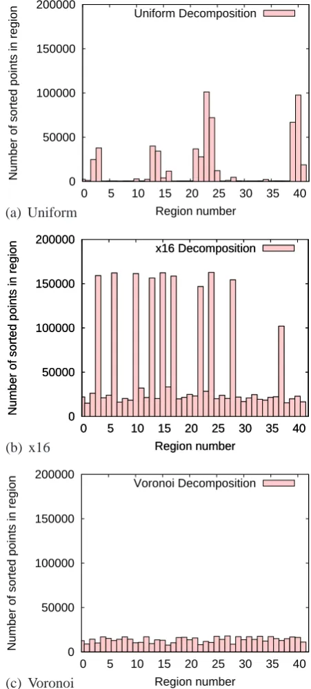
As described in Sect. 2.1.1, the MPI-SCVT code utilizes two methods for determining a region’s point set. Whereas the dot product sort method is faster, it provides poor load balanc-ing in variable resolution meshes, thus causbalanc-ing the iteration cost to be greater. Timings using both approaches are given in Table 4. Figure 3 shows the number of points that each processor has to triangulate on a per iteration basis. Tim-ings presented are for a medium resolution grid, 42 regions, 42 processors, and are averages over 3000 iterations. Three sets of timings are given. Timings labeled Uniform and×8

it not only speeds up the overall cost per iteration, but also provides a more balanced loads across

365 the processors. Note that, in Table 3, timings are taken relative to processor number 0, and as can

be seen in Fig. 5(a), processor 0 has a very small load so the majority of its iteration time is spent

waiting for the processors with large loads to finish and catch up; this idling time is included in the

Communication column of the table.

Sorting

Costs Of Different Algorithm Steps

Cost Per

Approach

Triangulation

Integration

Communication

Iteration

Speedup

Uniform

14.9779

39.3149

2556.971

2611.35

Base

x16

104.793

276.681 1560.71

1965.56

1.32 Voronoi

98.5482

249.77

288.694

640.472

4.07 Table 3. Timings based on sorting approach used. Uniform uses a coarse quasi-uniform SCVT to define region

centres and their associated radii and sorts using maximum distance between centres and neighbouring centres.

x16 uses a coarse SCVT with a 16 to 1 ratio in grid sizes to effect the same type of sorting. Voronoi uses the

same x16 coarse SCVT grid to define regions centres and sorts using the neighbouring Voronoi cell-based sort.

0 50000 100000 150000 200000

0 5 10 15 20 25 30 35 40

Number of sorted points in region

Region number Uniform Decomposition (a) Uniform 0 50000 100000 150000 200000

0 5 10 15 20 25 30 35 40

Region number x16 Decomposition 0 50000 100000 150000 200000

0 5 10 15 20 25 30 35 40

Region number x16 Decomposition (b) x16 0 50000 100000 150000 200000

0 5 10 15 20 25 30 35 40

Region number Voronoi Decomposition

(c) Voronoi

Fig. 5. Number of points each processor has to triangulate. 5(a), 5(b), and 5(c) use the sorting approaches

corresponding to the three rows of Table 3. All plots were created with the same set of 163842 generators.

Based on the results in Table 3, the new Voronoi-based sorting approach is used for all subsequent

370

15 it not only speeds up the overall cost per iteration, but also provides a more balanced loads across

365 the processors. Note that, in Table 3, timings are taken relative to processor number 0, and as can

be seen in Fig. 5(a), processor 0 has a very small load so the majority of its iteration time is spent

waiting for the processors with large loads to finish and catch up; this idling time is included in the

Communication column of the table.

Sorting

Costs Of Different Algorithm Steps

Cost Per

Approach

Triangulation

Integration

Communication

Iteration

Speedup

Uniform

14.9779

39.3149

2556.971

2611.35

Base

x16

104.793

276.681 1560.71

1965.56

1.32 Voronoi

98.5482

249.77

288.694

640.472

4.07 Table 3. Timings based on sorting approach used. Uniform uses a coarse quasi-uniform SCVT to define region

centres and their associated radii and sorts using maximum distance between centres and neighbouring centres.

x16 uses a coarse SCVT with a 16 to 1 ratio in grid sizes to effect the same type of sorting. Voronoi uses the

same x16 coarse SCVT grid to define regions centres and sorts using the neighbouring Voronoi cell-based sort.

0 50000 100000 150000 200000

0 5 10 15 20 25 30 35 40

(c) Voronoi

Fig. 5. Number of points each processor has to triangulate. 5(a), 5(b), and 5(c) use the sorting approaches

corresponding to the three rows of Table 3. All plots were created with the same set of 163842 generators.

Based on the results in Table 3, the new Voronoi-based sorting approach is used for all subsequent

370 it not only speeds up the overall cost per iteration, but also provides a more balanced loads across

365 the processors. Note that, in Table 3, timings are taken relative to processor number 0, and as can

be seen in Fig. 5(a), processor 0 has a very small load so the majority of its iteration time is spent

waiting for the processors with large loads to finish and catch up; this idling time is included in the

Communication column of the table.

Sorting

Costs Of Different Algorithm Steps

Cost Per

Approach

Triangulation

Integration

Communication

Iteration

Speedup

Uniform

14.9779

39.3149

2556.971

2611.35

Base

x16

104.793

276.681 1560.71

1965.56

1.32 Voronoi

98.5482

249.77

288.694

640.472

4.07 Table 3. Timings based on sorting approach used. Uniform uses a coarse quasi-uniform SCVT to define region

centres and their associated radii and sorts using maximum distance between centres and neighbouring centres.

x16 uses a coarse SCVT with a 16 to 1 ratio in grid sizes to effect the same type of sorting. Voronoi uses the

same x16 coarse SCVT grid to define regions centres and sorts using the neighbouring Voronoi cell-based sort.

0 50000 100000 150000 200000

0 5 10 15 20 25 30 35 40

(c) Voronoi

Fig. 5. Number of points each processor has to triangulate. 5(a), 5(b), and 5(c) use the sorting approaches

corresponding to the three rows of Table 3. All plots were created with the same set of 163842 generators.

Based on the results in Table 3, the new Voronoi-based sorting approach is used for all subsequent

370

15

Fig. 3. Number of points each processor has to triangulate. (a), (b),

and (c) use the sorting approaches corresponding to the three rows of Table 4. All plots were created with the same medium resolution grid.

(9)

Table 2. Comparison of STRIPACK with serial and parallel versions of MPI-SCVT for computation of a full spherical triangulation.

Com-puted using the same initial conditions for a medium resolution grid.

Algorithm Processors Regions Time (ms) Speedup (STRIPACK/MPI-SCVT) STRIPACK 1 1 563.87 Baseline

MPI-SCVT 1 2 3 724.08 0.15

MPI-SCVT 2 2 2 206.06 0.26

MPI-SCVT 96 96 45.75 12.33

Table 3. Timing results for MPI-SCVT with bisection and Monte Carlo initial generator placements and the speedup of bisection relative to

Monte Carlo. Final mesh is fine resolution.

Timed Portion Bisection (B) Monte Carlo (MC) Speedup MC_B Total Time (ms) 112 890 358 003 000 3171.25 Triangulation Time (ms) 10 887 48 034 600 4412.11 Integration Time (ms) 30 893 66 374 400 2148.52 Communication Time (ms) 70 878 110 958 000 1565.47

Table 4. Timings based on sorting approach used. Uniform uses a coarse quasi-uniform SCVT to define region centres and their associated

radii and sorts using maximum distance between centres and neighbouring centres.×8 uses a coarse SCVT with a 8 to 1 ratio in grid sizes to effect the same type of sorting. Voronoi uses the same×8 coarse SCVT grid to define regions centres and sorts using the neighbouring Voronoi cell-based sort.

Sorting Decomposition Costs Of Different Algorithm Steps Cost Per

Approach Grid Triangulation Integration Communication Iteration Speedup Distance Uniform 14.53 37.62 1314.22 1396.53 Baseline Distance ×8 35.84 92.91 865.32 995.04 1.40 Voronoi ×8 16.71 86.24 177.55 305.85 4.56

Timings presented in Table 4 are taken relative to proces-sor number 0, and as can be seen in Fig. 3a, procesproces-sor 0 has a very small load which causes the majority of its iteration time being spent waiting for the processors with large loads to catch up; this idling time is included in the Communica-tion column of the table.

Table 4 and Fig. 3 show there is a significant advantage to the Voronoi based sort method in that it not only speeds up the overall cost per iteration, but also provides more balanced loads across the processors.

4.3 SCVT generation

We now provide both quasi-uniform and variable resolution SCVT generation results. The major contributor to the differ-ences in computational performance arises as a result of load balancing differences. Results in this section make use of the density function

ρ(xi)=

1 2(1−γ )

tanh

_β_{− |}_x

c−xi|

α

+1

+γ (6)

which is visualized in Fig. 4, wherexi is constrained to lie

on the surface of the unit sphere. This function results in relatively large value ofρ within a distanceβ of the point

xc, where β is measured in radians and xc is also

con-strained to lie on the surface of the sphere. The function

tran-results. This should provide appropriate load balancing when generating SCVT meshes. Using

this sorting method should result in quasi-uniform and variable resolution SCVT generation to be

comparable in terms of performance.

4.3 SCVT generation

We now provide both quasi-uniform and variable resolution SCVT generation results. The major

contributor to the differences in computational performance arises as a result of load balancing

dif-ferences. Results in this section make use of the density function

ρ

(

x

i

) =

1 2(1

−

γ

)

tanh

β

− |

x

_c

−

x

_i

|

α

+ 1

+

γ

(6)

which is visualized in Fig. 6, where

x

i

is constrained to lie on the surface of the unit sphere. This

375 function results in relatively large value of

ρ

within a distance

β

of the point

x

c

, where

β

is measured

in radians and

x

c

is also constrained to lie on the surface of the sphere. The function transitions

to relatively small values of

ρ

across a radian distance of

α

. The distance between

x

c

and

x

i

is

computed as

|

x

c

−

x

i

|

= cos

−1

(

x

c

· x

i

)

with a range from

0 to

π

.

0 0.2 0.4 0.6 0.8 1

0 0.5 1 1.5 2 2.5 3

Density

Distance from centre of density function (Radians) Density Function

Fig. 6. Density function that creates a grid with resolutions that differ by a factor of 8 between the coarse and

the fine regions. The maximum value of the density function is 1 whereas the minimum value is

(1

/

8)

4

_.

Figure 7 shows an example grid created using this density function, with

x

c

set to be

φ

_c

= 3

π/

2 ,

380 λ

c

=

π/

6 , where

φ

denotes longitude and

λ

latitude,

γ

= (1

/

8)

4

,

β

=

π/

6 , and

α

= 0

.

20 with 10,242

generators. This set of parameters used in (6) is referred to as x8. The quasi-uniform version is

referred to as x1.

Fig. 4. Density function that creates a grid with resolutions that

dif-fer by a factor of 8 between the coarse and the fine regions. The maximum value of the density function is 1 whereas the minimum value is(1/8)4.

sitions to relatively small values of ρ across a radian dis-tance ofα. The distance betweenxc andxi is computed as

|xc−xi| =cos−1(xc·xi)with a range from 0 toπ.

Figure 5 shows an example grid created using this density function, withxc set to beλc=3π/2, φc=π/6, where λ

denotes longitude andφlatitude,γ=(1/8)4,β=π/6, and

(10)

1362 D. W. Jacobsen et al.: Parallel algorithms for Delaunay construction 8 D. W. Jacobsen et al.: Parallel algorithms for Delaunay construction

(a) Coarse region (b) Transition region

(c) Fine region

Fig. 7. Different views of the same variable resolution grid created using the density function (6). Figure 7(a)

shows the coarse region of the grid, 7(b) shows the transition region, and 7(c) shows the fine region.

In Sect. 4.1, we showed that MPI-SCVT performs comparably to STRIPACK when computing a

single full triangulation. However, computing a full triangulation is only part of the story. For SCVT

385

generation, a triangulation needs to be computed at every iteration of Lloyd’s algorithm as described

in Sect. 2.3. When using STRIPACK, the full triangulation needs to be computed at every iteration,

but with MPI-SCVT only each regional triangulation needs to be computed at each iteration. This

means the merge step can be skipped resulting in significantly cheaper triangulations.

Figure 8 shows the performance of a STRIPACK-based SCVT construction as the number of

390

generators is increased through bisection as mentioned in Sect. 2.3. Values are averages over 2000

iterations. The green dashed line represents the portion of the code that computes the centroids of

the Voronoi regions whereas the red solid line represent the portion of the code that computes the

Delaunay triangulation.

17

(a) Coarse region (b) Transition region

(c) Fine region

Fig. 7. Different views of the same variable resolution grid created using the density function (6). Figure 7(a)

shows the coarse region of the grid, 7(b) shows the transition region, and 7(c) shows the fine region.

In Sect. 4.1, we showed that MPI-SCVT performs comparably to STRIPACK when computing a single full triangulation. However, computing a full triangulation is only part of the story. For SCVT

385

generation, a triangulation needs to be computed at every iteration of Lloyd’s algorithm as described in Sect. 2.3. When using STRIPACK, the full triangulation needs to be computed at every iteration, but with MPI-SCVT only each regional triangulation needs to be computed at each iteration. This means the merge step can be skipped resulting in significantly cheaper triangulations.

Figure 8 shows the performance of a STRIPACK-based SCVT construction as the number of

390

generators is increased through bisection as mentioned in Sect. 2.3. Values are averages over 2000 iterations. The green dashed line represents the portion of the code that computes the centroids of

the Voronoi regions whereas the red solid line represent the portion of the code that computes the Delaunay triangulation.

17

Fig. 5. Different views of the same variable resolution grid created using the density function Eq. (6). (a) shows the coarse region of the grid, (b) shows the transition region, and (c) shows the fine region.

Table 2. Comparison of STRIPACK with serial and parallel versions of MPI-SCVT for computation of a full spherical triangulation.

Com-puted using the same initial conditions for a medium resolution grid.

Algorithm Processors Regions Time (ms) Speedup (STRIPACK/MPI-SCVT) STRIPACK 1 1 563.87 Baseline

MPI-SCVT 1 2 3 724.08 0.15

MPI-SCVT 2 2 2 206.06 0.26

MPI-SCVT 96 96 45.75 12.33

1.0e+00 1.0e+01 1.0e+02 1.0e+03 1.0e+04 1.0e+05

1.0e+02 1.0e+03 1.0e+04 1.0e+05 1.0e+06 1.0e+07

Average Time (ms)

Number of Generators

Triangulation Integration

Fig. 6. Timings for STRIPACK-based SCVT construction for

var-ious generator counts. Red solid lines represent the time spent in STRIPACK computing a triangulation whereas green dashed lines represent the time spent integrating the Voronoi cells outside of STRIPACK in one iteration of Lloyd’s algorithm.

steps, where the italicized steps are the ones added to the al-gorithm of Sect. 2.1:

– define overlapping spherical capsUk,k=1, . . . , N, that cover the given regionon the sphere;

– sort the given point set P into the subsets Pk, k= 1, . . . , N, each containing the points inP that are inUk;

1.0e-02 1.0e-01 1.0e+00 1.0e+01 1.0e+02 1.0e+03 1.0e+04 1.0e+05 1.0e+06

1.0e+01 1.0e+02 1.0e+03 1.0e+04 1.0e+05 1.0e+06 1.0e+07

Average Time (ms)

Triangluation Integration Communication

Fig. 7. Timings for various portions of MPI-SCVT using 2

pro-cessors and 2 regions. As the problem size increases the slope for both triangulation (red-solid) and integration (green-dashed) remain roughly constant.

– fork=1, . . . , N, construct in parallel the point setPke

by stereographically projecting the points inPkonto the

plane tangent to the sphere at the pointtk;

– fork=1, . . . , N, construct in parallel the planar Delau-nay triangulationTek of the points setPek;

03 19 Aug 2013

by: Douglas.

Fig. 5. Different views of the same variable resolution grid created using the density function Eq. (6). (a) shows the coarse region of the grid, (b) shows the transition region, and (c) shows the fine region.

Table 5. Comparisons of SCVT generators using STRIPACK, serial MPI-SCVT, and parallel MPI-SCVT. Cost per triangulation and iteration

are presented. Speedup is compared using the cost per iteration. Computed using the same initial conditions for a medium resolution grid. Variable resolution results are presented for MPI-SCVT only.

Algorithm Procs Regions Triangulation Iteration Speedup Per Iteration Time (ms) Time (ms) (STRIPACK/MPI-SCVT) STRIPACK 1 1 563.871 3 009.74 Baseline MPI-SCVT×1 1 2 3 480.43 9 485.78 0.32 MPI-SCVT×1 2 2 2 114.38 5 390.82 0.56 MPI-SCVT×1 96 96 14.23 207.26 14.52 MPI-SCVT×8 96 96 16.71 305.855 9.84

1.0e+00 1.0e+01 1.0e+02 1.0e+03 1.0e+04 1.0e+05

1.0e+02 1.0e+03 1.0e+04 1.0e+05 1.0e+06 1.0e+07

Average Time (ms)

Triangulation Integration

Fig. 6. Timings for STRIPACK-based SCVT construction for

var-ious generator counts. Red solid lines represent the time spent in STRIPACK computing a triangulation whereas green dashed lines represent the time spent integrating the Voronoi cells outside of STRIPACK in one iteration of Lloyd’s algorithm.

α=0.20 with 10 242 generators. This set of parameters used in Eq. (6) is referred to as×8. The quasi-uniform version is referred to as×1.

In Sect. 4.1, we showed that MPI-SCVT performs compa-rably to STRIPACK when computing a single full triangu-lation. However, computing a full triangulation is only part

1.0e-02 1.0e-01 1.0e+00 1.0e+01 1.0e+02 1.0e+03 1.0e+04 1.0e+05 1.0e+06

1.0e+01 1.0e+02 1.0e+03 1.0e+04 1.0e+05 1.0e+06 1.0e+07

Average Time (ms)

Fig. 7. Timings for various portions of MPI-SCVT using 2

pro-cessors and 2 regions. As the problem size increases the slope for both triangulation (red-solid) and integration (green-dashed) remain roughly constant.

(11)

1.0e-02 1.0e-01 1.0e+00 1.0e+01 1.0e+02 1.0e+03 1.0e+04

1.0e+02 1.0e+03 1.0e+04 1.0e+05 1.0e+06 1.0e+07

Average Time (ms)

Fig. 8. Same information as in Fig. 7 but for 96 processors and

96 regions.

Figure 6 shows the performance of a STRIPACK-based SCVT construction as the number of generators is increased through bisection as mentioned in Sect. 2.2. Values are aver-ages over 2000 iterations. The green dashed line represents the portion of the code that computes the centroids of the Voronoi regions whereas the red solid line represent the por-tion of the code that computes the Delaunay triangulapor-tion.

Table 5 compares STRIPACK with the triangulation rou-tine in MPI-SCVT that is called on every iteration. The re-sults presented relative to MPI-SCVT are averages over 2000 iterations.

As a comparison with Fig. 6, in Figs. 7 and 8 we present timings made for MPI-SCVT for two and 96 regions and pro-cessors, respectively, as the problem size, i.e. the number of generators, increases. A minimum of two processors are used because the stereographic projection used in MPI-SCVT has a singularity at the focus point.

Whereas Fig. 7 shows performance similar to that of STRIPACK (see Fig. 6), Fig. 8 shows roughly two orders of magnitude faster performance relative to STRIPACK. As mentioned previously, this is only the case when creating SCVTs as the full triangulation is no longer required when computing a SCVT in parallel.

4.4 General algorithm performance

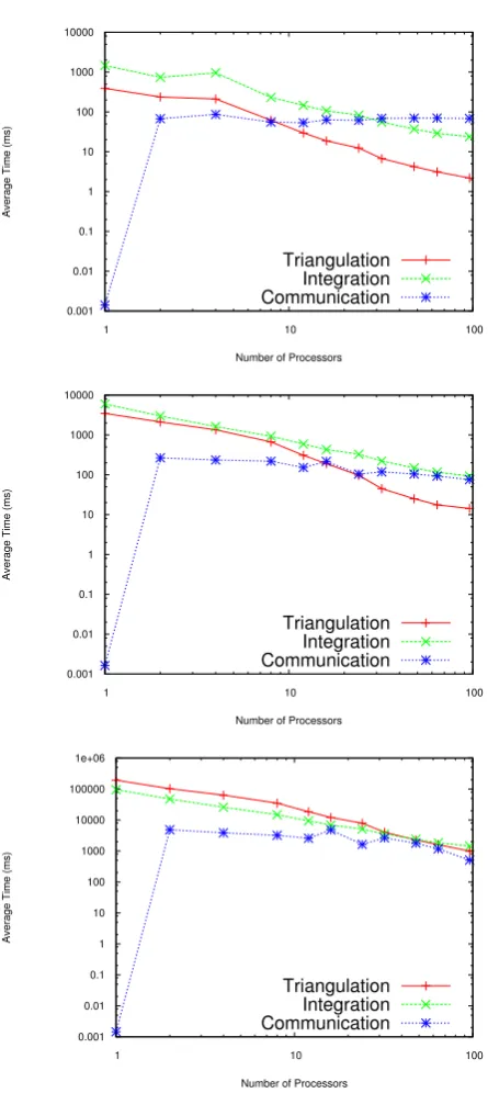
This section is intended to showcase some general perfor-mance results of MPI-SCVT. Figure 9a–c show the timings for a coarse resolution grid, a medium resolution grid, and a fine resolution grid, respectively.

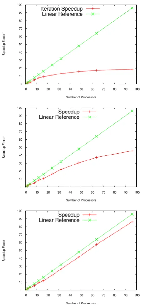
To assess the overall performance of the MPI-SCVT algo-rithm, scalability results are presented in Fig. 10. Figure 10a shows that this algorithm can easily under-saturate proces-sors; when this happens, communication ends up dominat-ing the overall runtime for the algorithm which is seen in Fig. 9a; as a result, scalability ends up being sub-linear. As

0.001 0.01 0.1 1 10 100 1000 10000

1 10 100

Average Time (ms)

Number of Processors

Triangulation Integration Communication

0.001 0.01 0.1 1 10 100 1000 10000

1 10 100

Average Time (ms)

Triangulation Integration Communication

0.001 0.01 0.1 1 10 100 1000 10000 100000 1e+06

1 10 100

Average Time (ms)

Number of Processors Triangulation

Integration Communication

Fig. 9. Timing results for MPI-SCVT vs. number of processors for

three different problem sizes. Red solid-lines represent the cost of computing a triangulation, whereas green-dashed lines represent the cost of integrating all Voronoi cells, and blue-dotted lines represent the cost of communicating each region’s updated point set to its neighbours.

(12)

0 10 20 30 40 50 60 70 80 90 100

Speedup Factor

Iteration Speedup Linear Reference

0 10 20 30 40 50 60 70 80 90 100

Speedup Factor

Number of Processors Speedup Linear Reference

0 10 20 30 40 50 60 70 80 90 100

Speedup Factor

Number of Processors Speedup Linear Reference

Fig. 10. Scalability results based on number of generators. Green is

a linear reference whereas red is the speedup computed using the parallel version of MPI-SCVT compared to a serial version.

neighbours. This is possible because points can only move within a region radius on any two subsequent iterations, and because of this can only move into another region which is overlapping the current region. More efficiency gains could be realized by improving communication and integration al-gorithms. This addition of shared memory parallelization to the integration routines might improve overall performance,

as the integration routines are embarrassingly parallel. Modi-fication of the data structures used could also enable the gen-eration of ultra-high resolution meshes (100M generators). In principle, because all of the computation is local this al-gorithm should scale linearly very well up to hundreds if not thousands of processors.

5 Summary

A novel technique for the parallel construction of Delau-nay triangulations is presented, utilizing unique domain de-composition techniques combined with stereographic pro-jections. This parallel algorithm can be applied to the gen-eration of planar and spherical centroidal Voronoi tessella-tions. Results were presented for the generation of sphe-rical centroidal Voronoi tessellations, with comparisons to STRIPACK, a well-known algorithm for the computation of spherical Delaunay triangulations. The algorithm presented in the paper (MPI-SCVT) shows slower performance than STRIPACK when computing a single triangulation in serial and faster performance when using roughly 100 processors. When paired with a SCVT generator, the algorithm shows additional speed up relative to a STRIPACK based SCVT generator.

Acknowledgements. We would like to thank Geoff Womeldorff and Michael Duda for many useful discussions. The work of Doug Jacobsen, Max Gunzburger, John Burkardt, and Janet Peterson was supported by the US Department of Energy under grants number DE-SC0002624 and DE-FG02-07ER64432.

Edited by: R. Redler

References

Amato, N. and Preparata, F.: An NC parallel 3D convex hull algo-rithm, in: Proceedings of the ninth annual symposium on Com-putational geometry – SCG ’93, 289–297, May 1993.

Batista, V., Millman, D., Pion, S., and Singler, J.: Parallel geomet-ric algorithms for multi-core computers, Comp. Geom.-Theor. Appl., 43, 663–677, 2010.

Bowers, P., Diets, W., and Keeling, S.: Fast algorithms for gen-erating Delaunay interpolation elements for domain decom-position, available at: http://www.math.fsu.edu/∼_{aluffi/archive/} paper77.ps.gz, (last access: May 2011), 1998.

Chernikov, A. and Chrisochoides, N.: Algorithm 872: parallel 2D constrained Delaunay mesh generation, ACM T. Math. Software, 34, 6:1–6:20, 2008.

Cignoni, P., Montani, C., and Scopigno, R.: DeWall: a fast divide and conquer Delaunay triangulation algorithm in E-d, Comput. Aided Design, 30, 333–341, 1998.

Du, Q. and Gunzburger, M.: Grid generation and optimization based on centroidal Voronoi tessellationss, Appl. Math. Comput., 133, 591–607, 2002.