Optimizing Virtual Backup Allocation for Middleboxes

Optimizing Virtual Backup Allocation for Middleboxes

Yossi Kanizo, Ori Rottenstreich, Itai Segall and Jose Yallouz

Abstract—In enterprise networks, network functions such as address translation, firewall and deep packet inspection are often implemented in middleboxes. Those can suffer from temporary unavailability due to misconfiguration or software and hardware malfunction. Traditionally, middlebox survivability is achieved by an expensive active-standby deployment where each middlebox has a backup instance, which is activated in case of a failure. Network Function Virtualization (NFV) is a novel networking paradigm allowing flexible, scalable and inexpensive implementation of network services. In this work we suggest a novel approach for planning and deploying backup schemes for network functions that guarantee high levels of survivability with significant reduction in resource consumption. In the suggested backup scheme we take advantage of the flexibility and resource-sharing abilities of the NFV paradigm in order to maintain only a few backup servers, where each can serve one of multiple functions when corresponding middleboxes are unavailable. We describe different goals that network designers can take into account when determining which functions to implement in each of the backup servers. We rely on a graph theoretical model to find properties of efficient assignments and to develop algorithms that can find them. Extensive experiments show, for example, that under realistic function failure probabilities, and reasonable capacity limitations, one can obtain 99.9% survival probability with half the number of servers, compared to standard techniques.

I. INTRODUCTION

Enterprise networks often rely on middleboxes to support a variety of network services such as Network Address Translation (NAT), load balancing, traffic shaping, firewall and Deep Packet Inspection (DPI). Typically, a middlebox is dedicated to implement solely a single function without a common standardization among different vendors, raising the complexity and cost of middlebox management.

Middlebox failures might occur frequently, inducing great degra-dation of service performance and reliability [2]. Failures might occur due to several reasons, such as connectivity errors (e.g., link flaps, device unreachability, port errors), hardware faults (memory errors, defective chassis), misconfiguration (wrong rule insertion, configuration conflicts), software faults (reboot, OS errors) or ex-cessive resource utilization. Temporary inability to support network functions can lead to packet drops, reset of connections, redundant packet delays, and in some cases even to security issues. A common approach for achieving middlebox reliability is through redundancy, where an additional instance of each middlebox operates as a backup upon a failure of the first [3], [4]. This approach is often referred to as active-standby deployment, where one (the “active”) instance handles all the traffic, while a second (the “standby”) instance is mostly inactive, until a failure occurs. Once a failure A preliminary version of this article appeared in the IEEE International Confer-ence on Network Protocols (ICNP) ’16, Singapore, November 2016 [1].

Yossi Kanizo is with the department of Computer Science, Tel-Hai College ([email protected]). Ori Rottenstreich is with the department of Computer Sci-ence, Princeton University, NJ, USA (e-mail: [email protected]). Itai Segall is with Bell Labs, Nokia ([email protected]). Jose Yallouz is with the department of Electrical Engineering, Technion ([email protected]).

is identified, all traffic is diverted to the standby instance, which has to immediately handle the functionality of the active one. While this approach enables simple dealing with a failure in each of the active middleboxes, it is often too restrictive and demands excessive redundancy in practice, especially since the frequency of failures can vary for different middleboxes, in addition to that usually not all the middleboxes encounter problems concurrently. Therefore, a milder and more flexible survivability approach is called for, which would relax the rigid requirement of an entire dedicated copy per active function.

Network Function Virtualization (NFV) [5] is a rising paradigm by which network functions are executed on commodity servers managed by a centralized software defined mechanism. Such virtual middleboxes are often also referred to as Virtual Network Functions (VNFs). By its elastic nature, NFV can considerably reduce operat-ing expenses. Specifically, we show how the flexibility of NFV can be utilized for planning of efficient backup schemes for running functions, while better utilizing resources to support recovery from failures.

A significant cost reduction can be achieved through sharing of resources among the standby instances of the different functions. Implementing the active-standby approach in NFV would require holding a virtual machine (VM), or an otherwise dedicated set of resources, for the standby copy of each function. For generality, we refer to this VM or set of resources as a server in this paper. Note that this does not necessarily refer to a physical server. Our suggested backup solution consists of multiple such servers, with a typical number smaller than the number of existing middleboxes. The proposed solution relies on the observation that while each such server is equipped with the resources required to run a single function, acting as a standby copy requires less resources. Therefore, a server is assumed to have the capability to backup several functions, namely some specific selected subset of functions. As soon as a failure occurs, a server is turned into an active instance of the function of the failed middlebox, discarding the other backup capabilities of that server. Note that as a standby machine, the server can backup multiple functions. Once becoming active, only one of those functions can be served by this server. We show that while causing a very low penalty in terms of survivability, our suggested backup scheme enables a significant reduction in the amount of required resources in comparison with the conventional active-standby approach.

server  S1  

LB  

DPI  

FW  

NAT  

  network    

func:ons   backup  servers  virtualized    

LB   NAT   IDS  

1                          2                  c=3      

IDS  

server  S2   LB   DPI   IDS  

1                          2                  c=3      

server  S3   LB   FW   NAT  

1                          2                  c=3      

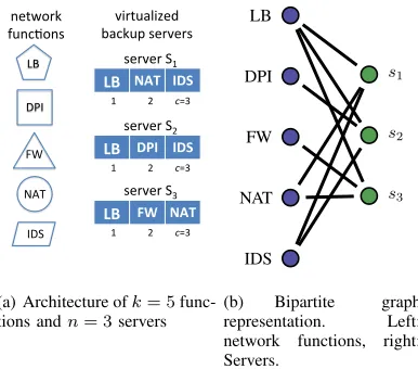
(a) Architecture ofk= 5 func-tions andn= 3servers

LB

DPI

FW

NAT

IDS

s1

s2

s3

(b) Bipartite graph representation. Left: network functions, right: Servers.

Fig. 1. (a) Illustration of architecture for middlebox survivability. A server can be used to backup one ofc= 3predetermined functions. To do so, the server must be frequently synchronized about the state of each of the functions it can backup. (b) Bipartite graph representation of the assignment of functions to servers. The degree of a server node is restricted to the capacityc.

increase in terms of diversity and complexity as middlebox vendors try to specialize their products. Thus, despite being in a standby mode, the number of functions that can be backed up by a server, staying in standby to replace any one of them, is limited and is expected to remain relatively low.

Network management under this aggregated standby mode should consider an important decision, namely the selection of the set of functions to be backed up in each of the servers. We demonstrate how this assignment affects the backup capabilities, and determines the possible combination of middlebox failures that can be resolved. Recall that in the case of two functions with faulty middleboxes, a single server that supports both functions cannot run more than one of them. In this work, we focus on aiming to optimize the backup scheme for maximum survivability under a given resource allowance. We detail several metrics describing goals that a network manager should take into account to achieve better survivability utilizing the constrained amount of resources.

Fig. 1(a) illustrates such a survivability architecture with five functions and three servers for backup. Each of the servers keeps the updated information required to recover three of the functions. In this example, for the load balancing function (LB), for instance, there is a backup in all the three servers and accordingly it can be recovered by any of them while for the deep packet inspection function (DPI) there is a backup in only one of the servers. Of course, information regarding the failure models and in particular their failure probabilities can be considered in the assignment of functions to servers to achieve higher survivability.

We investigate how to provide the best survivable solution supported by this approach of shared resources. To that end, we formalize two optimization problems describing possible goals that a network manager would often like to achieve in Section II. These problems consider the probability of full recovery from failures, as well as the expected number of functions that are available following a set of failures and the recovery process. In Section III and Section IV we establish fundamental properties of the problems while relying on tools from graph theory. We describe characteris-tics of optimal solutions, and show bounds on the performance of

optimal solutions. We show a family of instances for which the two problems collide, having the same set of optimal solutions but prove that the problems differ in the general case. We demonstrate that both problems are NP-hard by mapping different families of their instances to the known NP-hard number partitioning problem. Then, based on this analysis, we provide in Section V several algorithms to find efficient assignments. In Section VI we further discuss our findings about the problems. We study providing guarantees on the performance of the solutions, how to calculate the value of an assignment and provide formal descriptions of the optimization problems. In Section VII we demonstrate the advantages of our solutions through comprehensive simulations. Related work can be found in Section VIII. Finally, Section IX summarizes our results and discusses directions for future work. For space constraints, some proofs are omitted and can be found in [1].

II. MODEL ANDPROBLEMDEFINITION

We analyze this backup scheme through a graph framework. We denote the set of all functions byF and their number byk=|F|

such that F = {f1, . . . , fk}. Likewise, let n be the number of

servers and let c be the constrained capacity of a server, i.e., the maximal number of functions it can support. We refer to the set of servers by S satisfying |S| = n. We view an instance of the model as a bipartite graphFS_S

withk+nnodes. The assignment of functions to servers determines its edges. An edge between a server to a function illustrates the support of the function by the server. Fig. 1(b) shows the bipartite graph that corresponds to the assignment from Fig. 1(a). The capacity of the server limits its degree to at mostcwhile the degree of a function equals the number of servers implementing it with a value in [0, n].

A function fi ∈ F is associated with a failure probability pi.

We assume that these probabilities are mutually independent as well as that servers are always operational, i.e. do not encounter failures. These probabilities determine the possibility for every set of functions to be the set of faulty functions.

LetH ⊆Fbe the set of functions with a failure. Given such a set of functionsH, we are often interested in the induced graph of the set of faulty functionsH, their outgoing edges and the connected set of servers. Operational functions do not have to be recovered. A matchingM, representing a subset of the edges of the bipartite that corresponds to the assignment, describes the possibility to recover

|M| of the functions inH, such that a function can be recovered by its matched server. A matching of size|M|=|H|would enable recovering all faulty functions.

Consider for instance the functions and assignment from Fig. 1. Assume that the functions LB, FW and NAT encounter a failure while the functions DPI and IDS are operational. In this caseH = {LB, FW, NAT} ⊆ F and |H| = 3. For such a set H we can find a matching M in the bipartite from Fig. 1(b) of the form

M = {LB−s2,FW−s3,NAT−s1}. Since |M| = |H| = 3

we can recover all the three failing functions such that a function is recovered by its matched server, e.g., the function LB by the servers2. For a set of failing functionsH for which a matching of

size|H|cannot be found, it is impossible to recover all the failing functions.

model, to quantify the performance of the backup mechanism. Following the distribution of the set of faulty functions we can examine the probability for specific events or concentrate on other characteristics calculated on expectation. Ideally, we would like to verify that all functions have an operational instance. This would enable to successfully serve all traffic, regardless of the network functions that a specific flow requires to apply. In interesting scenarios the number of backup servers is smaller than that of the functions and it is thus impossible to guarantee that all functions are operational or can be recovered. To that end, we would like to maximize the probability of the scenario that all functions have an operational instance, as expressed in the first optimization problem studied in this work.

Problem 1. Given are a set of functions F with function failure

probabilities, a number of servers n, each with capacity c. The aim is to find an assignment that maximizes the probability for a recovery of all faulty functions. In such a recovery, each server is matched to at most one failed function, and each failed function is matched to one server.

We denote byPOP T the optimal, maximal possible probability.

Finding an optimal assignment that maximizes the probability for a recovery of all faulty functions is often very challenging. Moreover, in many cases, merely evaluating a solution, i.e. given a backup scheme – an assignment of functions to servers, calculating the probability for full recovery for this assignment can be a difficult task that requires considering a large number of combinations of faulty functions.

Sometimes there exists a benefit from a partial recovery of the faulty functions. In security applications for instance, availability of part of the security functions can increase the achievable level of defense. The Snort intrusion detection system [8] defines the notion of severity level where rules are categorized into levels such that examining a subset of them can be helpful. More generally, this partial recovery can be useful to serve all service chains that do not include the non-recovered functions. Similarly, a recent study [9] describes degrees of flexibility in the functions of a service chain, where a chain can be served with one among several functions or where the availability of some functions just contribute to improve the service quality or reduce the service time of service chains that can be completed with other functions. This motivates us in the definition of the following problem.

The next problem tries to maximize the number of available functions, i.e. the number of functions with operating middleboxes in addition to the maximal size set that can be recovered.

Problem 2. Given are a set of functions F with function failure

probabilities, a number of servers n, each with capacity c. The aim is to find an assignment maximizing the expected number of operating functions.

This problem is equivalent to trying to maximize the expected number of functions that are recovered. The two metrics differ by a constant, equal to the expected number of operating functions without the recovery. We denote by EOP T the optimal, maximal

expected number of operating functions.

In Section VI-D we provide a formal description of the two problems as optimization problems with target functions and a system of constraints. In both problems, finding a recovery is

performed for a given status of the middleboxes, i.e. indication which of them is not operating. In other words, we assume that all functions fail at once. When the assignment of functions to servers is known, as well as the set of failed functions, a recovery of a maximal number of failed functions, expressed by a matching in the induced graph, can be easily found (in polynomial time) using algorithms for maximum matching in bipartite graphs (e.g., [10], [11]). In case a failing function with an implementation in more than a single server, the servers should agree in which of them the function should be recovered. This can be achieved through an identical implementation of the matching algorithm by the different servers. Accordingly, while as mentioned a frequent synchronization between a function and its implementing server is crucial, an additional synchronization between the servers, e.g. to agree on the server used for recovery, is not required.

Along most of the paper, we follow the assumption that a server cannot recover simultaneously more than a single function. As mentioned in the introduction, we assume enough resources in each server to recover a single function. We later provide experiments examining the benefit of being able to recover within the same server more than a single failing function to study cases when this assumption can be relaxed.

Our model has several additional simplifying assumptions, often required for the analysis. First, it does not consider a potential correlation between failures of different functions. In addition, it assumes that all functions require the same capacity when being backed up by a server. The model also assumes that the physical location of a function implementation does not affect the performance. We discuss a possible dependency between failure probabilities in Section VI-E and leave model generalizations for future work.

III. PROBLEM1: FULLRECOVERYPROBABILITY In this section we address Problem 1. We aim to find an assignment that maximizes the probability that all functions are operational or can be recovered. While the problem is rather easy when each server has a capacity of 1, we show that for a larger capacity the general problem is NP-hard.

For the set ofkfunctionsF={f1, . . . , fk}let{p1, p2, . . . , pk}

be the respective function failure probabilities. W.l.o.g. assume functions have non-zero failure probabilities (a function that never fails does not require a backup) that are ordered in a non-decreasing order p1 ≤ p2 ≤ · · · ≤ pk, i.e., the earlier functions are more

reliable. Denote bypthe product of thosek probabilities. The set ofnservers is denoted byS={s1, s2, . . . , sn}, each with capacity c.

A simple observation is that it is impossible to guarantee a recovery of any combination of failed functions with less than

n = k servers. Due to the independence of functions, they can all fail together even if this scenario has a very small probability. It is also easy to guarantee that with at leastkservers by dedicating a server to each function.

Corollary 1. The optimal full recovery probability satisfies

POP T <1 when the number of servers isn < k and POP T = 1

whenn≥k.

A. Simple Case: c= 1

Theorem 2. In case c = 1, the optimal assignment of functions

to servers is by assigning the n servers with then functions with top failure probability, each server to a different function. Con-sequently, the optimal full recovery probability satisfies POP T =

Qk−n

i=1 (1−pi), i.e. the probability that all firstk−nfunctions do

not fail.

Proof. Once a function is recovered by some server, all other servers that are assigned to this function are useless (each server is assigned with only one function in our case). Therefore, all n

servers should be assigned to distinct functions. Then, the first part of the theorem easily follows. Finally, full recovery is achieved if and only if none of the otherk−nfunctions fail, which yields the second part of the theorem.

The simplicity of the case ofc= 1allows us to derive this result that does not hold for larger values ofc. For such larger values, in the decision of an assignment it is required to determine not only which functions would have backups but also how many backups each function should have. Furthermore, there is also an importance for deciding about instances of what functions would be assigned to the same server.

B. Problem Hardness

We now focus on the case wherec= 2. This case is much more complicated to analyze and to solve. In fact, a capacity of c = 2

suffices to show that the problem is NP-hard.

Our proof for the NP-hardness of this problem provides an intuition on how it can be solved approximately and inspired us in the design of the approach we take to tackle this problem later. The basic idea is to focus on the connected components of the underlying bipartite graph. In each connected component, nodes represent either servers or functions. To prove the following two properties we rely on [12]. The first property follows immediately from Lemma 1 there.

Property 3. In case c = 2, each connected component with t

servers has at most t+ 1 functions.

We also show the following.

Property 4. In casec= 2, letC be a connected component with

t servers andq≤t+ 1functions. Then for each subset of size (at most)min{t, q} of functions, there is a matching containing all of the functions.

Proof. If q≤t thenmin{t, q} =q. Then, by Lemma 2 in [12], the q functions have a matching of size q = min{t, q}. Thus, any subset of the functions has also a matching (using the same edges as in the matching of size q). Otherwise,q=t+ 1and so

min{t, q}=t. LetH ⊆F of sizet=q−1. We now show it has a matching of size |H|=t (and by the same argument as above any subset ofH has a matching).

LetFi be the only function inF\H, and consider the subgraph

induced byH and the server set. This subgraph containstfunctions andtservers, and has one or more connected component. We show that for each such connected component the number of functions equals the number of servers. Assume on the contrary that some connected component has a number of function that is not equal

to the number of servers, and consider a connected component for which the number of functions is larger than the number of servers. Such a connected component must exist since the number of functions inH equals the number of servers (in H).

Let a be the number of servers in this connected component. By the connectivity of G, function Fi must be connected to one

of those a servers. Thus, the number of functions connected to thoseaservers is at least a+ 2. By Property 3 such a case cannot exist. Therefore, all connected components inH have a number of functions that is equal to the number of servers, and by Lemma 2 in [12] have a perfect matching each, implying that the maximum matching size ofH ist.

The next theorem is easily followed:

Theorem 5. In casec= 2, and n < k, i.e., the number of servers is lower than the number of functions, each connected component in an optimal solution contains a number of functions that is larger by one than the number of servers.

Proof. Consider an optimal solution. Sincen < k there is at least one component with a number of servers smaller than the function number by exactly one. Difference cannot be larger by Property 3. We denote one such component byC1. If the current theorem does

not hold, there exists a second componentC2withtservers andq≤ tfunctions. We show that the two components can then be merged to increase the probability for recovery of all failing functions, in contradiction to the optimality of the solution.

By Property 4 all functions inC1can be recovered as long as not

all of them fail together. We say then that the survival probability of the component is1−PC1 = 1−

Q

i∈FC1pi. Similarly, by the same property, we can always recover any set of failing functions fromC2, even if they all fail. Thus all functions inC1, C2 can be

recovered with probability1−PC1.

For an arbitrary spanning tree of C2, consider an edge of the

connected component that is not included in the tree. Since there arec·t= 2tedges, there must be such an edge not included in the at mostt+q−1≤2t−1edges in the spanning tree. Omitting this edge does not eliminate the connectivity ofC2. We can therefore

merge the two components C1, C2 by connecting one such edge

to an arbitrary function in C1, without changing the server it is

connected to. Then, we obtain one connected componentCinstead of the twoC1, C2, witht0servers andq0≤t0+1functions. Failures

within its functions can be fully recovered with probability 1−

PC= 1−Q_i∈FCpi= 1−Q_i∈FC

1 S_F

C2pi>1−

Q

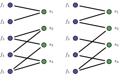
i∈FC1pi, i.e., larger than before the merge operation. Recovery probabilities for the other connected components are not affected by the change. Such a change is illustrated in Fig. 2 (for an arbitrary order of the functions) where in (a) there are two connected components C1

with functions{f1, f2} and a single server andC2 with functions {f3, f4, f5} and three servers. In (b), by changing a single edge

betweens2 to functionf2 instead of f3, the number of connected

components is reduced to one, improving the survival probability.

f1

f2

f3

f4

f5

s1

s2

s3

s4

(a) non-optimal assignment I, 2 connected components

f1

f2

f3

f4

f5

s1

s2

s3

s4

(b) optimal assignment II, a sin-gle connected component

Fig. 2. Illustration of the structure of the bipartite graph in an optimal assignment forc= 2(Theorem 5). Left: network functions. Right: Servers. Survival probability is improved when reducing the number of connected components as in a transition from (a) to (b) with the change of a one edge.

Theorem 6. In casec = 2, andn < k, the number of connected

components in an optimal solution is k−n. This is the minimal possible number of components under these assumptions.

We now turn to compute the survival probability of a connected component.

Theorem 7. In case c = 2, and n < k. Let C be a connected

component in an optimal assignment, and let {g1, . . . , gq} be the

set of all function indices inC. Then the survival probability of the connected component is given by1−Qq

i=1pgi.

Proof. By Theorem 5 we get that the number of functions in

C is t+ 1 while the number of servers is t, for some t ∈ N.

Therefore, for each subset of functions of sizetthere is a matching in C (Property 4). Consequentially, the only case where not all functions can be recovered is the case where all of them fail. This happens with probabilityQq

i=1pgi. The survival probability follows

by taking the complement.

Next, one may compute the overall survival probability, which is given by the product of the survival probability of all connected components. This follows immediately from the independence of function failure probabilities.

Theorem 8. The overall survival probability is given by the product of all connected component survival probabilities.

Note that the last theorem is valid also for arbitrary values

of c, n, k. We begin to have a clear picture on how an optimal

assignment looks like, as an intuition on how to split the connected components in the graph. Informally, we would want the connected components’ survival probabilities to be balanced. We start with the special case where an optimal solution has two connected components.

Intuitively, there is a dependency between functions within the same connected component such that it might be impossible to recover one upon some scenario of others. Consider two functions

i, j with failure probabilitiespi> pj. Assume their backup should

be selected from two available server slots, each translated to adding the function to one of two connected components C1, C2 with

current failure probabilitiesPC1> PC2. Since functionifails more

often, we wish to prioritize it. Thus it would be better to place it in the connected component with more reliable existing functions, i.e. in C2. The other function, j, which encounters failures less

frequently, will be placed in C1 with existing functions that are

more failure-prone. This addition will contribute to the balancing of the two failure probabilities of the two connected components.

Theorem 9. In casec= 2, andk=n+2, the optimal solution has

exactlytwo connected components. Among all possible assignments such that the bipartite graph has two connected components C1

andC2with respective connected component survival probabilities 1 −PC1 and 1 −PC2, the optimal assignment is the one for

which max{PC1,PC2}

min{PC1,PC2}

is minimized. In particular, if PC1 = PC2

the assignment is optimal.

Proof. First, since k = n+ 2, by Theorem 6 the number of connected components is k−n= 2. LetA be an assignment that results in two connected components C1 and C2 with respective

connected component survival probabilities1−PC1 and1−PC2. Also, let r = max{PC1,PC2}

min{PC1,PC2}

. Assume that there exists an assign-ment A0 with the corresponding C10, C20, 1−PC01, 1−P

0 C2, and

r0 = max{P

0

C₁,P

0

C₂}

minnP0

C1,P

0

C2

o, such that r

0 _{< r. Since there exist exactly}

two connected components in each assignment, a function not included in one component must be included in the second and

C1\C10 =C20\C2 andC2\C20 =C10 \C1.

We will show that the survival probability of the assignmentA0

is larger than the corresponding probability of the assignment A, i.e. that(1−P_C0

1)(1−P

0

C2)>(1−PC1)(1−PC2).

To show this, we assume w.l.o.g. that PC1 ≥ PC2 and P

0 C1 ≥

P_C0

2. This implies that

PC1

PC2

>P 0

C1

P0

C2 .

We define α = PC1∩C01 and β = PC2∩C20. In words, α is the product of probabilities of the functions that are assigned to the first connected component in both solutions, and similarly β for the second component.

We further define a = PC1\C10 = PC20\C2 and b = PC2\C20 =

PC0

1\C1. That is, ais the product of probabilities of the functions that are assigned to the first connected component in the solution

A, but not to the first in A0. Note that PC1 = a·α. Therefore,

PC0

2 =a·β. Symmetrically,PC2=b·β andPC10 =b·α.

PC1

PC2

>P 0 C1

P0 C2

⇒ aα

bβ > bα

aβ ⇒a

2_{> b}2_{⇒a > b}

P_C0

1≥P

0

C2 ⇒b·α≥a·β > b·β⇒α > β

By combining both of the above,a(α−β)> b(α−β)

⇒aα+bβ > bα+aβ

⇒PC1+PC2 > PC10 +PC20

⇒1 +p−PC0

1−PC02>1 +p−PC1−PC2

⇒(1−P_C0

1)(1−P

0

C2)>(1−PC1)(1−PC2).

larger failure probability. Similarly, a better balancing is achieved when the failure probability selected to be decreased is that of the component with a larger failure probability. The scenario this addition can make a difference is when the new function does not fail while all other functions in its connected component fail. The probability for that is maximized in a component with a larger failure probability.

By reducing the number partitioning problem [13] to our problem it is possible to show that the discussed problem is NP-hard. In the number partitioning problem, the goal is to divide a multiset of positive integers into two disjoint subsets while minimizing the absolute value of the difference of the subset sums.

Theorem 10. Finding an optimal assignment for Problem 1 is

NP-hard (even forc= 2).

While many of the results described in this section were sug-gested for c = 2, they often do not apply for larger values of c. We can easily extend the more simple of them for such values. We can show, for instance, similarly to Property 3, that in a connected component with tservers there are at mostc+ (t−1)·(c−1) =

t·(c−1) + 1functions. However, it seems impossible to derive a

similar complete analysis for such values. The reason is that while in the case ofc= 2we managed to express the survival probability of a connected component based only on its functions (Theorem 7), for c ≥3 this cannot be done. Often the survival probability of a component is not well defined by its number of servers and its functions and can be influenced by the internal structure of the component.

C. Bounds

In this section we describe an upper bound on the value of the optimal full recovery probabilityPOP T for the case ofc= 2.

We start with the following simple lemma.

Lemma 1. Foru1, u2, u3, u4satisfying0< u1< u2≤u3< u4< 1 and u2·u3=u1·u4. Then,u2+u3< u1+u4.

We can also suggest the following upper bound.

Theorem 11. In case c= 2, the optimal full recovery probability

satisfies POP T ≤

1−pk−1n

k−n

, where p = Qk

i=1pi is the

product of all function failure probabilities.

IV. PROBLEM2:EXPECTED NUMBER OF RECOVERED FUNCTIONS

Sometimes there can be a benefit from any available function that is running. In this section we study Problem 2, where we try to maximize the number of such functions, i.e. the functions with an operating middlebox together with the set of functions that can be recovered. We recall that we refer to the optimal (maximal) value of the expected number of such functions asEOP T.

We can easily observe thatEOP T increases for larger number of

serversnand thatEOP T =konly forn≥k(assumingpi>0), i.e.

when the number of servers equals at least the number of functions. A given assignment determines the connected components in the bipartite graph. Then, by the linearity of expectation the expected number of operating functions is given by the sum of their number in each connected component.

Problem 1 and Problem 2 are similar since in both problems it is more important to be able to recover a function that fails more frequently, i.e. with a larger failure probability. The difference comes from the fact that the first problem does not benefit from a partial recovery of the non-operating middleboxes. While we show that the problems coincide for some families of inputs we demonstrate that they differ in the general case.

A. Similarity of Problem 2 to Problem 1 and its NP-Hardness

The two problems collide for the casec= 2andk=n+ 2and their optimal solutions then coincide. This allows us to deduce that Problem 2 is also NP-hard. To show that we can rely on Property 3 and Property 4 that hold for general bipartite graphs (withc= 2).

Theorem 12. In a connected component C of t servers and q=

t+ 1 functionsFC, the expected number of operating functions in

this component isEC=q−Qi∈FCpi.

Similarly, Theorem 5 holds also for this problem. Also for this problem, it does not hold for c >2.

Theorem 13. In casec= 2, andn < k, i.e., the number of servers is lower than the number of functions, each connected component in an optimal solution to Problem 2 contains a number of functions that is larger by one than the number of servers.

By Theorem 13, we get that also for Problem 2, if c = 2 and

n < kin an optimal solution the number of connected components

isk−n.

It is possible to show that forc= 2, andk=n+ 2, the optimal solutions of Problem 1 and Problem 2 coincide.

Theorem 14. In case c = 2, and k = n+ 2, the set of (one or

more) optimal solutions is the same in Problem 2 and Problem 1.

Finally, based on the above one can deduce that Problem 2 is also NP-hard.

Theorem 15. Finding an optimal assignment for Problem 2 is

NP-hard (even forc= 2).

B. Bounds

We can derive an upper bound on the expected number of available functions.

Theorem 16. In case c = 2, the optimal expected number of

available functions satisfies EOP T ≤ k−(k−n)·p

1

k−n_{, where}

pis the product of all function failure probabilities.

C. Between the two optimization problems

Based on the similarity between Problem 1 and Problem 2 as we detailed, one might wonder whether the two problems are identical. It turns out that: a) the problems are very similar, and in the vast majority of cases, their optimum solutions coincide. This will be demonstrated further in Section VII, however: b) the problems are not identical. There exist cases where the optimal solutions for the two problems differ.

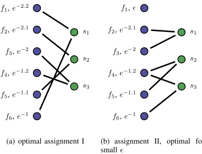
f1,e−2.2

f2,e−2.1

f3,e−2

f4,e−1.2

f5,e−1.1

f6,e−1

s1

s2

s3

(a) optimal assignment I

f1,

f2,e−2.1

f3,e−2

f4,e−1.2

f5,e−1.1

f6,e−1

s1

s2

s3

(b) assignment II, optimal for small

Fig. 3. Illustration of the distinction between Problem 1 and Problem 2 (Sec-tion IV-C). Left: network func(Sec-tions. Right: Servers. The failure probability appears for each function. When changing the failure probability of the first functionp1 frome−2.2_{to a small >0, the optimal assignments for each of the two problems} changes from assignment I (in (a)) to assignment II (in (b)).

and n = 3, c = 2, and first consider the failure probabilities be p1, . . . , p6 = e−2.2, e−2.1, e−2, e−1.2, e−1.1, e−1. An optimal

assignment to Problem 1 (assignment I) is with connected com-ponents C1 = {f1, f6}, C2 = {f2, f5}, C3 = {f3, f4} (achieved

for servers implementing functions {f1, f6},{f2, f5},{f3, f4}). It

achieves full recovery probability of POP T = (1 −p1 ·p6)·

(1−p2· p5)·(1−p3 ·p4) = (1 −e−3.2)3 = (1−p

1 3)3 for

p= Qk

i=1pi. The solution must be optimal since it achieves the

upper bound from Theorem 11. This is also an optimal solution for Problem 2 achieving an expected number of k−p1 ·p6 −p2 ·

p5−p3· p4 = 6−3 ·e−3.2 = k−(k−n)·p

1

k−n _available

functions as in the upper bound from Theorem 16. If we set

p1 = (i.e., arbitrarily small), for both problems, there is no

need to backup the first function and for both problems an optimal assignment (assignment II) has the connected components C0

1 = {f1}, C₂0 = {f2, f3}, C30 = {f4, f5, f6} (achieved for instance

for servers implementing functions {f2, f3},{f4, f5},{f4, f6}).

Moreover, for p1 ∈ [, e−2.2] the transition value of p1 between

the two optimal solutions is different for the two problems. For Problem 1 we compare (1−p1·p6)(1−p2·p5)(1−p3·p4) = (1−p1)(1−p2·p3)(1−p4·p5·p6) and get a transition point

of p2·p3−p2·p5−p3·p4+p4·p5·p6+p2·p3·p4·p5−p2·p3·p4·p5·p6

p6+p2·p3−p2·p5·p6−p3·p4·p6+p4·p5·p6−1 ≈0.044390. For Problem 2 we compare 6−p1· p6 −p2 ·p5−p3· p4 = 6 − p1 −p2 · p3 − p4 · p5 ·p6 and get a transition point of

p2·p3−p2·p5−p3·p4+p4·p5·p6

p6−1 ≈0.044404. Ifp1 is set to be between

the two transition points, we have different optimal solutions for the two problems. The two assignments are illustrated in Fig. 3.

V. SOLUTIONS

We suggest various approaches to tackle the two problems. Due to the similarity between the problems, as discussed in Section IV-C, the approaches are agnostic to the problem at hand, and compute a solution that is expected to be effective for either problem. The heuristics presented in this section rely on the intuition developed in previous sections. Specifically, from Theorems 6 and 9 (resp.), we extract a general guideline to: a) reduce the number of connected components as much as possible,

and b) keep the product of failure probabilities in the components as balanced as possible.

A. Simple Random Assignment (SRA)

The first approach is mainly used as a reference to the algorithms described in Section V-B and Section V-C.

In the SRA algorithm, we pick, randomly and independently, for each server c different functions that it backups, where the probability to choose any function is proportional to the specific function failure probability. The exact steps are described below:

• Compute the proportional probability vector defined by {p1, p2, . . . , pk}/Ppi.

• For each serversj, j∈[1, n]:

– Letvj=v.

– For each of the c backup slots: Randomly and indepen-dently pick a function using the distribution defined invj.

Updatevj by removing the function that was picked and

normalize back to a sum of 1.

B. Constrained Random Assignment (CRA)

Based on the intuitions obtained above we perform a slight modification to the SRA algorithm where the effect of the value of the failure probability of a function on the number of instances is moderate.

The basic idea is to decide in advance how many backups each function has, and then distribute the backups to the servers. The number of backups should be as even as possible, with a maximal difference of one. The exact steps are described below:

• Decide on the number of backupsbifor functionfi∈F. Start

withbn·c/kcbackups for each one. Add an extra backup to the functions with the top(n·c) mod kfailure probabilities.

• For each server sj ∈ S, select randomly c among the n·c

instances, avoiding multiple selections of the same function by the same server.

C. Balanced Assignment (BA)

The following approach is also based upon the intuitions from the analysis. It consists of three phases:

• Decide on the number of connected components. As was shown, a crucial aspect in the effectiveness of a backup scheme is the partitioning of the corresponding bipartite graph into connected components. Therefore, in the first phase we choose the number of such components to partition the graph into.

• Partition the functions into the connected components. As discussed, the aim is to partition the functions such that the product of failure probabilities for functions in each component is balanced.

• Construct the actual backup scheme, by assigning functions to servers.

1) Deciding on the number of connected components: General-izing on Theorem 6, we wish to minimize the number of connected components. Therefore, given k functions, and n servers with capacity c, we choose to construct t = max(1, k−(c−1)·n)

connected components.

2) Partitioning the functions into the connected components:

Generalizing on Theorem 9, the aim of the partitioning is to balance as much as possible the product of failure probabilities of functions in each partition. We choose a greedy approach to this problem. First, functions are sorted in non-decreasing order of their failure probability. Then, each function is assigned to the partition with the largest product of failure probabilities so far.

In order to allow a mapping of the functions in each partition to servers, that is consistent with the choice of t above, we require the size of each partition to be(c−1)·w+ 1for some integerw. If in the result of the greedy algorithm this is not the case, we shift functions between partitions. In order for this to affect the balance between the partitions the least, we choose to shift the functions with the highest failure probability.

3) Constructing connected components from the partitions: Each set of functions partitioned together in the previous step should now get a set of servers, and mapping between the functions and servers, such that a connected component is formed in the corresponding bipartite graph. Clearly, the construction of each component is independent of the other components, so we focus on a single given component.

Assuming the connected component consists off functions, let

z = f−1_c−1 be the minimal number of servers required in order to construct a connected component for these functions. We re-partition thef functions intoz partitions, under the constraint that no partition contains more thancfunctions, using the same greedy heuristics as before. Each such partition is then mapped to a single server. For each remaining backup slots, i.e. for each server that received less than c functions, we connect the functions with the maximal failure probability from the previous partitions until c

functions are backed up. This guarantees the connectivity within the component.

4) Assigning functions to remaining servers: For the case where all functions are grouped into a single connected component, i.e. whenk−(c−1)·n≤1, the number of servers,z, in the previous step, might be smaller than n. Then, we have servers that were not assigned to any function at this point. Leaving unused servers is not optimal, so to those servers not in use, we assign functions in decreasing order of failure probabilities. We skip the functions with highest probability, as they were already assigned an additional backup when connecting the component in the previous step.

VI. DISCUSSION

A. Approximation Guarantees

We notice that the balancing algorithm, presented in Section V-C above is a generalization of a greedy algorithm. For the special case of c = 2 and k −n = 2, where exactly two connected components are constructed, the algorithm is in fact the simple greedy algorithm that constructs two partitions by sorting the functions in non-decreasing order of their failure probability, and assigning each function to the partition with the largest product of failure probabilities so far.

optimal survival probability

0.9 0.97 0.99 0.999 0.9999 0.99999

survival probability 0.9 0.97 0.99 0.999 0.9999 0.99999

P_OPT

P_GREEDY

(a) Problem 1

optimal available functions 9.97 9.99 9.999 9.9999 9.99999 available functions 9.97

9.99 9.999 9.9999 9.99999

E_OPT E_GREEDY

(b) Problem 2

Fig. 4. Guarantees on the results of the greedy algorithm based on the optimal values. (a) Problem 1 withp= 10−10_{, (b) Problem 2 withp= 10}−10_{,k= 10.}

This algorithm is equivalent to applying the well-known greedy algorithm for number partitioning, on inputs equal to minus the log of failure probabilities, similar to the reduction in Theorem 10. This algorithm is known to achieve7/6approximation of the size of the larger partition [14]. One might ask how that known approximation ratio translates into guarantees on the effectiveness of the balancing algorithm, at least for this special case of c = 2 andk−n= 2. Unfortunately, the result does not imply a fixed approximation ratio, but enables us to derive bounds on the performance of the greedy algorithm that vary for different instances.

Assume an instance with p =Qk

i=1pi for failure probabilities p1, . . . , pk. Let PCo1, P

o

C2 be the product of failure probabilities of functions in the two connected components in an optimal solution such that POP T = (1−PCo1)·(1−P

o

C2) is the optimal survival probability. We derive PGREEDY, a lower bound on the survival

probability of the greedy solution.

We denote PC1, PC2 the products corresponding to the two connected components in the greedy solution. We assume w.l.o.g.

P_Co₁ ≥P_Co₂ andPC1 ≥PC2. They satisfyP

o C1·P

o

C2 =PC1·PC2 =

p. The 7/6 approximation ratio on the size of the larger partition in number partitioning gives us the following relation between

Po

C2 andPC2: PC2 ≥ (P

o C2)

7/6_{. HereP}o

C2 <1 and PC2 satisfies

(Po C2)

7/6 _≤P C2 ≤P

o

C2. For a given value ofPOP T we solve the two equations (1−Po

C1)·(1−P

o

C2) = POP T, P

o C1 ·P

o C2 = p to derive Po

C2. The minimal survival probability is obtained by the greedy algorithm when the lower bound on PC2 is tight and

PC2 = (P

o C2)

7/6_{. Then we can calculate P}

C1 = p/PC2 and

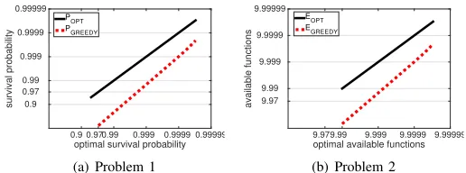
PGREEDY = (1−PC1)·(1−PC2)as a function ofp, POP T. In Fig. 4(a) we demonstrate this by setting a constantp= 10−10, and leavingPOP T, the survival probability of the optimal solution,

as an independent variable. We plot PGREEDY as a function of POP T for this case, as well as the identity function of POP T for

comparison. Several points can be observed:

• For low values ofPOP T, below roughly0.962724in this case,

the value of PGREEDY is negative (hence not plotted in this

figure). This means that the approximation is too loose to be of any value.

• Above a certain value ofPOP T, there is no real solution for

Po

C2, i.e., no real inputspi exist for this case. In our example withp= 10−10, no inputs exist for which POP T >1 +p−

2√p= 1 + 10−10−2·10−5≈0.99998.

• As POP T approaches its highest possible values, the ratio

between the bound on the probability of the greedy and the optimal one is improved (i.e., larger). For this example with

p= 10−10_{, the ratio is 0.9863 forP}

for POP T = 0.99997.

For Problem 2, very similar derivations apply. Here we need to assume as given, in addition topandEOP T, alsok, the number of

functions. We start fromEOP T =k−PCo1−P

o

C2, assume worst case values forPC2 and derive a formula for EGREEDY as a function of p,EOP T andk. Fig. 4(b) plots this forp= 10−10, k= 10.

B. Calculating the value of an assignment

The number of possible assignments can be large, i.e. exponential in the number of servers and their capacity c. Moreover, for both problems calculating the value of a given assignment, i.e. the survival probability in Problem 1 or the expected number of available functions in Problem 2 is not an easy task. The number of scenarios with different set of failing functions that have to be taken into account is 2k_{, i.e., exponential in the number of functions.}

This often restricts the number of functions we can consider in the experimental settings. We develop dynamic-programming based techniques to accelerate this calculation.

Our approach relies on the so called defect version of Hall’s theorem [15], also known as Ore deficiency theorem [16]. Given a bipartite graph G with bipartation (U, V), the deficiency of the graphG, is given by

def(G) = max

A⊆U{|A| − |D(A)|},

where the operatorD(A)extracts the set of neighbors of all vertices inA. The defect version of Hall’s theorem states that the maximum matching size of the graphGis exactly|U| −def(G).

We go over all function subsets ordered by their subset size, maintaining the deficiency of the graph induced by each subset, the probability that this subset of functions fail (and all other do not fail), and the set of neighbors. An update of the deficiency of a subset A, with|A|=a, is performed by computing the maximum deficiency of all subsets ofAof sizea−1, andaminus the number of adjacent servers of A.

Since the maximum matching size of the graph induced by any subset can be obtained by the collected data, we avoid computing the maximum matching size independently for each subset. More-over, we are able to compute both the survival probability and expectation in the same (single) pass.

Note that, in light of these considerations, when the number of functions is large (e.g., over 20) we are not able to exactly compute the overall survival probability and expected number of operating functions.

C. Estimating Failure Probabilities

Our approach assumes that the failure probabilities of the mid-dleboxes are known. Of course, this information is not always easy to obtain. Two recent studies [2] and [17] examined the number of failures within a period of a year and seven years, respectively, as well as the time it takes to repair them for middleboxes and cloud services, respectively. We can use them as a guidelines to have some intuition on typical numbers. In [2], a mean number of 1.5-3.5 failures/year is described for 4 types of middleboxes such that roughly half of the failures are fixed within an hour but the 95th and the 99th percentiles are much longer and equal about 2.5 and 17.5 days, respectively. Similar results can be derived from

[17], while considering the outage of popular virtual cloud services. Here, a median of3failures/year is showed for all measured outage services and the annual downtime of 95% of the cloud services is upper bounded by roughly 3 days. Following the similarity of the two studies, we obtain the results of the first [2] for deriving the failure probability values we examine in the experimental settings selecting them uniformly over the range [0.025,0.175]

where0.025≈3.5·2.5₃₆₅ ,0.175≈3.5·17.5₃₆₅ .

D. Description as Optimization Problems

For the sake of completeness we provide for each of the two studied problems a formal description as an optimization problem with target functions, variables and constraints. Indeed, while the two problems clearly differ in their target functions, in our description they share the same set of constraints. These constraints describe the legality of an assignment based on the system model and the recovery opportunities upon a selection of an assignment. We recall that the target functions for both problems are not simple and take into account an exponential number of scenarios standing for the failure of any subset of the complete set of functions F. Accordingly, such a description of the problems is not concise and involves a similarly large number of variables. We distinguish between two sets of variables. The first set {yi,j}, for each function fi ∈ F (with i ∈ [1, k]) and server sj (with j ∈[1, n]), describes an assignment, i.e. whether a function has a backup in a server. The second set of variables{xH_i,j} describes a possible recovery for each possible set of failing functions and thus has a size exponential in the number of functions. Specifically, a variablexH_i,j describes whether for a set of failing functionsH the functionfi is recovered by the serversj.

There are five constraints that verify the legality of an assignment and the possibility of recovery based on an assignment. The first constraint indicates that the variables are binary. The second implies that at most c functions have a backup in each server. The third guarantees that a function is recovered only by a server with a corresponding backup copy. The fourth provides that upon a failure each server recovers at most one function. The fifth guarantees an accurate counting of the number of recovered functions by recovering a failing functions by at most one server.

Problem 1:

max X

H⊆F ∞

Y

i∈H pi·

Y

i∈F\H

(1−pi)·I

_X

i∈H,j∈[1,n]

xHi,j=|H|

!

s.t. xHi,j, yi,j ∈ {0,1} ∀i∈[1, k],∀j∈[1, n] (1a)

k

X

i=1

yi,j≤c ∀j∈[1, n] (1b)

xHi,j≤yi,j ∀i∈[1, k],∀j∈[1, n] (1c)

k

X

i=1

xHi,j≤1 ∀H⊆F,∀j∈[1, n] (1d)

n

X

j=1

xHi,j= 1 ∀H⊆F,∀i∈H (1e)

Problem 2 (Same constraints as above):

max X

H⊆F ∞

Y

i∈H pi·

Y

i∈F\H

(1−pi)·

X

i∈H,j∈[1,n]

xHi,j

As mentioned, the two problems differ in their target functions. The first problem maximizes the sum of the probabilities to recover all functions among the set of failing functions. The second problem benefits from every function that is recovered. Notice that maximizing the the number recovered functions is equivalent to maximizing the number of operating functions. The two values differ by a constant (the expected number of operating functions without a recoveryP

i∈F1−pi=k−P_i∈Fpi). In our notations,

I[·] is the indicator function.

E. Dependent Failure Probabilities

Our model assumes that a function fi has a failure probability pi such that there is no dependency in the failures of different

functions. One might wonder how our approach should take care of such dependency if exists. We provide intuitive ideas for such a scenario.

While considering two binary variablesYi, Yj that describe

fail-ure events for functionsi, jwe haveE(Yi) =pi, E(Yj) =pj. Their

dependency can be described through the notion of the covariance cov(Yi, Yj) = E(Yi ·Yj)−E(Yi)·E(Yj). Consider an extreme

case, where pi =pj and a pair of functions either operate or fail

together. Thus cov(Yi, Yj)=pi−p2i >0. Assume that each function

has a single backup and they are located on the same server. In case they both fail, there is no option to recover both functions by the same server, thus there is no option for a full recovery in such an assignment. Accordingly, for Problem 1, these backup slots do not contribute to the target function. It would have been more beneficial to locate these copies in distinct servers. On the contrary, when the functions cannot fall together (and cov(Yi, Yj) <0), it

can be beneficial to locate them in the same server. On intermediate situations, we suggest to consider their dependency to impact the probability for the functions to be located together.

VII. EXPERIMENTALRESULTS

We now turn to evaluating our algorithms described in Section V. We first compare the different algorithms in Section VII-A, and then in Section VII-B we show the effect of the number of backups per server, c, on the number of servers required to achieve a target survival probability. The simulation is based on the technique described in Section VI-B that computes the overall survival probability and expected number of available functions for a given backup assignment. We compare between this greedy algorithm performance, the optimal values, and its guarantees.

According to [18], the number of middleboxes is often equivalent to the number of routers in a network. Therefore, in our experiment setup we assume a medium size network containing20middleboxes functions, i.e. k = 20. Nevertheless, we can expect the same behavior for larger networks. The server capacitycis obtained from the results in Section VII-B.

A. Competitive Evaluation

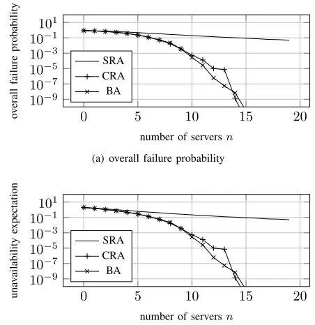
We first compare the algorithms proposed in Section V. For the ease of presentation we define the overall failure prob-ability as the probability that at least one function cannot be recovered, i.e., the overall failure probability equals one minus the survival probability. Likewise, we consider in this section

0 5 10 15 20

101

10−1

10−3

10−5

10−7

10−9

number of serversn

o

v

erall

failure

probability

SRA CRA BA

(a) overall failure probability

0 5 10 15 20

101

10−1

10−3

10−5

10−7

10−9

number of serversn

una

v

ailability

expectation

SRA CRA BA

(b) overall expected number of unavailable functions

Fig. 5. Performance comparison of the algorithms presented in Section V with

c= 4andk= 20.

0 5 10 15 20

101

10−1

10−3

10−5

10−7

10−9

number of serversn

o

v

erall

failure

probability

SRA CRA BA

(a) overall failure probability

0 5 10 15 20

101

10−1

10−3

10−5

10−7

10−9

number of serversn

una

v

ailability

expectation

SRA CRA BA

(b) overall expected number of unavailable functions

Fig. 6. Performance comparison of the algorithms presented in Section V with

c= 5andk= 20.

the unavailability expectation defined as the expected number of unavailable functions. Since both new definitions complement the original ones, our goal is to minimize those quantities.

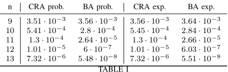
n CRA prob. BA prob. CRA exp. BA exp.

9 3.51·10−3 _3.56·10−3 _3.56·10−3 _3.64·10−3

10 5.41·10−4 _2.8·10−4 _5.45·10−4 _2.84·10−4

11 1.3·10−4 _2.64·10−5 _1.3·10−4 _2.66·10−5

12 1.01·10−5 _6·10−7 _1.01·10−5 _6.03·10−7

13 7.32·10−6 _5.48·10−8 _7.32·10−6 _5.51·10−8 TABLE I

COMPARISON OFCRAANDBAFORc= 4. THE TABLE SHOWS THE OVERALL FAILURE PROBABILITY(PROB.)AND THE UNAVAILABILITY EXPECTATION(EXP.)

n CRA prob. BA prob. CRA exp. BA exp.

7 1.18·10−2 _5.59·10−3 _5.41·10−2 _5.6·10−2

8 2.69·10−3 _8.68·10−4 _1.67·10−2 _2.3·10−2

9 4.48·10−4 _5.5·10−5 _3.56·10−3 _3.64·10−3

10 5.46·10−5 _6.69·10−6 _5.45·10−4 _2.84·10−4

11 1.72·10−5 _7.85·10−7 _1.3·10−4 _2.66·10−5 TABLE II

COMPARISON OFCRAANDBAFORc= 5. THE TABLE SHOWS THE OVERALL FAILURE PROBABILITY(PROB.)AND THE UNAVAILABILITY EXPECTATION(EXP.)

on average case analysis. Hence, for each n ∈ {0,1, . . . , k−1}, we created 500 random instances of failure probabilities vectors, where each failure probability is uniformly distributed over the range[0.025,0.175]. This range was selected by the considerations presented in Section VI-C.

As depicted in Fig. 5 and Fig. 6, the CRA and the BA algorithms outperform the SRA algorithm for all values ofn. While their per-formance seems similar for small values ofn, the CRA algorithm is slightly better than the BA algorithm in this case. This is due to the fact that the BA algorithm balances the connected component probability based on their failure probabilities product, which is suitable for c = 2, while the CRA algorithm basically assigns backups to the functions with the top mostc·nfailure probabilities (for k ≥c·n). However, this range of values for the number of serversnis not of much interest since it typically results in too high overall failure probability and unavailability expectation. Note that if one is interested in extremely low overall failure probability (and unavailability expectation), then the CRA algorithm shows better results also for this case, where the number of servers is large.

Note also the similarity between the results for the two problems, both in Fig. 5 and in Fig. 6 (between the two sub-figures in each figure). This demonstrates the extreme similarity of the two problems, as discussed in Section IV-C.

Table I and Table II 1 _{distinguish between the overall failure} probability and unavailability expectation of the CRA and BA algorithms for interesting values of n, when the overall failure probability and unavailability expectation obtained values are rea-sonable. The BA algorithm shows better results for all such values of n. As can be seen in the two parts of the tables, this is true for both problems.

Moreover, Tables III and IV show the standard deviation of the overall failure probability. The quality of the BA algorithm is demonstrated in a two-folded way. First, it shows better results for all (reasonable) values ofn. Second, as Tables III and IV show,

1_{For the journal version of this paper, we re-ran our simulations, increasing the}

number of instances, and fixed some minor bugs in the computer program. These modifications only slightly change the results reported in the conference version experiment section, where none of these changes is significant.

n CRA prob. std BA prob. std

9 2.5·10−3 _1.69·10−3

10 1.28·10−3 _1.59·10−4

11 6.39·10−4 _1.89·10−5

12 6.35·10−5 _5.58·10−7

13 1.16·10−4 _1.26·10−7 TABLE III

STANDARD DEVIATION OF THE SURVIVAL PROBABILITYPWITHc= 4

n CRA prob. std BA prob. std

7 5.7·10−3 _2.63·10−3

8 3.31·10−3 _4.54·10−4

9 1.62·10−3 _4.28·10−5

10 4.06·10−4 _5.86·10−6

11 3.33·10−4 _7.56·10−7 TABLE IV

STANDARD DEVIATION OF THE SURVIVAL PROBABILITYPWITHc= 5

2 3 4 5 6 7 8

6 8 10 12 14 16 18

number of backups per server (c)

number

of

serv

ers

(n) _CRA

BA

(a)Pd= 0.999

2 3 4 5 6 7 8

8 10 12 14 16 18

number of backups per server (c)

number

of

serv

ers

(n)

CRA BA

(b)Pd= 0.9999

Fig. 7. Number of servers needed to obtain a desired survival probabilityPdas a function ofc, withk= 20functions.

the CRA algorithm encounters a relatively higher standard deviation in results. A low-standard deviation in results is crucial when the number of functions is large and it may be hard to evaluate the exact survival probability and expectation, as discussed in Section VI-B.

B. Effect of the number of backups per server

We now examine the effect of the number of backups per server

c. Fig. 7 shows the number of servers required in order to achieve a survival probability of 0.999 and 0.9999 as a function of the number of backups per server,c, wherek= 20. We used the CRA and BA algorithms which showed best results, and ran our simulations for each c and k with 500 random instances of failure probabilities vectors, distributed as in Section VII-A.

For example, Fig. 7 demonstrates that for 20 functions (i.e.

CRA, or only approximately 10 servers using BA. If each server can have 5 backups then we can save one server for each case, resulting in approximately 10 and 9 servers, respectively. From Fig. 7, we can conclude that most of the improvement in the number of required servers is achieved forc= 4,5which justifies the selection of these values in the rest of the simulations.

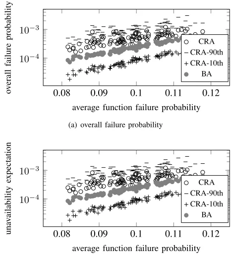
C. Between CRA and BA

In section VII-A we showed that while the BA algorithm only slightly improves upon the CRA algorithm, CRA shows large variance compared to BA. In this section we show that the large variance of CRA can be exploited in cases where theexactoverall survival probabilities and the unavailability expectation can be computed, i.e., where the number of functions is small.

Fig. 8(a) and Fig. 8(b) show statistics of the overall failure probability and the unavailability expectation as a function of the average function failure probability. We setk= 20,c= 4,n= 10, and created 100 random instances of failure probabilities vectors, where each failure probability is uniformly distributed over the range[0.025,0.175](as in Section VII-A). For each such vector, we ran 100 times the CRA algorithm, gathering its 10th percentile, 90th percentile, and its mean (for both the overall survival probability, and the unavailability expectation), then we ran BA once. Since BA is a deterministic algorithm, no statistics gathering required (or possible). Note that Fig. 8(a) and Fig. 8(b) show the complement of the above quantities, that is, the overall failure probability and the unavailability expectation. Therefore, the 10-th percentile appears lower than the 90-th percentile.

As both Fig. 8(a) and Fig. 8(b) show, if the number of functions is low so that exact overall survival probability and unavailability expectation can be computed, one may run the CRA algorithm multiple times, saving the construction at each time, and then taking the construction which led to the best results. This process makes CRA perform better than BA. However, when the number of functions is larger, assuming that the difference between CRA mean performance and BA performance is also valid, BA should be favored.

D. Post Failure Recovery Probability

In this section we consider a scenario where the failures of the functions occur in two phases. In the first phase some functions fail and then recovered, that is, specific servers are used to recover the functions, where the assignment of function backups to other servers is unchanged. Then, in the second phase, other functions may fail. These functions can be recovered only by servers that were not used for recovery in the first phase.

Fig. 9(a) and Fig. 9(b) show the overall failure probability and the unavailability expectation at the start of the second phase (that is, after the first-phase failure and recovery), as a function of the number of functions that fail in the first phase. As in previous subsections, we set k = 20, c = 4, n = 10, and created 500 random instances of failure probabilities vectors, where each failure probability is uniformly distributed over the range [0.025,0.175]. For each such vector and for each q ∈ {0, . . . ,5}, we picked q

functions uniformly at random, considered them as the first phase failing functions and recovered them using servers according to the specific assignments retrieved by CRA and BA. Then, we

0.08 0.09 0.1 0.11 0.12

10−4

10−3

average function failure probability

o

v

erall

failure

probability _CRA

CRA-90th CRA-10th

BA

(a) overall failure probability

0.08 0.09 0.1 0.11 0.12

10−4

10−3

average function failure probability

una

v

ailability

expectation _CRA

CRA-90th CRA-10th

BA

(b) overall expected number of unavailable functions

Fig. 8. Performance comparison of the CRA and BA algorithms withc= 4and

n= 10andk= 20.

determined the overall failure probability and the unavailability expectation in each of the assignments (when disregarding the q

picked functions and theqcorresponding servers used for recovery). As both Fig. 9(a) and Fig. 9(b) show, the overall failure prob-ability and the unavailprob-ability expectation in the second phase gets significantly larger when the number of functions that fail in the first phase increases. For instance, while for both CRA and BA the overall failure probability and the unavailability expectation is below10−3, forq= 3the corresponding values are approximately 0.1.

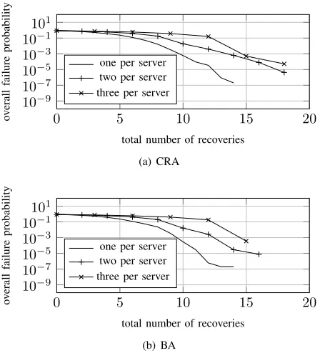
E. Servers Recovering Multiple Functions

Until this point we focused on the case where each server is capable of recovering exactly one function upon its failure, here we consider the case where each server is capable of recovering up to r functions. In this case, we basically use the exact same solutions proposed for the single recovery per server case.

Fig. 10(a) and Fig 10(b) show, for both CRA and BA, respec-tively, the overall failure probability as the function of total number of recoveries the system is capable of, that is, the number of servers multiplied by the number of recoveries per server n·r. We set k= 20functions, and for each n∈ {0,1, . . . , k−1}, we created 500 random instances of failure probabilities vectors, where each failure probability is uniformly distributed over the range

[0.025,0.175]. Then for each such vector we applied CRA and BA and determined their overall failure probability for r ∈ {1,2,3}