The Effect of Zimbabwe’s Multi-Currency Arrangement on Bilateral Trade: Myth versus Reality.

Issues

ISSN: 2146-4138

available at http: www.econjournals.com

International Journal of Economics and Financial Issues, 2015, 5(3), 690-700.

The Effect of Zimbabwe’s Multi-Currency Arrangement on

Bilateral Trade: Myth Versus Reality

Steven Buigut*

School of Business, American University in Dubai, Dubai, UAE. *Email: [email protected]

ABSTRACT

To tame the hyperinflation experienced in the country, Zimbabwe adopted a relatively unique solution by implementing a multi-currency system in January 2009. Five foreign currencies were granted official status. However, this arrangement is viewed as a temporary measure to restore stability

and there is no commitment by authorities to maintain it long-term. The present study uses a theoretically consistent gravity model that accounts for

endogeneity, to estimate the effect of the multi-currency arrangement implemented in Zimbabwe on bilateral trade. The period covered by the study is from 2004 to 2012 using a total of 50 potential trading partners from Africa, Asia, Western Europe, Eastern Europe, North and South America. The results suggest that the multi-currency arrangement as adopted has depressed Zimbabwe’s bilateral trade by nearly 15%.

Keywords: Multi-Currency Regime, Gravity Model, Trade, Zimbabwe

JEL Classifications: F14, F15, F33

1. INTRODUCTION

To tame the devastating hyperinflation, Zimbabwe introduced a multi-currency regime in January 2009. Unlike in traditional

dollarization schemes where a dollarizing country adopts one hard

currency, five currencies initially were legally allowed to circulate

at the same time. The currencies adopted initially are the US dollar, Euro, UK Sterling pound, South African Rand and Botswana Pula. Further, there is no long-term commitment to this regime

by authorities in Zimbabwe. The adoption of the multi-currency

regime is viewed as a temporary measure to restore stability, and

even the number of currencies included in the basket is mutable. In

early 2014, this basket of currencies was expanded to include four

new currencies, namely the Australian Dollar, Chinese Yuan, Indian

Rupee, and Japanese Yen (Reserve Bank of Zimbabwe, 2014). It is expected that at some point the multi-currency arrangement will be abandoned. But there is as yet no official time line or indication what new monetary regime will replace it. The lack of an immediate plan to change has not eliminated market jitters though.1

1 After rumors started circulating, the governor of the Reserve Bank of Zimbabwe on 6th _{August 2013, issued a statement to reassure the market} that there were no plans to re-introduce the Zimbabwe dollar in the immediate or near term (Gono, 2013).

Credibility will be a major concern in the choice of a monetary

policy framework to replace the multi-currency regime given the culpability of the Reserve Bank of Zimbabwe (RBZ) in the recent hyperinflation. Kramarenko et al. (2010) review the pros and cons of alternative monetary regimes available to Zimbabwe to succeed the multi-currency system. They opine that some form of official dollarization rather than a rush to re-introduce the Zimbabwean

dollar as sole currency would be preferable. The two leading options they propose are membership in the common monetary

area (CMA)2_{, and official dollarization with the US dollar as sole}

legal tender.

Since the introduction of the multi-currency regime in 2009, output and trade in Zimbabwe has slowly recovered. The present study takes advantage of this rare event experienced in Zimbabwe

to provide evidence of the effect of a multi-currency regime on

bilateral trade. To the best of our knowledge this is the first study to attempt to answer this question. A large literature has assessed the effect of currency union (dollarization) on bilateral trade. A smaller list of researchers (e.g. Klein and Shambaugh, 2006; Adam and Cobham, 2007) have investigated an expanded menu of exchange

rate regimes. This paper attempts to extend this strand of literature to the use of multiple currencies. We present a quick overview of the causes of the Zimbabwe hyperinflation before discussing the literature on exchange rate regimes and trade.

1.1. The Genesis of Hyperinflation and the Original

Sin

Various forces have been blamed for fueling Zimbabwe’s hyperinflation, ranging from socio economic factors and political instability to military adventurism. Critical also was the lack of independence of the RBZ. The start of the decline can be traced back to 1997. However, one of the basic ingredients was actually inherited at birth. When Zimbabwe attained political independence in 1980, she inherited a highly skewed land distribution. Some 4500 large scale commercial farms covering about 11 million hectares (ha) of the best arable land were owned largely by white farmers (AfDB/OECD, 2003). In contrast, about 1.2 million indigenous households (about 40-50% of the total population then) subsisted on 16.6 million ha of poorer quality, drought prone land.

In an effort to redress the problem, the government resettled over

3 million ha under the “first option to buy” conducted at market prices (Coomer and Gstraunthaler, 2011; IMF, 2001) during the first half of 1980’s. This process however slowed down during

the second half of the period. The 1992 land act provided for compulsory purchase of farms, as long as the property was derelict, located on underutilized land, owned by absentee landlord, or surrounded by communal areas, and the owner had multiple farms

(IMF, 2001). The act required fair compensation and provided for right of appeal. However the new act did not add much traction to

the pace of resettlement. But it paved the way for the government

to ratchet up the process in subsequent years.

To deflect the growing despondency among war veterans the government in August 1997 awarded a new compensation and monthly pension to approximately 60,000 war veterans (Coomer and Gstraunthaler, 2011; Kairiza, 2009) the value of which amounted to about 3% of gross domestic product (GDP) at the time. The award, approximately USD 3000 immediate

payment at the time and 125 USD monthly payment, served to

increase the budget deficit as it was not properly budgeted for. And in November 1997 President Mugabe announced plans for the compulsory acquisition of white-owned farms. About 1,471 commercial farms were gazette for compulsory acquisition (Coomer and Gstraunthaler, 2011; Kairiza, 2009; IMF, 2001). Without a clear indication of how this was to be financed, the plan spooked investors and strained relations with the World Bank (WB) and International Monetary Fund (IMF). Informal land invasion and the launch of the fast-track development programme covering 5 million ha and 150,000 families in mid-2000 increased

uncertainty and had a major impact on agricultural production.

Military adventurism also contributed to the fiscal burden. In

September 1998 President Mugabe send troops to the Democratic Republic of Congo to support the beleaguered President Laurent

Kabila. Kairiza (2009) estimates the cost to Zimbabwe could

have been in the range of USD 1.3 billion per month in 1998.

As Zimbabwe experienced these events that swelled the fiscal

burden, a mismanaged land reform spawned uncertainty and

shrunk production. With the donors limiting and withdrawing support, the RBZ found itself saddled with the task of supporting the fiscal operations.

The journey to hyperinflation and the eventual demise of the Zimbabwe dollar have been well chronicled in a number of studies (for example Hanke and Kwok, 2009; Hanke, 2012; Coomer and Gstraunthaler, 2011; Kairiza, 2009; Coltart, 2008; Noko, 2011; Ndlela, 2011). Crucially, the RBZ’s lack of independence and its inability to contain the quasi-fiscal role thrust upon it hampered efforts to contain the hyperinflation. The result was the second highest inflation in history according to estimates by Hanke and Kwok (2009) who have attempted to construct a more complete record of Zimbabwe’s inflation beyond July 2008 when the official inflation data ceased. Their computations suggest that the highest monthly inflation rates occurred in mid-November 2008 and reached month-over-month rate of 79.6 billion percent. Their estimated year-over-year rate is a staggering 89.7 × 1021 _percent.

Faced with a hyperinflation of this magnitude, the market basically rejected the Zimbabwe dollar, and de facto dollarization ensued. Bowing to reality the RBZ, toward the end of September 2008, introduced what it called foreign exchange licensed warehouses and shops (FOLIWARS), initially intended for a trial period

of 18 months to March 31st_{, 2010 (Gono, 2008). A number of}

retail and wholesale outlets were licensed as foreign currency denominated shops, to sell goods and services in foreign currency. Under this program, only the licensed outlets were legally authorized to charge in foreign currency. In addition there was

a rather long list of basic commodities that were required to be payable in the local currency even in the FOLIWARS. Shops not licensed under FOLIWARS, along with critical service providers such as commuter transporters, were required to charge in local

currency.

1.2. The Era of Multi-Currency Regime

The Zimbabwe hyperinflation ended with the introduction of

the multi-currency system. This also spelt the demise of the

Zimbabwean dollar. The currency reforms contained in the monetary policy statement of January 2009 (Reserve Bank of Zimbabwe, 2009) allowed for the circulation of multiple currencies in the economy and sought to close the RBZ’s quasi-fiscal operations.

As Zimbabwe struggles with restoration it is appropriate at this point to take stock of the impact this regime has had on the country’s economy. By adopting a multi-currency regime the RZB effectively gave up its monetary policy as a policy tool to influence the economy. However an obvious benefit of the

multi-currency regime is price stability. Since the introduction of the

multiple currency regime, the rampant inflation has been tamed.

Figure 1 shows inflation rate has declined to settle at around 3%. Economic growth has shown signs of picking up though the

recovery is still fragile.

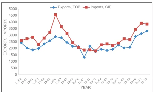
about 50% to a low of 4.41 billion US dollars in 2008. After 2008, it has risen by about 33% to 5.88 billion in 2012. In per capita terms the GDP declined 50% from 718.4 constant (2005) US dollars in 1998 to 344.7 US dollars in 2008. Since then it has recovered about 24% to 428.5 US dollars in 2012. The value of exports (Figure 3) shows a decline from 1996 and remains depressed through 2009. The worst export performance was recorded in the year 2001 coinciding with the escalation of land reforms under the fast-track development programme. Imports depict a similar trend. Both imports and exports show some recovery after 2009.

2. EXCHANGE RATE REGIMES AND

BILATERAL TRADE

There is a large literature attempting to estimate the effect of a

common currency on trade. Rose’s seminal work (Rose, 2000) as well as subsequent work with co-authors (such as Frankel and Rose, 2002; Glick and Rose, 2002; Rose and van Wincoop, 2001)

use a gravity model to investigate the effect of currency union on bilateral trade. The large size of the impact they obtained (about

3 times in Rose, 2000) generated a wave of research, much of it attempting to “shrink” this effect in the vein of Nitsch (2002). Rose and Stanley (2005) perform a meta-analysis (of about 34 studies) of the currency union effect and suggest a range of 30-90% as the

currency union effect. More recent studies shave this effect even more. The consensus now seems to be that currency union does have some positive impact on bilateral trade but way less than

originally predicted by Rose (Baldwin, 2006). For example recent

estimates put the effect of the Euro on bilateral trade in the single

digits (Bun and Klaassen, 2007; de Nardis et al., 2008). Jagelka (2013) also estimates a Euro effect of about 9% on bilateral trade

of the newest Eurozone members (Slovenia, Malta, Cyprus, and

Slovakia) who joined between 2007 and 2009.

Some studies (e.g. Tsangarides et al., 2008; Qureshi and Tsangarides, 2011) have found that currency union effect of African currency unions is significantly positive and not much different from other estimates of the rest of the world. However,

using a model of the welfare implications of forming a currency

union, Masson (2008); Debrun et al. (2005) show that the effects

from forming a currency union in Africa depends very much on the membership of that union. Asymmetries across countries would

make even regional currencies undesirable for some countries. Buigut and Valev (2009) using a closely related model calibrated

for the east African community shows support for these results.

These studies however have focused on the traditional monetary union such as Euro, or the adoption of one hard currency (such

as the US dollar) by a country as legal tender in the simple

form of dollarization. Some researchers however have tried

to expand the menu of exchange rate regimes considered. For example Klein and Shambaugh (2006) extend the analysis to fixed exchange rates. They find a positive and significant effect of a fixed exchange rate regime on bilateral trade. Adam and Cobham (2007), using a theoretical gravity model suggested by Anderson and van Wincoop (2003; 2004), attempt to identify the effect on trade of a wide range of bilateral exchange rate regimes including currency union, pegging, managed floats and full floats. They find that some regimes other than currency union are also significantly pro-trade than flexible exchange rates. In summary, they find that there is a gradual positive effect on trade as uncertainty and transaction costs are reduced. Qureshi and Tsangarides (2011) suggests that both currency unions and

direct pegs promote bilateral trade in Africa relative to more

flexible exchange rates.

The present paper extends this strand of literature to multi-currency regimes as adopted in Zimbabwe. Several aspects of this

regime differentiate it from what has generally been the focus of -6.0

-4.0 -2.0 0.0 2.0 4.0 6.0 8.0

Jan-10 Mar-1

0

May-1

0

Jul-10 _{Sep-10 Nov-1}

0

Jan-11 Mar-1

1

May-1

1

Jul-11 _{Sep-11 Nov-1}

1

Jan-12 Mar-1

2

May-1

2

Jul-12 _{Sep-12 Nov-1}

2

Jan-13 Mar-1

3

May-1

3

Jul-13 _{Sep-13 Nov-1}

3

Year on Year Price Increas

e

Figure 1: Zimbabwe’s year on year inflation, 2010-2013

Source: Reserve Bank of Zimbabwe, http://www.rbz.co.zw

0 1E+09 2E+09 3E+09 4E+09 5E+09 6E+09 7E+09 8E+09 9E+09 1E+10

1990 1991 1992 1993 1994 1995 1996 1997 1998 1999 2000 2001 2002 2003 2004 2005 2006 2007 2008 2009 2010 2011 2012 2013

GDP

Years

Figure 2: Gross domestic product constant (2005) US dollars, 1990-2012

Source: The World Development Indicators, April 2014

0 500 1000 1500 2000 2500 3000 3500 4000 4500 5000

EXPORTS, IMPORT

S

YEAR Exports, FOB Imports, CIF

Figure 3: Export and import values (millions of 2005 US dollars), 1990-2012

existing literature, making this study a worthwhile pursuit. First, the adoption of several currencies at the same time is unique. Usually a dollarizing country would pick one currency to adopt. Zimbabwe adopted five currencies at once, and in 2014 has added another four. The benefits of sharing a single currency generally

cited include reduction of transaction costs related to trade. It also helps enhance transparency, and provide a credible commitment to

exchange rate stability. However in the case of a multiple currency regime, these benefits may not be forthcoming. The use of multiple currencies is likely to cause confusion and reduce clarity that is so essential in market transactions. For example a firm in Zimbabwe which decides to operate using “Euros” because its major market is in the “Eurozone” for example, would still have to interact with other firms/agents locally that may have opted to use the “Rand” or any of the other three currencies. Hence economic

agents face added transaction costs internally. Technically, the

Zimbabwe economy is subdivided into five, albeit unequal and overlapping common currency (dollarized) zones. Such

sub-divisions and overlaps lead to transactional inconvenience and

related transaction costs. Noko (2011), explaining the experience in Zimbabwe, states that Rand/US dollar exchange rates differ

from city to city and even from shop to shop within a city. The

increased dominance of the US dollar is then partly explained

as a shift towards transactional convenience and the importance of the state in the economy which carry out budget estimates in

dollars and pay most civil service wages in dollars (Kramarenko et al., 2010; Noko, 2011). Some estimates suggest that around 80% of the transactions take place in dollars (Kramarenko et al., 2010). The transactional inconvenience is a shortcoming of

the use of multiple currencies. There is a second shortcoming

related to how it was implemented in Zimbabwe. There is no

long-term commitment to the multi-currency arrangement by the

authorities in Zimbabwe. It is not clear how long it will last and there is currently no framework explicitly laying out a structure

for the replacement of the regime. This certainly is a source of

uncertainty for the market.

The interesting question posed in this study then is “would

a temporary dollarization arrangement that uses multiple

currencies have any effect on bilateral trade?” This question, to the best of my knowledge, has not been directly answered before, and forms the focus of the present study. The Zimbabwean experience provides a unique experiment that could shade some

light on it.

The rest of the paper is organized as follows: Section 3 briefly

reviews the gravity model, Section 4 and 5 describe the data and empirical model respectively. In Section 6 the results are discussed

and concluding remarks provided in Section 7.

3. THE GRAVITY EQUATION

Basically, the gravity equation relates trade between two countries to GDP, distance, and other variables that influence

trade. The effects of a monetary union/free trade agreement

(FTA) is then measured by a currency union/FTA dummy.

A traditional gravity model commonly estimated using cross

section data takes the form:

ln ln ln ln

ln

X d Y Y

CU Z

ij ij i j

ij n ij

  = +   +

[ ]

+ +

β β β

β α

0 1 2 3

4 nn

n=1 N

ij

∑

(1)

Where ln Xij are the natural logs of exports from country i to j, dij

is the distance between countries i and j, Yi and Yj are the GDP

of exporter and importer (source and destination) countries, (n = 1…N) a set of other observables which influence bilateral trade. CU is a binary variable taking the value of one if i and j share

a currency and zero otherwise, while εij is assumed to be a

log-normally distributed error term.

Increasingly, however, studies have cautioned against the use of the

traditional, atheoretical, gravity model as shown in Equation (1).

These studies suggest that countries select endogenously into monetary unions or FTAs for a host of reasons that may include historical, cultural, and other unobservable reasons that are

likely to be correlated to level of trade. Hence the estimation of the effects of currency union (or FTAs) on trade is plagued with endogeneity issues. Magee (2003) shows that higher bilateral trade flows increase the likelihood that countries will form FTAs.

In their study of the economic determinants of FTAs, Baier and

Bergstrand (2004) find strong evidence that countries that have

FTAs tend to share economic characteristics that should enhance

net economic welfare gains from an FTA. For example countries

tend to have an FTA the larger and more similar their GDPs, the closer to each other, and the more remote the country pair is from

the rest of the world. These variables also tend to explain a large amount of trade flows between countries.

The switch to multi-currency in Zimbabwe was not planned, but still the choice of the five currencies introduced in 2009 can be linked to trade. South Africa is Zimbabwe’s leading trading partner,

followed by the European Union. The US is a major source of

imports. The acting Governor of the RBZ (Dr. Dhliwayo) cited

increasing trade and investment with the respective countries as

reason for the choice of the new currencies added to the basket of circulating currencies in 2014 (Reserve Bank of Zimbabwe, 2014).3 _{Thus the endogeneity problem would still be a factor to}

consider.

First used by Tinbergen (1962), earlier applications of the gravity

model where not grounded in a formal theoretical foundation. After

the initial attempt by Anderson (1979), a number of studies have

contributed to the development of the theoretical foundation of the

empirical gravity equations. Some recent key works to contribute to the development of the theoretical foundation of the gravity equation include Feenstra (2002); Feenstra (2004); Anderson and van Wincoop (2003); Anderson and van Wincoop (2004). The theoretical gravity equation suggests the need to account for multilateral price variables – termed “multilateral resistance” in the literature.

Anderson and van Wincoop (2003) show that starting from identical homothetic preferences approximated by a constant elasticity of

3 The unplanned nature of the multi-currency regime introduced in Zimbabwe

substitution utility function, with all goods differentiated by place

of origin, the gravity equation can be presented as:

X YY Y t P ij i j w ij i j =             − Π 1σ (2)

Πi ij j

j j =     

∑

t P 1

1 1

σ σ

θ

(3)

Pj tij i

i i =    

∑

Where, Y_w is the world GDP, t_ij the trade cost factor (bilateral trade

barriers) between i and j. The σ is the elasticity of substitution

between all goods, with θi i w

≡ 

 YY  and θj j w ≡     Y

Y the income

shares, while Pj is countryj’s overall price index defined as in

Equation (4). Anderson and van Wincoop then assume symmetric

trade barriers (t_ij = t_ji) to show that a solution for Equations (3) and (4) is Πi =Piwith:

Pj1- t Pij i j

i i

σ ₌

∑

(5)

The gravity equation then becomes:

X YY Y t PP ij i j w ij i j =             − 1σ (6)

Equation (6) suggests that the bilateral trade between countries

depends on their GDPs and also on their implicit price indices.

Anderson and van Wincoop call the price indices P_i “multilateral

resistance” variables because they depend on all bilateral resistance

(tij). They then model the unobservable trade cost factor tij as a

log linear function of observables, bilateral distance (dij) and

whether there is an international border (b_ij) between i and j as

in Equation (7). Note however, that the list of observables used in the trade cost function is often extended in the literature to

include directly measured trade costs, adjacency, preferential trade membership and common language among others.

tij=b dij ijρ ₍₇₎

Taking logs in Equation (2), and substituting Equation (7) for transport costs, Anderson and van Wincoop provide the theoretical

gravity model:

ln ln ln ( ) ln ( )ln

( )ln ( )ln

X k Y Y d b

P

ij i j ij ij

i

= + + + − + −

− − − −

1 1

1 1

σ ρ σ

σ σ PPj ₍₈₎

The main difference between the traditional gravity model

in Equation (1) and the theoretical gravity equation shown in

Equation (8) is the multilateral resistance terms. Since these terms

are correlated with distance and border effects, they create an omitted variable bias if not accounted for.

The literature proposes three different approaches to estimating

this theoretical gravity equation. Briefly, the first approach

is to use multi-country price indices and apply ordinary least

squares (OLS) (e.g. as in Baier and Bergstrand, 2001). The

shortcoming of this approach is that published price indices may

not accurately reflect the true border effects (Feenstra, 2002). The second approach is to use non-linear least squares as adopted in Anderson and van Wincoop (2003). Though it produces consistent estimates, this approach requires custom programing to perform the constrained minimization. A third technique is to replace the

multilateral resistance indices with inward and outward

region-specific (importer and exporter) dummies. Examples of studies that apply this approach are Hayakawa and Yamashita (2011); Feenstra (2002); Baier and Bergstrand (2007). Like the second

approach the third approach also produces consistent estimates. For a more detailed discussion of these approaches see for

example Anderson and van Wincoop (2004); Feenstra (2002); Hayakawa and Yamashita (2011). This paper follows the third

approach and include country-and-time effects as in Baier and

Bergstrand (2007).

Baldwin (2006); Baldwin and Taglioni (2007) identify three

common errors they dub the gold, silver and bronze medal errors

in the gravity equation estimation. The gold medal error is related

to the endogeneity just discussed above. The silver medal error,

they content, is the most common mistake researchers make. Gravity equation explains uni-directional bilateral trade. Most researchers estimate the gravity equation using the average of the two-way exports (average of Country A exports to Country B, and Country B exports to Country A) rather than uni-directional flows (e.g., exports of Country A to Country B). The mistake is

in how the averaging is done. The correct way, they point out,

is to take the average of the sum of logs of the two trade flows,

not the log of the average. The bronze medal error is related to

the deflation of the nominal trade data using US aggregate price index. This, they suggest causes bias since there are global trends in inflation rates.

This study estimates the bilateral trade effects of Zimbabwe’s

multicurrency regime using a theoretically founded panel

gravity equation and attempts to account for the source of bias. Country-pair fixed effects (ij) are included to control for

historical and time constant factors that affect the level of trade between partner countries. In addition, to account for time varying multilateral resistance, country-and-time (both source

and destination) (it, jt) effects are included. Country-and-time fixed effects capture the changes in output, income per capita,

population and other variables that are included in a gravity

specification. Further, as Magee (2008) notes, fixed effects are more flexible as they also capture any aggregate shocks to the countries’ trade flows in a given year. This eliminates the

4. DATA SOURCES

Uni-direction trade data is obtained from the IMF’s Direction of Trade Statistics (May, 2014) in nominal US dollars. The period considered is for the years 2004-2012 with a total of 50 potential trading partners. Thus only the first five currencies introduced 2009 are considered, not the second set of currencies introduced in 2014. The end period is dictated by the availability of data. The countries included cover Africa, Asia, Western Europe, Eastern Europe, North and South America and are listed in the Appendix.

As suggested by Baldwin and Taglioni (2007) uni-directional trade is used. However, averaged data is used for robustness checks. With 50 countries and 9 years there are 44,100 (2 × N × N−1 × T) bilateral trade data points, since each trade flow is reported as import and export. Of these there were 183 and 27 zero and missing respectively. In line with a number of studies (e.g., Carrère, 2006; Magee, 2008) only non-zero values are included in the analysis. When the missing or zero import values are excluded we have 43,890 observations

left in the analysis. Botswana, one of the countries whose currency was adopted is not included due to incomplete data. One half of the trade records is unavailable.4 _{The key control variables included are}

the GDPs sourced from the WB’s World Development Indicators (April, 2014). Other variables that may influence trade flows such as

distance between trade partners, contiguity, similarity in languages, and colonial relations are sourced from the Institute of Research on

International Economy (CEPII) data base.5

5. EMPIRICAL MODEL

Our primary interest is to identify the average effect on bilateral trade arising from the adoption of the of multi-currency regime in

Zimbabwe. The theoretical gravity model discussed in Section 3

recommends the inclusion of multilateral resistance terms. In a panel format this suggests the following:

ln

X

ln[

gdp

]

ln

distcap

contig

ijt

ijt

ij

ij

=

+

+

+

 

 _

 

 

β

β

β

β

0

1

2

4

+

+

+

+

−

β

β

β

β

5

6

7

45

comlang

comcol

col

mcu

P

ij

ij

ij

mcu

ijt

[

]

ln iit

1

− −

σ

ln

P

jt

1

− +

σ ε

ijt

(9)

Where ln is the natural logs. mcuijt is a dummy variable to capture

the multi-currency system. A significant βmcu>0 coefficient would

imply that the use of multiple currencies has had positive effect on

Zimbabwe’s bilateral trade. Several other variables are included.

The variables included (contig, comlang, comcol, col45, distcap,

gdp and mcu) and their expected signs are described in Table 1. 4 Botswana’s export/ import data, as reported by Botswana, is missing in the

Direction of Trade Statistics (DOTS). It is only available as reported by trade partner countries as imports/exports respectively. Since our approach uses uni-directional trade data (not averaged data) as the dependent variable, we decided to exclude this country.

5 These are sourced from http://www.cepii.fr/anglaisgraph/bdd/distances.

htm. (dist_cepii.xls file)

Including the country-pair fixed effects (ij), such thatα_ij ≠α_ji , accounts for the impact of distance between countries, common language, adjacency, colonial status or other historical ties and other unobserved characteristics of the country pair that are

constant over time. Therefore with these bilateral fixed effects included, the equation estimated is:

lnXijt =β α0+ ij+β1lngdpijt+βmcumcuijt+εijt ₍₁₀₎

Note that in a panel setting the multilateral resistance variables

would be time-varying. Hence using only bilateral fixed effects,

(ij) may result in omitted variable bias.

Including exporter-year and importer-year, that is

country-and-time for both source and destination, effects (it, jt) will account

for variations in GDPs, population, multilateral resistance terms

and other unobserved time-specific shocks. The estimated equation

will in effect be:

lnXijt =β α0+ ij+αit+αjt+βmcumcuijt+εijt ₍₁₁₎

A major advantage of (11) is that it controls for nearly every variable included in gravity equation and unobserved factors. It thus tempers the difficult choice about which of the many variables one needs to include in the model. The main disadvantage of (11)

is that it is not possible to estimate the effect of any other factors that affect bilateral trade even if time varying.

6. RESULTS

To get an initial sense of the effect of the multi-currency

arrangement, a traditional gravity equation (pooled OLS) is estimated. This is obtained from estimating Equation (9) excluding bilateral fixed effects, and ignoring the multilateral resistance

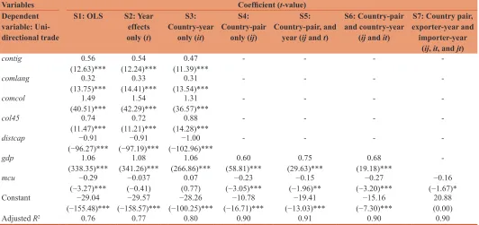
terms. The results are shown in Table 2 as specification 1 (S1). The

dependent variable is the natural log of uni-directional bilateral trade. The control variables included (contig, comlang, comcol,

col45, distcap, and gdp) all are significant and carry the expected sign. Of special interest is the coefficient on multi-currency

variable (β_mcu). This is negative (−0.29) and significant at 1%

level, suggesting that the adoption of multicurrency regime has

depressed bilateral trade by about 25% (100*[e−0.29_{−1] = 25.2%).}

This basic estimate, however, ignores the endogeneity issue

(baptized the “gold medal error” in Baldwin and Taglioni, 2007). Various specifications of the gravity model that attempt to account

for this are estimated. The results are shown in Table 2, columns

S2-S7. To control for historical and time constant factors that affect the level of trade between partner countries, country-pair fixed

effects (ij) are used as indicated in Equation (10). These control for characteristics that are time constant. Hence in addition to the mcu, only the gdp is included as the other variables are constant over time. The results are shown in Table 2 (S4). The coefficient

on gdp is the expected sign and significant. The coefficient on mcu

(β_mcu) reduces somewhat to −0.23 (a 20.5% decrease in bilateral trade). It is still significant at 1%. To account for both time-constant

and country-and-time (it and jt) (source and destination) fixed effects are included as in Equation (11). The result are provided

in Table 2 as S7. The coefficient on mcu is −0.16, and significant at 10%, indicating a negative impact of about 14.8% on bilateral trade. Other specifications are provided in Table 2. But we note

that all the specifications that include both (ij) and some form of time effects (S5-S7) show a negative value for the (βmcu) ranging

from 13.9% to 23.7%.

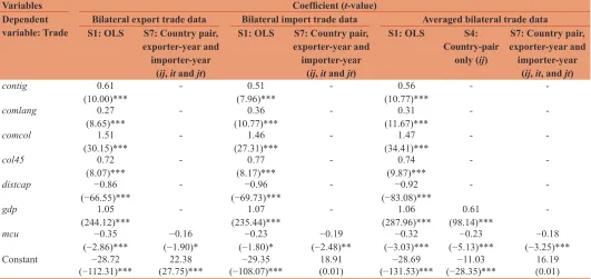
Table 3 provides some robustness checks. The mcu effect is

re-estimated, alternately using uni-directional exports (imports)

and averaged bilateral trade data as the dependent variable as

is the practice in several studies. The first two columns uses

uni-directional exports as the dependent variable, while the next

two columns imports is the dependent variable. For brevity only

specification results corresponding to S1 and S7 in Table 2 are provided. The results are similar to what was observed in Table 2. The mcu effect seen in S7 in Table 3 are −0.16 and −0.19 (14.8% and 17.3%). Note that the mcu effect in S7 in Table 2 was also

about 14.8%. The last three columns of Table 3 shows estimates Table 1: Definition of variable used in regressions

Variable Description (expected sign)

Bilateral trade: (Xijt) The dependent variable is nominal uni-directional bilateral data in US dollars. The natural log of

bilateral trade is used

Contiguity: (contig) A dummy variable equal one if the two countries (i and j) are contiguous, and zero otherwise (positive) Common language- official:

(comlang) A dummy variable equal one if the two countries share a common official language, and zero otherwise (positive)

Common colonizer _after

45: (comcol) A dummy variable equal one if the country pair were ever colonies and had a common colonizer after 1945, zero otherwise (positive)

Colonial relationship after

1945: (col45) A dummy variable equal one if the two countries have had a colonial relationship after 1945, zero otherwise (positive)

Distance: (distcap) Great circle distances calculated between capitals cities of country pair. The natural log of distance is

used (negative)

Product of the GDPs:

(gdpijt) The product of the nominal GDPs in US dollars (GDPvariable. The natural log of the product of the gdps of the country pair is used (positive)it*GDPjt) is used to represent the economic mass

Multi-currency

variable: (mcu) A dummy variable equal one if Zimbabwe is in a multi-currency arrangement with the trade partner since 2009, zero otherwise. To operationalize this, mcu=1 for countries whose currency Zimbabwe

adopted in 2009. These are US, South Africa, UK, and Euro countries.6 _{Also, mcu=1 for countries in a}

CB or conventional peg (P) arrangement with any of these four countries.7 _{The countries identified and}

included in the currency share arrangement with Zimbabwe are shown in the Appendix. (positive)

GDP: Gross domestic product, CB: Currency board

Table 2: Gravity equation estimates using uni-directional trade data

Variables Coefficient (t-value)

Dependent variable: Uni- directional trade

S1: OLS S2: Year effects only (t)

S3: Country-year

only (it)

S4: Country-pair

only (ij)

S5: Country-pair, and

year (ij and t)

S6: Country-pair and country-year

(ij and it)

S7: Country pair, exporter-year and importer-year

(ij, it, and jt)

contig 0.56

(12.63)*** (12.24)***0.54 (11.39)***0.47 - - -

-comlang 0.32

(13.75)*** (14.41)***0.33 (13.54)***0.31 - - -

-comcol 1.49

(40.51)*** (42.29)***1.54 (36.57)***1.31 - - -

-col45 0.74

(11.47)*** (11.21)***0.72 (14.28)***0.88 - - -

-distcap −0.91

(−96.27)*** (−97.19)***−0.91 (−102.96)***−1.00 - - -

-gdp 1.06

(338.35)*** (341.26)***1.08 (266.86)***1.06 (58.81)***0.60 (29.63)***0.75 (19.18)***0.68

-mcu −0.29

(−3.27)*** (−0.41)−0.037 (0.77)0.07 (−3.05)***−0.23 (−1.96)**−0.15 (−3.20)***−0.27 (−1.67)*−0.16

Constant −29.04

(−155.48)*** (−158.57)***−29.57 (−100.25)***−28.26 (−16.71)***−10.78 (−13.03)***−19.41 (−7.30)***−15.16 (0.00)20.88

Adjusted R2 _{0.76 0.77 0.80 0.90 0.91 0.90 0.90}

*,_**,_{***Significant at the 10%, 5% and 1% levels respectively. OLS: Ordinary least squares}

6 As discussed in section 4, Botswana Pula could not be included for lack of

data.

based on averaged bilateral trade data.8 _{Note under S7, the mcu}

depresses bilateral trade by about 16.5%. Again this is similar to that previously obtained, confirming Jeffrey Frankel’s comment in Baldwin (2006) - that it does not make much difference whether

uni-directional or aggregated data is used.

Overall these results strongly suggest that the multi-currency

regime has a small and negative impact on bilateral trade. What might explain the negative impact? The reason is likely attributable to the inherent confusion and inconvenience caused by the multiple currency system. Overall it does cause transactional inconvenience in the home country, rather than reduce it. Furthermore since there

is no long-term commitment to the regime, firms are likely treating

the stability created by the system as short-term and unwilling to commit long-term resources. These result though should be interpreted cautiously, given the very short time period since the

adoption of this regime in Zimbabwe.

7. CONCLUSION

Rose’s (2000) seminal work on currency union effect on bilateral

trade has spawned a large literature in this area. A few studies

expand the exchange rate regimes studied beyond currency

unions to pegs and managed floats. The gravity model has become the preferred tool in these studies. The current study uses a theoretically consistent gravity model that accounts for endogeneity to estimate the effect of adoption of the multi-currency

arrangement in Zimbabwe on bilateral trade. Overall the results

suggest the multi-currency regime depresses bilateral trade by

about 15%. This may be attributed to transactional inconvenience

and uncertainty on its durability.

This suggests the authorities in Zimbabwe should consider an alternative to the multicurrency regime that they (authorities) can

commit to long-term, and eliminate the transaction inconvenience.

It also has to be an alternative the market would trust is capable of

delivering stability. If as suggested in Tyavambiza and Nyangara

(2015), in their study of the causal relationship between financial development and economic growth in Zimbabwe, that financial development and particularly the banking sector promotes economic growth, it stability of the sector takes on an even more significant role in the development of the economy. A re-introduction of the Zimbabwe dollar at this point is unlikely to secure that trust given the RBZ battered credibility and token independence. Analysis by Kramarenko et al. (2010) point to two leading options for Zimbabwe - join the CMA (Rand Zone), or dollarize with the US dollar as the sole currency. The first choice is likely a better option. South Africa is Zimbabwe’s top

trading partner. Both belong to the Southern African Development

Community. Hence a link to the Rand would foster regional integration in the southern Africa. However, Zimbabwe ideally would have to exit the Common Market for Eastern and Southern

Africa.9 _{The second option – that of dollarizing with the USD as}

sole currency seems doubtful. It is worth noting again that the dominant currency in the current multi-currency regime (to about

80%) is the USD. Would a dollarization scheme that had only

USD as sole currency perform better? The results obtained in this analysis casts some doubt on that.

Table 3: Estimates using bilateral exports, bilateral imports, and averaged data

Variables Coefficient (t-value)

Dependent

variable: Trade S1: OLSBilateral export trade dataS7: Country pair, Bilateral import trade data Averaged bilateral trade data exporter-year and

importer-year (ij, it and jt)

S1: OLS S7: Country pair, exporter-year and importer-year

(ij, it and jt)

S1: OLS S4:

Country-pair only (ij)

S7: Country pair, exporter-year and importer-year

(ij, it, and jt)

contig 0.61

(10.00)*** - (7.96)***0.51 - (10.77)***0.56 -

-comlang 0.27

(8.65)*** - (10.77)***0.36 - (11.67)***0.31 -

-comcol 1.51

(30.15)*** - (27.31)***1.46 - (34.41)***1.47 -

-col45 0.72

(8.07)*** - (8.17)***0.77 - (9.87)***0.74 -

-distcap −0.86

(−66.55)*** - (−69.73)***−0.96 - (−83.08)***−0.92 -

-gdp 1.05

(244.12)*** - (235.44)***1.07 - (287.96)***1.06 (98.14)***0.61

-mcu −0.35

(−2.86)*** (−1.90)*−0.16 (−1.80)*−0.23 (−2.48)**−0.19 (−3.03)***−0.32 (−5.13)***−0.23 (−3.25)***−0.18

Constant −28.72

(−112.31)*** (27.75)***22.38 (−108.07)***−29.35 (0.01)18.91 (−131.53)***−28.69 (−28.35)***−11.03 (0.01)16.19

*,_**,_{***Significant at the 10%, 5% and 1% levels respectively. The last three columns uses the average of the natural log of two-way trade flows. OLS: Ordinary least squares}

8 This is computed by taking the average of the sum of the logs, consistent with suggested procedure in Baldwin and Taglioni (2007) to avoid what

they term as the silver medal error.

9 Zimbabwe is a member of both SADC and COMESA. A number of

studies (e.g. Buigut, 2006; UNECA, 2012) have pointed to the overlapping

There are some limitations that need to be considered when interpreting the results obtained in this study. The time period and data available post adoption is short. But how long the

multi-currency system in Zimbabwe will last remains an open question. Furthermore, since it is considered temporary, it is unlikely to provide the incentive and confidence markets need to commit resources to expanding bilateral trade flows. Another limitation of the study is that Botswana is excluded from this analysis due to incomplete trade data. However the use of the Pula is considered small. Kramarenko et al. (2010) note that currencies other than the

US dollar and Rand have limited circulation. So the absence of Botswana should not bias the results much. Finally, it is worth noting

that the multi-currency system has been expanded in January 2014

to include another four currencies. Our results do not hold out much promise in terms of how this will impact bilateral trade. But this is a study that needs to be revisited when more data becomes available.

REFERENCES

Adam, C., Cobham, D. (2007), Exchange rate regimes and trade. The Manchester School, 75(S1), 44-63.

AfDB/OECD. (2003), Zimbabwe: African Economic Outlook. Paris,

France: OECD. p355-368. Available from: http://www.oecd.org/

countries/zimbabwe/2497679.pdf. [Last accessed on 2014 May]. Anderson, J.E. (1979), A theoretical foundation for the gravity equation.

The American Economic Review, 69, 106-116.

Anderson, J.E., van Wincoop, E. (2004), Trade costs. Journal of Economic Literature, 42, 691-751.

Anderson, J.E., van Wincoop, E. (2003), Gravity with gravitus: A solution to the border puzzle. The American Economic Review, 93, 170-192. Baier, S.L., Bergstrand, J.H. (2007), Do free trade agreements actually

increase member’s international trade? Journal of International Economics, 71, 72-95.

Baier, S.L., Bergstrand, J.H. (2004), Economic determinants of free trade

agreements. Journal of International Economics, 64, 29-63.

Baier, S.L., Bergstrand, J.H. (2001), The growth of world trade: Tariffs,

transport costs and income similarity. Journal of International

Economics, 53, 1-27.

Baldwin, R. (2006), The Euro’s effects, European Central Bank Working Paper Series, No. 594/March 2006, Frankfurt, Germany (with comments by Frankel, J., Melitz, J.).

Baldwin, R., Taglioni, D. (2007), Trade effects of the Euro: A comparison of estimators. Journal of Economic Integration, 22(4), 780-818. Buigut, S., Valev, N. (2009), Benefits from mutual restraint in a

multilateral monetary union. World Development, 37(3), 585-594. Buigut, S. (2006), Monetary integration initiatives in Eastern and Southern

Africa (ESA): Sorting the overlapping membership. International Finance, 9(3), 295-315.

Bun, M.J.G., Klaassen, F.J.G. (2007), The Euro effect on trade is not as large as commonly thought. Oxford Bulletin of Economics and Statistics, 69(4), 473-496.

Carrère, C. (2006), Revisiting the effects of regional trade agreements on trade flows with proper specification of the gravity model. European Economic Review, 50, 223-247.

Coltart, D. (2008), A decade of suffering in Zimbabwe: Economic

Collapse and Political Repression under Robert Mugabe,

Development Policy Analysis No. 5. MA, Washington, D.C: CATO

Institute.

Coomer, J., Gstraunthaler, T. (2011), The hyperinflation in Zimbabwe. The Quarterly Journal of Austrian Economics, 14(31), 311-346. Debrun, X., Masson, P.R., Patillo, C. (2005), Monetary union in West

Africa: Who might gain, who might lose and why? Canadian Journal of Economics, 38(2), 454-481.

de Nardis, S., de Santos, R., Vicarelli, C. (2008), The Euro’s effects on

trade in a dynamic setting. The European Journal of Comparative

Economics, 5(1), 73-85.

Feenstra, R.C. (2004), Advanced International Trade: Theory and

Evidence. Princeton: Princeton University Press.

Feenstra, R.C. (2002), Border effects and the gravity equation: Consistent

methods for estimation. Scottish Journal of political Economy, 49,

491-506.

Frankel, J., Rose, A. (2002), An estimate of the effects of common currency on trade and income. The Quarterly Journal of Economics, 117(2), 437-466.

Glick, R., Rose, A. (2002), Does a currency union affect trade? The time

series evidence. European Economic Review, 46, 1125-1151.

Gono, G. (2013), Press statement: Continued use of multicurrency

system in Zimbabwe. Reserve Bank of Zimbabwe. 6th _{August, 2013.}

Available from: http://www.rbz.co.zw/pdfs/Multicurrency%20 Use%20August.pdf. [Last accessed on 2014 Apr].

Gono, G. (2008), Exchange control press statement: Launch of foreign exchange licensed warehouses and retail shops (FOLIWARS).

Reserve Bank of Zimbabwe, 10th _{September, 2008. Available from:}

http://www.rbz.co.zw/pdfs/licenced_forexshops.pdf. [Last accessed on 2014 Apr].

Hanke, S.H. (2012), R.I.P. Zimbabwe Dollar. Cato Institute, November 30, 2012. Available from: http://www.cato.org/search/results/zimbabwe. [Last accessed on 2014 Apr 05].

Hanke, S.H., Kwok, A.K.F. (2009), On the measurement of Zimbabwe’s hyperinflation. Cato Journal, 29(2), 353-364.

Hayakawa, K., Yamashita, N. (2011), The role of preferential trade agreements (PTAs) in facilitating global production networks. Journal of World Trade, 45, 1181-1207.

IMF. (2001), Zimbabwe: 2000 Article IV Consultation–Staff Report; Staff Supplement; Public information notice on the Executive Board discussion; and statement by the Executive Director for Zimbabwe. IMF Country Report No. 01/05. January 2001. Washington, D.C.:

IMF.

IMF. (2012, 2013), Annual Report on Exchange Arrangements and Exchange Restrictions, 2012, 2013. Washington D.C.: IMF. Jagelka, T. (2013), Bilateral trade and the Eurozone: Evidence from new

member countries. The World Economy, 36(1), 48-63.

Kairiza, T. (2009), Unbundling Zimbabwe’s journey to hyperinflation and official dollarization, GRIPS Policy Information Center, Discussion Paper: 09-12. Minato-ku, Tokyo.

Klein, M., Shambaugh, J. (2006), Fixed exchange rates and trade. Journal of International Economics, 70(2), 359-383.

Kramarenko, V., Engstrom, L., Verdier, G., Fernandez, G., Oppers, F.S., Hughes, R., McHugh, J., Coats, W. (2010), Zimbabwe: Challenges and Policy Options after Hyperinflation. Washington, D.C.: IMF,

African Department.

Magee, C. (2008), New measures of trade creation and trade diversion. Journal of International Economics, 75, 349-362.

Magee, C. (2003), Endogenous preferential trade agreements: An

empirical analysis. Contributions to Economic Analysis and Policy,

2(1), doi: 10.2202/1538-0645.1166.

Masson, P.R. (2008), Currency unions in Africa: Is the trade effect substantial enough to justify their formation? The World Economy, 31(5), 533-547.

Ndlela, T. (2011), Evolution of Zimbabwe’s economic tragedy:

A chronological review of macroeconomic policies and transition to the

economic crisis, MPRA Paper No. 32073, August 2011. Available from: http://mpra.ub.uni-muenchen.de/32703/1/MPRA_paper_32703.pdf. Nitsch, V. (2002), Honey, I shrunk the currency union effect on trade.

Noko, J. (2011), Dollarization: The case of Zimbabwe. Cato Journal, 31(2), 339-365.

Qureshi, M.S., Tsangarides, C. (2011), Exchange rate regimes and trade: Is Africa different? UNU-WIDER Working Paper No. 2011/14. UNU-WIDER World Institute for Development Economic Research, Helsinki, Finland.

Reserve Bank of Zimbabwe. (2014), Monetary Policy Statement, January 2014. Available from: http://www.rbz.co.zw/pdfs/2014%20MPS/ Jan%202014%20MPS.pdf. [Last accessed on 2014 Apr].

Reserve Bank of Zimbabwe. (2009), Monetary policy statement, January 2009. Available from: http://www.rbz.co.zw/pdfs/2009%20mps/ mpsjan2009.pdf. [Last accessed on 2014 Apr].

Rose, A.K. (2000), One money, one market: The effect of common currencies on trade. Economic Policy, 15, 7-46.

Rose, A., Stanley, T. (2005), A meta-analysis of the effect of common

currencies on international trade. Journal of Economic Survey,

19(3), 347-365.

Rose, A.K., van Wincoop, E. (2001), National money as a barrier to

international trade: The real case for currency union. American

Economic Review: Papers and Proceedings, 91, 386-390.

Tinbergen, J. (1962), Shaping the World Economy: Suggestions for an International Economics Policy, Twentieth Century Fund, New York. Tsangarides, C., Ewenczyck, P., Hulej, M., Qureshi, M. S. (2008), Are

Africa’s currency unions good for trade? IMF Staff Papers, 56(4), 876-918.

Tyavambiza, T., Nyangara, D. (2015), Financial and monetary reforms and the finance-growth relationship in Zimbabwe. International Journal of Economics and Financial Issues, 5(2), 590-602.

UNECA. (2012), Assessing Regional Integration in Africa V: Towards an

List of countries included in the analysis

Country Code Country Code Country Code

*$ - United States 111 *€ - Portugal 182 Singapore 576

*≤ - United Kingdom 112 *€ - Spain 184 Thailand 578

*€ - Austria 122 Turkey 186 Gabon 646

*€ - Belgium 124 Australia 193 Kenya 664

P_{€ - Denmark 128 New Zealand 196 Madagascar 674}

*€ - France 132 *R - South Africa 199 Mauritius 684

*€ - Germany 134 Brazil 223 A_{Zimbabwe 698}

*€ - Italy 136 P_{$ - Saudi Arabia 456 Tanzania 738}

*€ - Netherlands 138 P_{$ - United Arab Emirates 466 Uganda 746}

Norway 142 Egypt 469 Zambia 754

Sweden 144 CB_{$ - Hong Kong 532} CB_{€ - Bulgaria 918}

Switzerland 146 India 534 Russia 922

Canada 156 Indonesia 536 China P.R. 924

Japan 158 Korea 542 Czech Republic 935

*€ - Finland 172 Malaysia 548 Hungary 944

*€ - Greece 174 Pakistan 564 Poland 964

*€ - Ireland 178 Philippines 566

A_{Zimbabwe is the adopting country. *The currency directly allowed to circulate in Zimbabwe since 2009 in multi-currency arrangement,} CB_{Country has adopted a currency board}

arrangement with the currency indicated, P_{Country has peg arrangement to the specified currency. We use de facto classification by the IMF in the Annual report on Exchange}

arrangements and exchange restrictions. IMF: International Monetary Fund