Download Download PDF

(1)

MODIFIED AND GENERALIZED FULL CUBIC POLYNOMIAL RESPONSE

SURFACE METHODOLOGY IN ENGINEERING MIXTURE DESIGN

O. A. Oguaghamba

1*

_{and M. E. Onyia}

2

1, 2, _D_{EPARTMENT OF}_C_IVIL_E_NGINEERING_,_U_{NIVERSITY OF}_N_IGERIA_,_N_SUKKA_,_E_NUGU_S_TATE_,_NIGERIA

E-mail address:1 _{[email protected],}2_{[email protected]}

ABSTRACT

This paper presents the modified and generalized full cubic polynomial Response Surface Methodology (RSM) in engineering mixture design. It provided comprehensive parameters definitions that enable development of adequate regression of dependent – independent variables in mixture design with ease. Necessary equations and useful insights were identified and their application outlined. Step-by-step and parameters description necessary in statistical model validation and adequacy using the student’s t-test and the fisher test were provided. NULL and ALTERNATE hypotheses based on standard statistical values techniques were also elaborated. These comprehensive principles and applications in mixture design were based on an extensive review of literature. Hence, difficulties usually experienced by numerous researchers in mixture models development to third degree would be overcome, while model validations and adequacy techniques are made handy. It is believed that this study would motivate vigorous research on the applications of non-conventional materials such as vegetable fibers, soil, wastes from industry, mining and agriculture, alongside the traditional materials, such as: cement, lime, earth, stone, sand and water for engineering applications.

Keywords:

Mixture Design, Simplex Lattice, Cubic Polynomials, Scheffe’s Model, Adequacy Tests

1. INTRODUCTION

This study comes at the time the global world is in intense search for alternative and locally produced materials that are non-polluting to the environment and consume little energy in their production and/or utilization, whose renewable application preserve the environment. These non-conventional materials such as vegetable fibers, soil, wastes from industry, mining and agriculture are used alongside their counterparts, the traditional materials: cement, lime, earth, stone, sand and water for engineering applications. Their applications have been employed in engineering response optimization, stabilization, partial replacement, etc. Some of these applications are pursued in areas of cement mortar reinforced with vegetable fibres (such as sisal, coconut, piassava, curaua, jute, fique, bamboo, palm tree, sugar cane bagasse); cements partial replacement based on agricultural wastes (such as rice husk ash, sugar cane bagasse ash, coconut shell ash, male

inflorescence of oil palm ash); cements partial replacement based on industrial wastes (such as blast furnace slag, bauxite slag); cements partial replacement based on mining wastes (such as mineral coal ash); cementitious composites reinforced with pulp of bamboo, eucalyptus, sisal, coconut, curaua; composites reinforced with hybrid fibres (vegetal and polymer); earth blocks reinforced with vegetable fibres (sisal, coconut, bamboo, curaua, jute) and hybrids (vegetable fibres and polymers) [1].

The present application of these non-conventional materials in engineering usually involves a technique known as “Response Surface Methodology”. RSM is a collection of mathematical and statistical techniques useful for analyzing problems where several independent variables influence a dependent variable or response. Hence, RSM is used for the design and analysis of experiments and it seeks to relate an

Vol. 38, No. 1, January 2019, pp.

52 – 59

(2)

average response to the value of quantitative variables that effect response [2].

Experiment is a vital part of the scientific (or engineering) method, in which something about a particular process or system is discovered. Scientific experimentation helps to determine the nature of the relationship between independent and dependent variables of a process [3]. Well – designed experiments can often lead to a model of system performance [4].

However, in the words of [5], Scientists build models for the same variety of reasons: to replicate systems in the real world through simplification, to perform an experiment that cannot be done in the real world, or to assemble several known ideas into a coherent whole to build and test hypotheses.

Therefore, experiments are used to study the performance of processes and systems. The process under consideration can be as a combination (or mixture) of operations, machines, methods, people, materials and other resources that transforms some input (often a material) into an output that has one or more observable response variables. Some of the process variables and material properties X1, X2, . . .

Xq are controllable, whereas other variables Y1, Y2, . .

. Yq are uncontrollable (although they may be

controllable for purposes of a test) [6].

1.1 Mixture Designs

When a product is formed by mixing together two or more ingredients, the product is called a mixture, and the ingredients are called mixture components. In a general mixture problem, the measured response is assumed to depend only on the proportions of the ingredients in the mixture, not the amount of the mixture. For example, the taste of a fruit punch recipe (i.e., the response) may depend on the proportions of watermelon, pineapple and orange juice in the mixture. The taste of a small cup of fruit punch recipe will obviously be the same as a big cup. Thus, mixture design may be defined as the process of selecting suitable mix ingredients (or components) and their relative proportions with the aim of producing desired mixture responses and characteristics. There are several different types of mixture designs. The most common ones are simplex lattice, simplex centroid, simplex axial and extreme vertex designs, each of which is used for a different purpose. If the number of components is not large, but a high order polynomial equation is needed in

order to accurately describe the response surface, then a simplex lattice design can be used [7].

Simplex lattice mixture design gives better understanding of the shape of the response surface when the natural choice for design points are spread evenly over the whole simplex. Such an ordered arrangement consisting of a uniformly spaced distribution of points on a simplex is known as a lattice [3].

1.2 Simplex Designs and Pseudo - Components A simplex design is a mixture design in which the design points are arranged in a uniform way (or lattice) on a simplex. The coordinate system used for the value of each ingredient, Xi, (i = 1, 2, …, q) is

called a simplex coordinate system. q is the number of ingredients in each experimental run. the simplex coordinate system, Xi was defined by [3] as:

,

m,m, , ( a) They claimed that the design space consists of all the reasonable combinations of all the values for each factor, where, m is the degree of the lattice (or dimensional space). Therefore, for a full cubic mixture design model, m = 3; and the simplex lattice coordinate from Equation (1b) is given as:

, , , , , , , ( b)

In this simplex coordinate, it means that the proportions of each of the mixture variable to be used to formulate the mixture model can only be 0 (0%), ⅓ (33.33%), ⅔ (66.66%), and 1 (100%) of the total mixture at any design point; and must sum to 1 (100%). Each combination of these variables is used in one run of the experiment and is referred to as space point and denoted as Ai or Aij or Aijk for (i ≠

j ≠ k =1, 2, 3, …, q).

According to [3], [8] stated that (q – 1) space or dimensions are used to define the boundary, where q components are interacting in a mixture. That is, the dimension of any space lattice is determined by the expression:

Dimension of Lattice, D q ( ) whereas, the number of design space points, Ai or Aij

or Aijk for (i ≠ j ≠ k =1, 2, 3, …, q) in a (q, m)

simplex lattice design, N, [3] opined, is given as:

( )

(3)

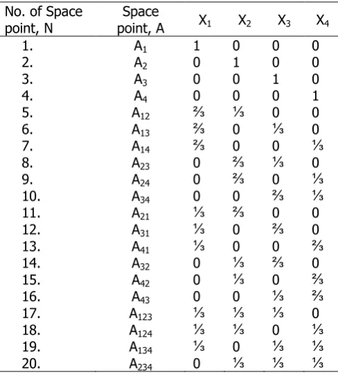
Figure 1: 3D {4, 3} space lattice design

Table 1: Pseudo-components for {4.3} Simplex

Lattice

No. of Space

point, N point, A Space X1 X2 X3 X4

1. A1 1 0 0 0

2. A2 0 1 0 0

3. A3 0 0 1 0

4. A4 0 0 0 1

5. A12 ⅔ ⅓ 0 0

6. A13 ⅔ 0 ⅓ 0

7. A14 ⅔ 0 0 ⅓

8. A23 0 ⅔ ⅓ 0

9. A24 0 ⅔ 0 ⅓

10. A34 0 0 ⅔ ⅓

11. A21 ⅓ ⅔ 0 0

12. A31 ⅓ 0 ⅔ 0

13. A41 ⅓ 0 0 ⅔

14. A32 0 ⅓ ⅔ 0

15. A42 0 ⅓ 0 ⅔

16. A43 0 0 ⅓ ⅔

17. A123 ⅓ ⅓ ⅓ 0

18. A124 ⅓ ⅓ 0 ⅓

19. A134 ⅓ 0 ⅓ ⅓

20. A234 0 ⅓ ⅓ ⅓

1.3 Pseudo - Components in Mixture Design In mixture design, Pseudo – components are referred to as imaginary or coded variables used to simplify design construction and model fitting, thereby reducing the correlation between component bounds in constrained designs. This reduction in the correlations between the coefficients is achieved through the transformation of the “actual components, S” to the pseudo-components, X”. Pseudo-components, in effect, rescale the constrained data area so that the minimum amount allowed (the lower bound) of each component is zero in mixture designs as in Scheffe’s model [3].

2. SCHEFFE’S MODELS IN MIXTURE DESIGN Scheffe’s Models are most times referred to as the mixture models. They differ from the usual regression model due to the correlation between all the components in the mixture designs. Another difference is that the intercept term in the model is not usually included in the regression model [3]. In mixture experiments, the levels of individual components of the mixture are not independent [9]. Assuming the mixture to be a unit quantity, then the sum of all proportions of the component must be unity. That is,

(or ) ( a)

∑ x

(or ) ( b)

Thus, Equation (4) implies that Xi component of the

mixture is within the limits:

( ) The standard form of the full cubic mixture model is given as [9]:

(y) ∑

∑ ∑

∑ ∑ ( )

∑ ∑ ∑

( )

where, = linear blending portion due to the pure blend, = 1 and = 0; ; ( ) Expected response. represents the quadratic nonlinear

blending between component pairs, whose parameters may be either synergistic or antagonistic blending. represents the full cubic nonlinear

blending among component sets of 3, whose parameters may be either synergistic or antagonistic blending.

(4)

2.1 Relationship between the Pseudo and Actual Components

In Scheffe’s mixture design, the Pseudo – components, Xi have relationship with actual

components, Si. The relationship between X and S as

expressed by [9] is given as:

A S A

S or A S

_S

A A

S ( ) where: A _{; A is the actual – pseudo}

proportionality coefficient.

Equation (7) is used to determine actual component of the mixture when the Pseudo components are known, and vice versa.

For q components, and in keeping with the principle of absolute volume, the sum of the actual components mixture in a given factor space is giving as [9]:

S ∑ S

S S S S S ( )

Dividing Equation (8) by the sum of the actual component mixture gives:

( ) Where, S S S S S S S S S

S S Thus, the general form of ith_{factor space is:}

S

S (i , , , q) ( ) Equation (10) is the proportion of the ith_constituent

component of any considered mixture design. As in a general mixture problem, the measured response is assumed to depend only on the proportions of the ingredients in the mixture, and not the amount of the mixture. Therefore, modelling, consequent on experimentation can be based on the actual and pseudo components. Thus, the transformation of the actual components, Si into

actual ratio components, Zi is jettisoned [3].

Then, expressing the actual – pseudo proportionality coefficient expression (Equation (7)) in matrix form is;

[A] [ ] [S] [S]

_{[ ] ( )}

In [3] this expression was developed to mean the inverse or transpose matrix of the actual components corresponding to the pure blend Pseudo – components of space points as follows:

[A] [S] _[S] _{( )}

[A] is defined in (13) below this page.

2.2 Determination of Actual Components of the Nonlinear Blending Mixture, S’

N,q

In [3] the expression given for the other actual components of the binary mixture, S’

N,q for the remaining N – q factor points was:

[ S ,

S ,

] [ s ,

s ,

s , ]

[ , , , , ]

[S , ] [A] [ , ] [S] [ , ] ( )

These derived actual components corresponding to the remaining N – q lattice points of the pseudo – components mixture proportions are used as other mixture proportions in the experimentation so as to obtain their corresponding responses.

3. Formulation of the Modified and Generalized Full Cubic Polynomial Mixture Model and Design Response Coefficients

Scheffe’s full cubic polynomial in Equation (6) possesses some characteristics which do not agree to mixture design expressions in Equations (1) and (3). These characteristics limit the application of the model in mixture design. Among these, the drawbacks identified are as follows:

_____________________________________

[A]

[ a ,

a ,

a , ] [

s ,

s , ] [

s ,

s , ]

(5)

(i) It does not make provision for instances when in the second and third terms of the equation, which would be the case in full cubic polynomial.

(ii) In a third – degree space lattice, the lattice coordinates, pseudo – components, Xi are

defined in Equation (1) as:

, , , , , , ,

Hence, the Scheffe’s model in Equation (6) does not clarify the fact that , are equal for full cubic polynomial at the centroid of the lattice body within I, j, k coordinate.

That is,

(i, and , , , , q i ) ( )

Thus, Equation (6) is modified to take into consideration these drawbacks as follows:

(y) ∑

∑ ∑

∑ ∑ ( )

∑ ∑

( )

∑ ∑ ∑

( ) ( )

Rearranging Equation (16) further gives:

(y) ∑

∑ ∑

∑ ∑ ( )

∑ ∑

∑ ∑ ( )

∑ ∑ ∑

( ) ( )

Expanding the Equation (17) gives:

(y) x

( ), ( ) ( )

( ), ( ) ( ( ) )

,( ) ( ) ( )

,( ) ( ) ( ( ) )

( )( ), ( ) ( ) ( )

In a pure mixture response at ith_{point on the factor}

space, yi, component Xi =1 and components Xj, Xk . .

. Xq are all equal to zero. Then, Equations (17) or

(18) becomes:

(y) y ( ) Thus, in pure mixture point, it can be generalized that:

y (i , , , , q ) ( ) y y ( ) For the binary mixture space point, say, Aij,

lying on the borderline i – j of two components Xi and

Xj, when Xi > Xj, that is, when Xi = ⅔ and Xj = ⅓,

while other components are zeros. The response at this point is yij. Then, Equations (17) or (18)

becomes:

(y) y

( )

y

( ) For the binary mixture space point, say, Aji, lying on

the borderline i – j of two components Xi and Xj,

when Xj > Xi, that is, when Xj = ⅓ and Xi = ⅔, while

other components are zeros. The response at this point is yij. Then, Equations (17) and (18) becomes:

(y) y ( )

( )

y

( ) For the thrice mixture space points, say, Aijk, lying on

the body of components Xi, Xj and Xk, that is, when Xi

= Xj = Xk = ⅓, while other components are zeros at

any space point, the response at this point is yijk.

Then, Equations (17) or (18) becomes:

(y) y

( )

y

( ) Solving Equations (22) and (23) simultaneously for

and :

{ (y

)

(y

) }

{ ( y

)

(y

(6)

y y

(

)

y y

y y y ( y) ( )

Substituting the expression in Equation (25) into

Equation (23) gives as follows:

y

( y y )

y y y ( y) ( )

Substituting Equations (25) and (26) into (24) gives

as follows:

y

y y y y y y

y y y

[y (

y y y

y y y )]

y y y y y

y ( )

Equations (17) and (18) are the generalized mixture design model for the full cubic polynomial of q variables mixture lattice. The term, yi, yij, yji and yijk

correspond to the mixture response at the respective space points i, (ij, ji) and ijk of the actual pure blend, Si for i = 1, 2, 3, …, q (principal points); derived

actual binary blends, Sij and Sji; and derived actual

thrice blend, Sijk respectively, which are obtained

from the laboratory experiments. The coefficients, , , , are defined in Equations (25),

(26) and (27).

4. SCHEFFE’S MODEL AND CONTROLLED EXPERIMENT

The new set of pseudo – components are also systematically selected in the control mixture design proportions; while their actual interacting component mixture, Si corresponding to the control pseudo –

component are determined in the similar manner the inter - component mixture proportions are determined in the main experiments. The pseudo –

components can be of any degree and must conform to Equation (4).

In a controlled experiment, the number of new sets of factor space points should be greater or equal to N space points of the original factor space. This number is required to confirm the adequacy of the model developed in Equations (17) or (18).

Just as in the model experiment, two (or more) parallel and simultaneous experiments are carried out (replication principle) in control experiments. The average response of the replication of each experiment gives a valid and more reliable estimate which is possible with one observation only. This set of mixture proportion can be denoted as: C1, C2, C3,

C4, C5, . CN-1, CN and CN+d.

5. SCHEFFE’S MODEL VALIDATION AND ADEQUACY

The results of the developed model in Equations (17) or (18) is tested for adequacy in relation to the experimental results in the control tests. These experiments which are replicated at least in three places for each design point in the main and control tests are evaluated for adequacy at each level (parallel test) and over the entire experiment (vertical test).

Replicate test run is necessary due to human inconsistency, variation in test tools or equipment and environmental factors such as change in humidity, temperature pressure, etc, which usually affect the experimental results. The mean response of the replication of each experiment gives a valid and more reliable estimate than which is possible with one observation only. The variance of the replicate response at each design point is evaluated. The NULL HYPOTHESIS, Ho and the ALTERNATE

HYPOTHESIS, HA are tested at a specified significance

level, α, which represents the maximum tolerable risk of incorrectly rejecting the null hypothesis, Ho.

Among the tests used to check the significant levels of difference between model and experimental responses include t – test, F – test, Z – statistics and X2_{– statistics.}

[10] gave the expression for the replication variance, at each design point as:

S

∑( )

( ) ( )

where Yi is the individual replicate responses at each

(7)

for the replicate responses at each control point and v; and Y is the mean of the responses for each control point. That is:

∑

( ) ( )

Then, the replication variance across all the points of observation, S will be the sum of the individual replicate variances, S for each design point divided by the degree of freedom of the whole points of observation, Ve. That is,

S ∑ S

∑ S

( ) ( )

Therefore, the random error or standard deviation or replication error value becomes:

√S √( ∑ S

) √(

∑ S

) ( )

5.1 Student t – Test Method

The t test (also called Student’s t – Test) compares two “means” and tells if they are different from each other. The t – test also defines how significant the differences are. In other words, it reveals if those differences could have happened by chance [3]. As cited by [11] and [12] the expression for t – test variance in replicate experimental response is given as follows:

t √

√ ( ) where, n is the number of parallel observations at every point, Sy is the replication error of the entire N

design points in the control experiments, t is the t – statistics and is the estimated standard deviation or error.

The method of obtaining the t – variance using Equation (32) is cumbersome. Hence, [3] gave an advanced and simpler expression for obtaining the t – test variance in replicate experimental response. Their equation gives exactly the same value obtained using Equation (32). The equation is given as follows [3]:

t ∑( )

√_{( )}( ∑( ) (∑( )) )

√( ) ∑( )

√( ∑( ) (∑( )) ) ( ) Ye and Ym are the average experimental and model

responses respectively.

N is total design points in the control experiments, t is the variance from the t – statistics.

The t – value obtained in Equations (32) and (33) are usually the same. They are compared with the one from the standard statistical table according to [13] at enhanced ₍⁄ ) significant level and degree of freedom, Ve. That is, ( )( ). When the t – value

from the standard statistical table, ( )( ) is

greater than those of the t-values obtained in either Equations (32) and (33), the Null hypothesis is accepted and the model is adequate. Otherwise, the Null hypothesis is rejected, the Alternate hypothesis is accepted and the model is not adequate.

5.2 F – Statistics (Fisher) Test Method

This test compares the variance from the model response, Si with that from the experimental

responses. The equation for Fisher test is given as [11]:

explained ariance unexplained ariance

S

S ( ) where,

S or S S ∑( y̅ )

y̅ ∑

y̅ ∑ ( ) Se2 and Sm2 are variances from the experimental and

model responses

S12 is the greater of Se2 and Sm2; S22 is smaller of the Se2

and Sm2

Ye and Ym are experimental and model responses;

and are mean values of experimental and model responses; N is the sample group or total control space points.

(Degree of freedom of design points) ( )

Fisher’s tests the adequacy of the model by comparing the responses of the experimental and model results in the control sample group. The Null Hypothesis is accepted and Alternative Hypothesis rejected if and only if:

( , )

( , ) ( )

where, [13] gave critical values of the ( , )

distribution in which and have their usual meaning; and are the number of degrees of freedom defined in Equation (37).

(8)

in the third-degree mixture design model. Among these limitations are: (a) It does not make provision for instances when Xi < or > Xj in the second and

third terms of the equation, which would be the case in full cubic polynomial, (b) it does not clarify the fact that Xi, Xj and Xk are equal for full cubic polynomial

at the centroid of the lattice body within any i, j, k design space point. These characteristics negate the principle of dependency of the individual components of any design mixture space.

The present work further modified the cubic mixture polynomial, taking into account the deficiency of the Scheffe’s full cubic mixture models. Consequent upon this, a generalized third-degree mixture model was developed for Nth_{components mixture design. Test}

for mixture model adequacy which can be developed from the generalized equation herein are outlined, while the procedure for accepting Null or Alternate hypotheses is discussed and presented.

Based on the new model formulated, the following recommendations are made:

(a) The present third-degree Scheffe’s model developed in this study should be adopted by researchers and practicing engineers for use in larger variable space engineering mixture design model formulation.

(b) The systematic and procedural approach to mixture design for Null and Alternate hypotheses selection criteria outlined in this study is convenient for use in experimental or empirical studies.

(c) The adequacy test methods (Student t – test and Fisher’s F – test) in response surface methodology outlined in this work is very convenient for use in experimental or empirical studies.

7. REFERENCES

[1] K. Ghavami, "Non-conventional Materials and Technologies: Applications and future tendencies," Bath, 2009.

[2] R. H. Myers and D. C. Montgomery., "Response Surface Methodology: Process and product optimization using designed experiment," A Wiley-Interscience Publication, 2002.

[3] O. A. Oguaghamba and B. O. Mama, "Generalized Scheffe's second degree mathematical models approach in engineering mixture design," in 16th Intern. Conf. & AGM of Nigerian Institute of Civil Engineers on Transforming National Economy through Sustainable Civil Engineering Infrastructures – Engineering Solutions to Problematic Soils and Allied Construction Materials, NICE 2018, Calabar, October 24 – 26, pp. 32–44. 2018 [4] D. C. Montgomery, Designs and Analysis of

Experiments, New York: John Wiley and Sons., 6th ed., New York: John Wiley and Sons, 2005. [5] A. Carpi and A. E. Egger, "Experimentation in

scientific research," Vision learning, Vols. POS - 1, no. 7, 2008.

[6] F. O. Okafor and O. A. Oguaghamba, "Procedure for optimization using Scheffe's models," Journal of Engineering Science and Application (JESA), vol. 7, no. 1, pp. 36 - 47, 2009.

[7] R. House, "Simplex-lattice designs," 10 August. [Online]. 2017.

[8] H. Scheffe, "The simplex-centroid design for experiments with mixtures," Journal of Royal Statistical Society, vol. 25, no. B, pp. 235 - 251, 1963.

[9] H. Scheffe, "Experiments with Mixtures," Journal of Royal Statistical Society, vol. 20, no. B, pp. 344 - 360, 1958.

[10] H. Cramer, Mathematical Methods of Statistics, Bombay: Asia Publishing House, 1962.

[11] C. E. Okere, N. N. Osadebe and D. O. Onwuka, "Prediction of flexural strength of soilcrete blocks using Scheffe’s simplex lattice design," International Journal of Computer Science and Engineering, vol. 2, no. 1, pp. 52 - 60, 2014. [12] S. Akhnazorova and V. Katarao, "Design of

Experiments – Part II," in Experiment Optimization in Chemistry and Chemical Engineering, Moscow, Mir Publishers, p. 150– 309, 1982.