Optimal Imperfect Production Inventory Model under Joint Effect of Machine Breakdowns and System Reliability

Vol. 14, No. 2, 2017, 277-291

ISSN: 2279-087X (P), 2279-0888(online) Published on 13 September 2017

www.researchmathsci.org

DOI: http://dx.doi.org/10.22457/apam.v14n2a11

277

Annals of

Optimal Imperfect Production Inventory Model under

Joint Effect of Machine Breakdowns and

System Reliability

Prasanta Kumar Ghosh

Department of Mathematics, Y.S.Palpara Mahavidyalaya, Palpara Purba Midnapore, W.B., India. E-mail:[email protected]

Received 30 August 2017; accepted 10 September 2017

Abstract: This paper investigates the role of reliability parameter of the imperfect production system with random machine breakdown and stochastic repair time. Here I assume that shifting time of the production system from ‘in-control state’ to ‘out-control state’ and the time of machine breakdown are both random. Moreover, the machine repair time is stochastic and independent of the machine break-down rate. To make the research a more realistic one, a relation between reliability parameter and machine breakdown parameter has been established so, that smaller value of reliability parameter indicates long run of production process, lesser imperfect items and negligible number of machine breakdown. Finally, the model is formulated as a profit maximization problem by considering the reliability parameter and production up time as a decision variables. A numerical example is presented to illustrate the impact of profit with different variables in the model. Also, sensitivity analyses are conducted to show how the model reacts to changes in parameters.

Keywords: Imperfect production, machine breakdown, stochastic repair time, reliability of the production system.

AMS Mathematics Subject Classification (2010): 90B05 1. Introduction

278

The authors in[7], analyzed a production-inventory model using queuing theory techniques. An unreliable M/G/1 queuing system was considered, and a maintenance process was also introduced in addition to the failure process of the production facilities. For this case, the Laplace transform of the slack capacity was derived. In [4], Groenevelt et al. proposed two production control policies to address the EMQ model with machine failures and they focused on the effects of machine breakdowns and corrective maintenance on the economic lot sizing decisions. The first policy considers that the production of an interrupted lot will not be resumed after a breakdown (i.e., the no resumption or NR policy), while the second assumes that the production of an interrupted lot resumed immediately after production is restored and if the current on-hand inventory is below a certain threshold level (i.e., the abort-resume or AR policy). In the article[8],it was follows that a broad class of production-inventory systems in which a number of producing machines are susceptible to failure following which they must be repaired to make them operative again. The machines’ production can also be stopped deliberately due to stocking capacity limitations or any other relevant considerations. In[4], authors has derived some structural properties of the modified lot sizing model with exponential failure. However, they do not give a procedure to determine the optimal lot size. In [6], Chung derived the bounds for the optimal lot size and he obtained some results with these bounds. Kuhn [5] addresses the dynamic lot sizing model with the assumption that the equipment is subject to stochastic breakdowns and considered two different situations. Firstly, after a machine breakdown the setup is totally lost and new setup cost is incurred. Secondly, the cost of resuming the production run after a failure might be substantially lower than the production setup cost. In [11], it was assumed that the number of failures in a production run is Poisson distributed while the repair times are random and can assume any general distribution. Upon failure, the machine will receive immediate service, and the demand will be met from inventory. In the article [20], presented a model of single-machine scheduling problem. The machine is failure-prone and subject to random breakdowns. The processing time is a deterministic sequence that is randomly compressible, which may be from the introduction of new technology or addition of new equipment. In [21,22 ,23], studied the optimal production run time in an EMQ model with imperfect rework and Poisson machine breakdowns under the abort/resume (A/R) control policy. In their proposed system, a random defective rate is assumed and all defective items are reworked at the end of regular production, and there exists a certain percentage of rework failures. The system is subject to random breakdowns and the A/R inventory control policy is adopted when breakdowns occur. Mathematical modeling was used, and theorems related to conditional convexity and bounds of optimal production run times were proposed and proved in their study. A recursive searching algorithm was developed to locate the optimal run time that minimizes the expected production “inventory costs. Some other models concerned with inventory control and machine failure have also been investigated, cf. [1,2,12,15,16,17]. Further effect of stochastic machine breakdown was investigated in [3,13,14]. Again different type of inventory model with different type of demand is studied in [9,18,19].

Breakdowns and System Reliability

279

established so that smaller value of reliability parameter indicates long run of production process, lesser imperfect items and negligible number of machine breakdown. Finally, the model is formulated as a profit maximization problem by considering the reliability parameter and production up time as a decision variables.

2. Assumptions and notations

The following assumptions and notations are adopted for this model.

2.1. Assumptions

(i) The production rate is constant and deterministic.

(ii) From the beginning of the production process, the machinery system is in the ’in-control’ state and goes to ’out of control state’ when life time of the system is T =t, where T follows a probability densityfunction

( ) = t, > 0, 0 < <

f t θe−θ θ t ∞ and produces imperfect quality items .

(iii) Full inspection of the production process is consider. Only the β( <o β< 1) times of total imperfect quality items are sale at a low price rate(reduction sale). and (1−β) times of imperfect quality items are rejected with a certain environmental consciousness cost.

(iv) (constant) be the demand rate of perfect quality items throughout the production cycle.

(v) In big-bazaar market or occasional market , with proper advertisement about the product , the demand is exponentially increases with low price rate.So, we

consider the demand rate, = 1 2

s_max s_i s_i s_min

e δ δ δ

− −

+ is for acceptable imperfect quality items. where δ1andδ2both are positive constant.

(vi) Immediately after the end of production up time, reduction sale of acceptable imperfect items are consider.

(vii) Shortages are not allowed but due to greater machine maintenance time than production down time of perfect item,lost sale will occur.

(viii) In case of machine breakdown ,repair time is stochastic and independent of machine break down.

(ix) For development of the reliability of the production system along with product, we consider production cost related to reliability parameter as

( , ) = d

p m

c

c t c p

p

θ ν

θ

+ + .Where c and m c are the material cost and d

development cost per item per unit time and ν is constant. (x) The time horizon is infinite.

λ

280 2.2. Notations

p The production rate is constant and deterministic. λ Demand rate of perfect quality items.

δ Demand rate of acceptable imperfect quality items. θ Reliability parameter.

p

I Inventory of the perfect quality items at time t.

d

I Inventory of the imperfect quality items at time t. Q Total Inventory in the production cycle.

1

t Time of production stop.

p

t Time when machine breakdown occur.

2

t Time of perfect quality items are exhaust.

3

t Time of imperfect quality items are exhaust. K Setup cost per cycle of production system.

h

c Holding cost per item per unit time.

p

c Production cost per unit item per unit as a function of reliability parameter.

dd

c Disposal cost per unit item/time.

p

s Price rate of perfect quality items.

i

s Price rate(reduced) of acceptable imperfect quality items. ( )

E Q Expected inventory holding in the production cycle.

( )

E HC Expected inventory holding cost. ( )

E P Expected production quantity in the production cycle.

( )

E PC Expected production cost. ( )

E T Expected duration of the production cycle.

( )

E CLS Expected lost sale cost.

( )

E DC Expected disposal cost. ( )

E TC Expected total cost. ( )

E SR Expected sales revenue.

1

( , )

EP t θ Expected profit per unit time.

3. Mathematical formulation of proposed inventory model and discussion

Considering an imperfect production process in which it has two states ’in-control-state’ and ’ out-of-control-state’.The production process shifted to ’out-of-control’ state from ’in -control’ state and as a result production of imperfect items aries. Due to long run production process with machine, the system goes to ’out-of-control’ state and consider it is as failure , as a result produces more imperfect items than the ’in-control’ state.

Breakdowns and System Reliability

281 Number of failure

=

Total number of working hours

θ , that is θ is failure per unit time. For example

= 0.02

θ , means ,the system goes to ’out of-control’ state one time for a 50 hours working period of production run.Basically θ indicate the hazard rate of the production system , which is combination of random failure and wear-out failure from ’in-control’ state to ’out-of-control’ state.The failure of machinery systems are either due to random failure or wear-out failure, so, reliability of the system can be expressed as

1 2

( ) = ( ) ( )

R t R t R t , where R t₁( ) and R t₂( ) are the reliability due to random failure ,independent of time and reliability due to wear-out . Since the hazard rate due to random failure is independent of time,so, reliability of the system due to random failure with constant hazard rate is 1( ) =

t

R t e−θ . Again by appropriate maintenance policies we can reduce the failure due to wear-out. As a result our study must be concentrate on the failure due to random chance.And therefore corresponding reliability function of the machinery system is defined at time ’t’ as R(t) = e−θt, where > 0, t > 0θ .

0

( ) 1- ( ) 1- t ( )

R t = F t =

∫

f t dt.So, f t( ) dF t( ) e- t , 0 and t 0 dt

θ

θ θ

= = > > .

Here ( )f t and F t are the density and distribution function of the life time ( i.e, stay in ( ) the ’in-control’ state )of the production process .The production process is more reliable if is small and due to that the production process may stay long period in the ’in-control’ state. As, a result lesser quantity of imperfect items is produced, which implies

is the product reliability of the production process it means less imperfect items more reliability of the product. But during long run production process, the percentage of imperfect items increases, in the same time production process shifted to ’out-of-control’ state and causes machinery system of the production process is breakdown.

Since the production of imperfect items and breakdown of the machinery system related to the reliable parameter , so, the probability of the imperfect quality of items of total production follow the probability density function f t( ) =θe−θt. If p be the production rate ,then the expected rate of imperfect product at time t is p(1−e−θt) and consequently the rate of perfect quality item is pe−θt. In the same time machine breakdown of machinery production system follow the probability density function

( ) =t e αt

φ α − _{,α = (1−c)θ or (1+c)θ, (0 <c< 1). When α = (1−c)θ , the mean time}

of machine breakdown is greater than the mean time of machinery system shifting from ’in-control’ state to ’out-of-control’ state i.e. probably the machine breakdown occur in the ’out-of-control’state.And α = (1+c)θ , indicate the mean time of machine breakdown is lesser than the mean time of machinery system shifting from ’in-control’ state to ’out-of-control’ state i.e. probably the machine is breakdown in the ’in-control’state. Smaller value of θ indicates long run of production process in the ’in-control’ state, lesser imperfect items and negligible number of machine breakdown. The perfect and imperfect quality items are separates by a inspection section. This section select the acceptable quality of imperfect items, β times of the total imperfect quality items which are suitable

θ

θ

282

for sale at a low price rate( i.e the reduction sale) and (1−β) times of imperfect quality items are rejected (scrapped) with environmental consciousness with a certain cost. For the production cycle, Ip( )t and Id( )t denotes the inventory level at time t of perfect

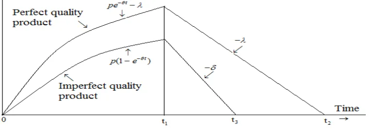
quality items and imperfect quality items respectively. The inventory levels of perfect quality items increases at a rate pe−θt−λ and inventory levels of imperfect quality items increase at a rate p(1−e−θt) up to time t=t1, where is the production up time. The

demand of perfect quality items are meet with a rate λ throughout the production cycle. Immediately after the production run, the acceptable quantity of imperfect items are sale

at rate = 1 2 ( )/( )

s_max s_i s_i s_min

e

δ δ δ+ − − up to time t=t₃, when the imperfect items are exhaust. The behavior of such a unified system is depicted in Figure 1.

Figure 1: Inventory level of the production system with respect to time.

4. The inventory level are governed by the following differential equations 4.1. Perfect quality inventory

The governing differential equation of the perfect quality iitem is

1

1 2

( ) ; 0

=

;

t p

dI t pe t t

dt t t t

θ _λ λ

−

 _{− ≤ ≤}

 

− ≤ ≤

 (1) with I_p(0)=0and I_p( )t₂ =0 .

4.2. Imperfect quality inventory

The governing differential equation of the imperfect quality item is

1

1 3

(1 ) ; 0 ( )

=

;

t

d p e t t

dI t

dt t t t

θ β

δ −

 _{− ≤ ≤}

 

− ≤ ≤

 (2) withI_d(0)=0 and I_d( )t₃ =0.

where β , (0< <β 1) is the portion of imperfect items ,which are produced during the production run.

From (1) and (2), it follows

Breakdowns and System Reliability

283

1

1

1 2

(1 ) ; 0

( )

(1 ) ;

t

p

t

p

e t t t

I t p

e t t t t

θ θ λ θ λ θ − −  − − ≤ ≤  =  _{− − ≤ ≤}  (3) 1 1

1 1 1 3

( 1) ; 0

( ) =

( 1) ( ) ;

t

d

t

p

e t t t

I t

p

e t t t t t t

θ θ β _θ θ β _{θ δ} θ − −  + − ≤ ≤    _{+ − − − ≤ ≤}  (4)

from the boundary condition , 1

2 (1 )

t

p

t e θ

θλ −

= − and 1

3 1 ( 1 1)

t

p

t t β e θ θt θδ −

= + + −

For feasibility,t₂>t₁ and t₃>t₁ implies 1

1

(1 t)

p −e−θ >θt and 1

1

( t 1) 0

p

e θ t

β _θ

θ − + − > . Inventory for the perfect quality items is

1 2 ₁

0 ₁

= t[ (1 t) ] t [ (1 t ) ]

p

t

p p

Q e θ λt dt e θ λt dt

θ θ

− −

− − + − −

∫

∫

2 2 2

2 1

1 1 1

2 2 2 2 2

= ( )

2 2

t pt t t

p p p p p

e θ e θ e θ

θ

λθ θ θ λθ λθ

− − −

− + − + + ( 5)

Inventory for the imperfect quality items is

1 3 ₁

1 1

0 ₁

= t[ ( t 1)] t[ ( t 1) ( )]

d _t

p p

Q β eθ θt dt β eθ θt δ t t dt

θ θ

−

− _{+ − + + − − −}

∫

∫

2 2 2 2 2 2 2 2

2 1

1 1

2 2 2 2

= ( ) ( ) ( ) ( )

2 2

2

t

p p p p p p p p

t t e θ

β β β β β β β β

δ θ θδ

θ θ δ θ θ δ

−

+ + + − + − +

2 2 2 2

2 1 1 1 2 2 t t p p

t e θ e θ

β β

θδ θ δ

− −

+ + (6)

Hence the total inventory is

1 1 2 1

2

1 2 1 3 1 4 5 1 6

= _{d p} t t t

Q Q +Q = +c c t +c t +c e−θ +c t e−θ +c e−θ (7) where

2 2

1 2 2

1 (1 )

= ( )

2

p p

c β β

λ δ

θ θ

−

+ − ,c₂ = pβ(1 βp)

θ δ

− + , ₃ = (1 )

2

p p

c β β

δ +

2 2

4 2 2

(1 ) 1

= p p ( )

c β β

λ δ

θ θ

− _{− +}

,

2

5 = (1 )

p p c β θ + δ , 2 2 6 2 1 = ( ) 2 p c β λ δ θ +

4.3.Case 1: Machine breakdown occur and stochastic machine maintenance time exceed production down time

For greater value of reliability parameter , the machinery system of production process breakdown and suppose it is occur at the time point =t t and follow the probability p

density function ( ) =f tp e tp, > 0

α

284

2 2

1 2 3 4 5 6 1

2

2 _{1 1 1}

1 2 1 3 1 4 5 1 6 1

; =

;

t_p t_p t_p

p p p p

t t t

p

c c t c t c e c t e c e t t

Q

c c t c t c e c t e c e t t

θ θ θ θ θ θ − − − − − −  _{+ + + + + ≤}   + + + + + ≥

 (8)

2

1 2

1 2 3 4 5 6

0

( ) = t( p p tp p tp tp) ( )p p

E Q

∫

c +c t +c t +c e−θ +c t e−θ +c e−θ f t dt

2

2 1 1 1

1 2 1 3 1 4 5 1 6

1

( t t t ) ( )p p

t c c t c t c e c t e c e f t dt

θ θ θ

∞ _{− − −}

+

_∫

+ + + + + (9)

which gives

3 5 6 3 3

2 4 1 2 1

1 2 2 1 2

( ) ( ) (2 )

5 5 6

4 1 1 1

1 2

2 2 2

( ) = ( ) 2 ( ) 2 ( ) 2 ( ) t t

t t t

c c c c c

c c c

E Q c t e e

c c c

c

e t e e

α α θ α α θ θ α α α α α θ α θ α θ α α α α α θ θ α θ θ α α θ α θ − − − + − + − + + + + + + − − + + + + + − + + + + + + (10)

Hence expected inventory holding cost is

3 5 6 3

2 4 2 1

1 2 2 2

2 2 ( ) = [ ( ) 2 ( ) t h

c c c c

c c c

E HC c c α α e α

α α θ α θ α θ α α α

−

+ + + + + − +

+ + +

( ) ( ) (2 )

3 1 4 5 1 5 1 6 1

1 2 1

2 2

( ) ]

2

( )

t t t t

c c c c c

t e α θ α e θ α t e α θ θ e θ α

α α θ θ α α θ α θ

− − + − + − +

− + − + +

+ + + + (11)

Expected production in production run is

1 ₁

1

0 ₁

( ) = t( _p) tp _p ( ) tp _p = (1 t )

t

p

E P pt αe α dt pt αe α dt e α

α ∞

− − −

+ −

∫

∫

(12)

Expected production cost is

1 1

( ) = (1 t ) = ( d ) (1 t )

p m

c

p p

E PC c e c p e

p

α _ν α

α θ α

− −

− + + − (13)

4.4. Machine maintenance time is stochastic

When the machine breakdown occur with in the production run time,the corrective maintenance of the machine is required and let machine maintenance time is stochastic which is uniformly distributed in(0, )µ with density function

1 ; 0 ( ) = 0 ; t g t elsewhere µ µ  _{≤ ≤}    

Therefore Expected duration of the production cycle is

1 1

2 2 2

0 ₁ 0 ₂

( ) = t tp _p tp _p t (( ) ( )) tp _p

t t

E T

∫

t αe−α dt +

∫

∞tαe−α dt +

∫ ∫

∞ t−t g t αe−α dt dt

1

2 2

0 ₂

= ( ) t ( ) ( ) tp _p

t

E t +

∫ ∫

∞ t−t g t αe−α dt dt (14) Here t₂ represent the end of the production cycle and 3rd term in the above expression

represent the extra time for machine maintenance exceed .

1 2

0

( ) = t (1 tp) tp p

p

E t e θ αe α dt

λθ

− −

−

∫

1

1

(1 t ) tp _p

t

p

e θ αe α dt λθ

∞ − −

+

_∫

− ( )₁

= (1 )

( )

t

p

e θ α λ α θ

− + − + Again expected extra time for machine repair is

2

Breakdowns and System Reliability

285

1

2 0 =₂

( ) = t ( ) ( ) tp _p

t t

E ET

∫ ∫

∞ t−t g t αe−α dt dt

2

(2 ) ( )

2 1 1 1

2 2

1 2 ( )

= [( ) (1 ) (1 ) (1 )]

2 2

t p t p p t

p e α α e θ α α λµθ e θ α

λµθ θ α θ α µλ θ − − + − − + − − + − + − + +

Above two relation together gives,

2

( )

2 1 1

2 2

2

(2 )₁

1 2

( ) = [( ) (1 ) (2 ) (1 )

2 (1 )] 2 t t t p

E T p e p e

p e α θ α θ α α λµθ µλθ θ α µλ θ α θ α − − + − + − − + − − + + − + (15)

Expected lost sale cost for perfect quality item is

2

( )

2 _{1 1}

2

2

(2 )₁

2

( ) = [( ) (1 ) (2 )(1 )

2 (1 )] 2 t t p t s _p

E CLS p e p e

p e α θ α θ α α λµθ µλθ θ α µλθ α θ α − − + − + − − + − − + + − + (16)

Expected disposal amount of imperfect product in the production process is

( )

1 1

(1 ) (1 )

( ) = (1 ) [ ]

t t

e e

E DIS p

α θ α β α α θ − − + − − − −

+ (17) Expected disposal cost for environmental point of view is

( )

1 1

(1 ) (1 )

( ) = (1 ) [ ]

t t

dd

e e

E DC c p

α θ α β α α θ − − + − − − −

+ (18) Expected total cost Setup cost(including inspection cos Expected Production cost Expected inventory holding cost Expected lost sale cost Expected disposal cost .

( ) 1 1 3 2 4 1 1 2 2

(1 ) (1 )

( ) = ( ) (1 ) (1 ) [ ] [

t t

t d

m dd h

c p e e c c c

E TC K c p e c p c c

p α θ α α α ν β θ α α α θ α α θ α − − + − − − + + + − + − − + + + + + + ( ) ( )

5 6 2 3 1 3 1 4 5 1 5 1 6

1 1

2 2 2

2 2 2

( ) ( )

2 2

( ) ( )

t t t t

c c c c c c c c c

eα t eα e θ α t e α θ

α θ α θ θ α α α α θ α θ α θ θ α α θ α − − − + − + + + − + − + − + + + + + + + + 2

(2 )1 2 1 ( )1

2

2

] [( ) (1 ) (2 )(1 )

2

t sp t p t

e θ α λµθ p eα pµλθ α e θ α

θ α µλθ − + − − + + − − + − − + (19)

4.5. Sales revenue

We consider be the price rate of acceptable imperfect quality items, and s be the p

selling price of perfect item, then sales revenue in the complete cycle is

1

1 2 3 1 1

0 _{1 1}

( 1)

= [ ] = (1 )

t

t t t _{p t}

p i i

t t

ps e t

s dt dt s dt e s p

θ θ θ λ λ δ β θ θ − − + − + + − +

∫

∫

∫

(20)

If the machine breakdown occurs at t=t , then expected sales revenue from the p

=E TC =( ) ( )K +

( (E PC))+ ( (E HC))+

( (E CLS))+ ( (E DC))

2

(2 )₁

(1 )]

2

t

p

e θ α

286 complete production cycle is

1 ₁

0 ₁

( 1)

( ) = ( (1 ) ) ( (1 )

t_p

t p tp p tp p t

i p

t

ps e t ps

E SR e s p e dt e

θ θ θ α θ β α θ θ θ − ∞ − + − − − − + + −

∫

∫

( )

1 _{( )} 1 1

1 1

( 1) (1 ) (1 )

) = [1 ] [ ]

t t t

tp p t

i p i

ps

e t e e

s p e dt e s p

θ α θ α α α θ θ β α β θ α θ α α θ − − − + − − + + − − − + − + − + +

Expected profit per unit time (Expected sales revenue Expected total cost) Expected production cycle

( )

1 1

( )₁

1

(1 ) (1 )

( , ) = [1 ] [ ] [ ( )

t t

t

p d

i m

ps e e c p

EP t e s p k c p

p α θ α α θ θ β ν α θ α α θ θ α − − + − + − − − + − − + + + + + ( ) 1 1 3 5 2 4 1

1 2 2

2

(1 ) (1 )

(1 ) (1 ) [ ] [

( ) t t t dd h c c c c e e

e c p c c

α θ α α _β α α α α θ α α θ α θ α − − + − − − − + − − + + + + + + + + ( ) ( )

6 2 3 1 3 1 4 5 1 5 1

1 1

2 2

2 2

( ) ( )

2 ( )

t t t t

c c c c c c c

e α t e α θ α e θ α t e α θ

θ α α α α α θ θ α α θ

− − − + − +

+ − + − + − +

+ + + +

2

(2 ) 2 ( )

6 1 1 1

2

2 2

] [( ) (1 ) (2 )(1 )

2 2

t sp t t

c p

e θ α p e α p e θ α

θ _{λµθ µλθ} α α θ µλθ θ α − + − − + + + − − + − − + + 2 2

(2 )₁ 2 ₁ ( )₁

2 2

1 2

(1 )]]/ [( ) (1 ) (2 )(1 )

2 2

t t t

p p

e θ α p e α p e θ α

α _{λµθ µλθ} α θ α µλ θ θ α − + − − + + − − − + − − + + 2

(2 )₁

(1 )]

2

t

p

e θ α α

θ α

− + −

+ (21) µ must be greater than t₂, otherwise lost sale does not occur, which gives

1 1< (1 ) <

t

t p e θ

λ − − θλµ(22)

5. Solution

Our objective function (expected profit per unit time) EP t( , )₁θ is a function of two variable t₁ and θ, when the design parameter of reliability θ is consider as variable. So, our objective is to find the optimal value of t₁ and θ for which the objective function

1

( , )

EP t θ is maximum. So that the necessary condition for objective function to be

maximised is 1 1 ( , ) = 0 EP t t θ ∂

∂ and

1

( , ) = 0

EP t θ θ ∂

∂ and the sufficient condition

2 1 2 1 ( , ) < 0 EP t t θ ∂ ∂ and 2 1 2 ( , ) < 0

EP t θ θ ∂

∂ and

2 2 2

2

1 1 1

2 2

1 1

( , ) ( , ) ( , ) ( ) > 0

EP t EP t EP t

t t θ θ θ θ θ ∂ ∂ ₋ ∂ ∂ ∂

∂ ∂ for t1> 0 and θ> 0

along with the condition (22) . Now due to highly nonlinearity of EP t( , )₁ θ , the first and second derivatives of this with respect to t₁ and θ are very much complicated. Hence it is difficult to determine closed form solution of t₁ and θ for which the objective

1

( , )

EP t θ is optimum by analytical method. Using MATHEMATICA, we see that, Expected profit per unit time is concave for t₁> 0 and θ > 0.

1

Breakdowns and System Reliability

287 6. Numerical examples

Case-1: (α = (1−c)θ,0 <c< 1).

The parametric values in the model are as k=10000, p=800, 600, 600, 10,

400, 350, 200, 250, 0.75, 2, 25, 10, 10, 50,

0.01, . We analyses the effect of expected profit per unit time on optimum production runtime of the production process and on optimum reliability parameter .

Figure 2: Expected Profit per unit time is concave with respect to both the variable t1

and θ

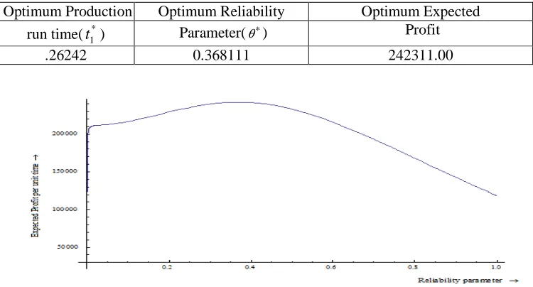
Table 1: Expected optimum profit per unit time, optimum production time and Optimum value of θ.

Optimum Production Optimum Reliability Optimum Expected

run time( ) Parameter( ) Profit

.26242 0.368111 242311.00

Figure 3: Expected Profit per unit time is decreases with respect to increase of reliability parameter

=

λ δ1= δ2= sp=

=

max

s smin= si= β= µ= c_h = c_dd = c_m = c_d =

=

ν c=0.25

θ

* 1

288

Table 2: Expected profit per unit time and Production time for changes of reliability parameter.

Reliability Parameter 0.3 0.35 0.36811 0.37 0.4 Production time 4.66876 5.10589 5.26242 5.27853 5.52572 Expected Profit 240599.00 242176.00 242311.00 242310.00 241855.00

Table 3: Expected production cost per item per unit time for changes of reliability parameter.

Reliability Parameter 0.3 0.35 0.36811 0.37 0.4 Expected production cost 42096.2 40899.0 40335.3 40272.7 39189.7

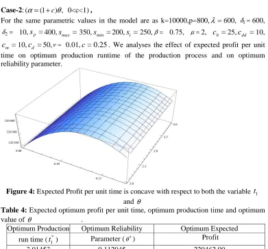
Case-2: (α = +(1 c) , 0<c<1)θ ,

For the same parametric values in the model are as k=10000,p=800, 600, 600,

10, 400, 350, 200, 250, 0.75, 2, 25, 10,

10, 50, 0.01, . We analyses the effect of expected profit per unit time on optimum production runtime of the production process and on optimum reliability parameter.

Figure 4: Expected Profit per unit time is concave with respect to both the variable and θ

Table 4: Expected optimum profit per unit time, optimum production time and optimum

value of θ .

Optimum Production Optimum Reliability Optimum Expected

run time ( ) Parameter ( ) Profit

3.01453 0.112945 220462.00

=

λ δ1=

2

δ = sp = smax = smin = si = β= µ= ch = cdd =

= m

c c_d = ν= c=0.25

1

t

* 1

Breakdowns and System Reliability

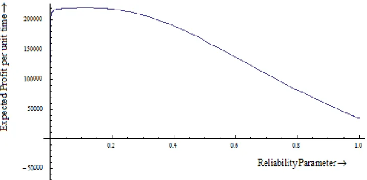
289

Figure 5: Expected Profit per unit time is decreases with respect to increase of reliability parameter

Table 5: Expected profit per unit time and Production time for changes of reliability parameter.

Reliability Parameter 0.08 0.09 0.112945 0.15 0.2 Production time 2.83391 2.88981 3.01453 3.21872 3.52053 Expected Profit 220293.0 220380.0 220462.0 220236.0 219096.0

Table 6: Expected production cost per item per unit time for changes of reliability parameter.

Reliability Parameter 0.08 0.09 0.112945 0.15 0.2 Expected production cost 37077.9 36896.7 36440.8 35604.5 32969.9

7. Conclusion

290 REFERENCES

1. A.J.P.Gharbi, A.C.Kenn and M.Beit, Optimal safety stocks and preventive maintenance periods in unreliable manufacturing systems, International Journal of Production Economics,107 (2) (2007) 422-434.

2. B.C.Giri and W.Y.Yun, Optimal lot sizing for an unreliable production system under partial backlogging and at most two failures in a production cycle, International Journal of Production Economics, 95(2) (2005) 229-243.

3. G.A.Widyadana and H.M.Wee, Optimal deteriorating items production inventory models with random machine breakdown and stochastic repair time, Applied Mathematical Modelling, 35 (2011) 3495-3508.

4. H.Groenevelt , L. Pintelon and A Seidmann.: Production lot sizing with machine breakdowns, Management Science, 38(1) (1992) 104-123.

5. H.Kuhn, A dynamic lot sizing model with exponential machine breakdowns, European Journal of Operational Research, 100 (1997) 514-536.

6. K.J.Chung, Bounds for production lot sizing with machine breakdowns, Computers Ind. Engng, 32 (1997) 139-144.

7. L.Hsu and C.S.Tapiero, Maintenance of an unreliable M/G/l queueing job shop, Queue. Syst., 2 (1987) 333-350.

8. M.Berg, M.J.M.Posner and H.Zhao, Production-inventory systems with unreliable machine, Operations Research, 42(1) (1994) 111-118.

9. M.Mandal and S.K.De, An EOQ model with parabolic demand rate and time varying selling price, Annals of Pure and Applied Mathematics, 1(1) (2012) 32-43.

10. M Shafarali, On a continuous review production-inventory problem, Opns. Res. Lettrs, 3 (1984) 199-204.

11. N.E.Abbound, A simple approximation of the EMQ model with Poisson machine failures, Production Planning and Control, 8(4) (1997) 385-397.

12. N.Rezg, A.Chelbi and X.Xie, Modeling and optimizing a joint inventory control and preventive maintenance strategy for a randomly failing production unit: analytical and simulation approaches, International Journal of Computer Integrated Manufacturing, 18 (2-3) (2005) 225-235.

13. P.K.Ghosh and J.K.Dey, Optimal imperfect production inventory model with machine breakdown and stochastic repair time, World Journal of Research and

Review, 3(1) (2016) 59-65.

14. P.K.Ghosh and J.K.Dey, An imperfect production inventory model with remanufacturing of return and defective items, International Journal of Computer Applications, 150 (8) (2016).

15. R.I.Zequeira, B.Prida and J.E.Valda, Optimal buffer inventory and preventive maintenance for an imperfect production process, International Journal of Production Research, 42 (5) (2004) 959-974.

Breakdowns and System Reliability

291

17. T.Dohi, H.Okamura and S.Osaki, Optimal control of preventive maintenance schedule and safety stocks in an unreliable manufacturing environment, International Journal of Production Economics, 74 (2001) 147-155.

18. W.Ritha and S.R.Jeyakumari, Fuzzy inventory model for imperfect quality items with shortages, Annals of Pure and Applied Mathematics, 4(2) (2013) 127-137. 19. W.Ritha and I.A.Vinoline, Optimization of EPQ inventory models of two level trade

credit with payment policies under cash discount, Annals of Pure and Applied Mathematics, 8(1) (2014) 39-55.

20. X.D.Qi, G.Yin and J.R.Birgd,Single-machine scheduling with random machine breakdowns and randomly compressible processing time, Stochastic Analysis and Applications, 18(4) (2000) 635-653.

21. Y.S.P.Chiu and H.H.Chang,Optimal run time for EPQ model with scrap, rework and stochastic breakdowns,a note, Economic Modelling, 37 (2014) 143-148.

22. Y.S.P.Chiu, K.K.Chen, F.T.Cheng and M.F.Wu, Optimization of the finite production rate model with scrap,rework and stochastic machine breakdown, Computers and Mathematics with Applications, 59 (2010) 919-932.