The Thirty-Third AAAI Conference on Artificial Intelligence (AAAI-19)
Adversarial Actor-Critic Method for Task and
Motion Planning Problems Using Planning Experience
Beomjoon Kim, Leslie Pack Kaelbling, Tom´as Lozano-P´erez
Computer Science and Artificial Intelligence LaboratoryMassachusetts Institute of Technology {beomjoon,lpk,tlp}@mit.edu
Abstract
We propose an actor-critic algorithm that uses past plan-ning experience to improve the efficiency of solving robot task-and-motion planning (TAMP) problems. TAMP plan-ners search for goal-achieving sequences of high-level op-erator instances specified by both discrete and continuous parameters. Our algorithm learns a policy for selecting the continuous parameters during search, using a small training set generated from the search trees of previously solved in-stances. We also introduce a novel fixed-length vector rep-resentation for world states with varying numbers of objects with different shapes, based on a set of key robot configura-tions. We demonstrate experimentally that our method learns more efficiently from less data than standard reinforcement-learning approaches and that using a learned policy to guide a planner results in the improvement of planning efficiency.
Introduction
A task and motion planning (TAMP) problem involves plan-ning a sequence of low-level robot motions that achieves a high level objective, such as cooking a meal, by inte-grating low-level geometric reasoning with high-level sym-bolic reasoning. This typically requires a search in a high-dimensional hybrid space, for a sequence of high-level oper-ators, each of which has both continuous and discrete param-eters. Existing planners (Garrett, Kaelbling, and Lozano-P´erez 2017; Cambon, Alami, and Gravot 2009; Srivastava et al. 2014; Kaelbling and Lozano-Perez 2011) successfully tackle these problems, but they can be very computationally costly, because each node expansion typically requires a call to a motion planner to determine feasibility.
This paper proposes a learning algorithm that learns to guide the planner’s search based on past search experi-ence. We focus on an important subclass of TAMP called geometric-TAMP (G-TAMP), whose emphasis is on geo-metric reasoning rather than symbolic task reasoning. In G-TAMP, the primary interest is achieving a high-level objec-tive by changing the poses of objects using collision-free motions, as shown in Figures 1a and 1b. Whether cooking, cleaning, or packing, all TAMP problems require geomet-ric reasoning. Therefore, any efficiency improvements to TAMP problems, will benefit TAMP more broadly. For
G-Copyright c2019, Association for the Advancement of Artificial Intelligence (www.aaai.org). All rights reserved.
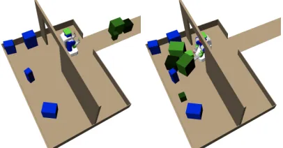
(a) Conveyor belt domain: green objects must be packed in room.
(b) Fetch domain: objects must be removed from path to target object.
Figure 1: Examples of initial (left) and goal states (right).
a policy will constrain the planner’s continuous search space to smaller yet promising regions, making the search more ef-ficient. And, because we will use the policy to guide search, occasional poor action choices will not impact the correct-ness of the actions ultimately selected by the robot.
To learn a policy, we use a dataset of past planning ex-perience. Our premise is that the planner generates operator sequences that yield high rewards. This is based on two ob-servations. First, the planner only adds feasible operator in-stances to its search tree, which allow us to learn to exclude operator instances such as infeasible object placements. Sec-ond, a search tree usually contains states and actions that move closer to the goal based on a heuristic function. Even when the heuristic function is not optimal, this is far more effective than an unguided exploration strategy.
Therefore, we would like to learn a policy that imitates the planner’s operator sequences from the search trees. How-ever, this poses a challenge: from an episode of planning experience, we get a search tree, that contains one solution sequence and manyoff-targetsequences that are feasible but did not get to a goal state (although they might have, had the planner continued expanding them). Since we have both off-target and solution sequences, we cannot simply train a pol-icy that imitates the operator instances on these sequences.
Alternatively, we could completely rely on a reward signal and discard this planning experience dataset, but doing so would be extremely wasteful. Feasible state and operator se-quences are a clearer learning signal than rewards from ran-dom exploration in a high-dimensional state-action space.
Therefore, we propose an actor-critic method that learns a policy by simultaneously maximizing the sum of re-wards and imitating the planning experience. Our algo-rithm, Adversarial Monte-Carlo (ADMON), penalizes oper-ator instances if they are too different from the planner’s se-quences, while learning the Q-function of the sequences us-ing past search trees. ADMONcan be seen as a regularized policy learning procedure, where the regularization encour-ages imitating the planning data.
The learned policy operates on a representation of the planning state. G-TAMP problems usually involve vary-ing number of objects with different shapes, and the ever-changing shape of the robot as it picks, places, and otherwise manipulates the objects in the environment. Thus, encoding the state as a fixed-size vector is not straightforward.
We propose akey configuration representation, inspired by the roadmap approach used in multi-query path planning. This representation copes with different number of objects and different robot and object shapes. Specifically, key con-figurations are a set of robot concon-figurations that were used in past solutions. Given a new problem instance, the collision state at these key configurations approximates the relevant free-space for the robot. The learned policy uses this infor-mation to infer (approximate) reachability.
We evaluate ADMON and the key configuration repre-sentation in the two challenging G-TAMP problems shown in Figure 1 and described in detail in the Experiments sec-tion. We compare ADMONagainst several pure actor-critic methods, as well as a state-of-the-art imitation learning algo-rithm, and show that our method, by using both reward and
demonstration signals, outperforms them in terms of data ef-ficiency. We then apply the learned policy to guide planners, and show a significant improvement in planning efficiency.
Related work
In G-TAMP problems, a high-level objective is achieved by moving one or more objects. Several existing problem types in the literature can be seen as G-TAMP problems. The ma-nipulation planning problems considered by Alami, Sim´eon, and Laumond (1989) and Sim´eon et al. (2004) also involve manipulating a few objects, albeit in more intricate ways. Garret et al. (2015) and Kaelbling et al. (2011) use heuris-tic search to solve problems with a large number of objects and a long horizon. Stilman et al. (2007) attack the “naviga-tion among movable obstacles” (NAMO) problem, in which a robot moves objects out of the way to reach a target. Many of these approaches define high-level operators, and use ran-dom sampling to choose feasible continuous parameters of these operators. Our learning algorithm, ADMON, can be used with any of these planning algorithms to predict the continuous parameters. An alternative approach is to find the continuous parameters for a TAMP problem using optimiza-tion rather than sampling (Toussaint 2015); our method does not directly apply to such approaches.
ADMON can be seen as a variant of an actor-critic al-gorithm that uses extra data from past planning experience in addition to reward signals. In a standard actor-critic al-gorithm (Konda and Tsitsiklis 2003), a value function is first trained that evaluates the current policy, and a policy is trained by maximizing this value function. Actor-critic algo-rithms have traditionally been applied to problems with dis-crete action spaces, but recently they have been successfully extended to continuous action space problems. For exam-ple, in Proximal Policy Optimization (PPO) (Schulman et al. 2017), an off-policy actor-critic method, a value function is trained with Monte-Carlo roll-outs from the current policy. Then, the policy is updated based on an advantage function computed using this value function, with a clipping operator that prohibits a large changes between iterations. Deep De-terministic Policy Gradient (DDPG) (Lillicrap et al. 2016) is another actor-critic algorithm that extends deep Q-learning to continuous action space by using a deterministic policy gradient. These methods have been applied to learning low-level control tasks such as locomotion, and rely solely on the given reward signal. Our method uses both past search trees and reward signals, and is applied to the problem of learning a high-level operator policy that maps a state to continuous parameters of the operators.
softly imitating the operator sequences in the search tree. Another important difference is that trajectory optimization requires smooth reward functions while the problems of in-terest to us have discontinuous reward functions. In approx-imate policy iteration from demonstrations (APID) (Kim et al. 2013), suboptimal demonstrations are provided in addi-tion to reward signals, and the discrete acaddi-tion-space prob-lems are solved using an objective that mixes large-margin supervised loss and policy evaluation. ADMONcan be seen as an extension of this work, where the suboptimal demon-strations are provided by the past search trees, to continuous action spaces.
Since we use learning to guide a planning search pro-cess, our method is similar in spirit to AlphaGo (Silver et al. 2016), which uses learning to guide Monte-Carlo tree search in a large search space. The main difference in problem set-tings is that we have a continuous action space, and evaluat-ing an edge in a search requires a call to a low-level motion planner, which can be very expensive.
There has been some work in learning to guide planning for TAMP problems as well. Kim et al. (2017) predict global constraints on the solution for generic TAMP problems us-ing a scorus-ing function to represent plannus-ing problem in-stances. In another work, Kim et al. (2018) develop an al-gorithm that learns a stochastic policy from past search trees using generative adversarial nets, for problems with fixed numbers of objects.
Problem formulation
We consider a subclass of TAMP whose main concern is ge-ometric reasoning, called G-TAMP. In particular, we formu-late the G-TAMP problem class as follows. Denote a robot as R, a set of fixed obstacles as F1,· · ·, Fp, and a set of
movable objects asB1,· · ·Bq. An instance of a G-TAMP problem is defined by the given initial states0, the number
of obstacles and objects,pandq, their shapes, and by a goal predicateLGthat is True ifs∈Sis a goal state. For exam-ple, for the conveyor belt domain,LGmight beP acked(S), that outputs True if all objects are in the storage room.
Solving this problem at the level of robot and object con-figurations is extremely difficult due to a long planning hori-zon and high dimensional state space. Due to the presence of dimensionality reducing constraints (Garrett, Kaelbling, and Lozano-P´erez 2017) such as grasping and placing, classic motion planning based on random sampling in the combined robot and object configuration space is not an option.
TAMP approaches define high-level operators, such as pick, to structure the search process. An operatoro is de-scribed by a set of input parameters, preconditions and ef-fects. When the input parameters are given, the planner checks that the preconditions hold in the input state; this of-ten involves testing for the exisof-tence of a path by calling a low-level motion planner, with a goal determined by the specified parameters.
We assume m operatorsO = {o(1),· · · ,o(m)}, where
each operatorois associated with discrete parameters, usu-ally drawn from the set of movable objects, denoted by δ ∈ ∆o, and continuous parameters, such as a base pose,
denoted byκ ∈ Ko. An operator instance is defined as an
operator that has fully instantiated input parameters, which we denote with o(δ, κ). A TAMP planner finds a sequence of operator instances that gets the robot and objects from the given initial state to a goal state.
Operator policy learning problem Suppose that we are given a planning experience datasetDpl={τ(i)}Li=1, where
each operator sequence, τ, from a search tree is a tuple {st,ot(δt, κt), rt, st+1}Tt=1andot∈ O. Our objective is to learn anoperator policyassociated with each operator that maps a state to the continuous parameters of the operator, {πθi}
m
i=1, whereθi is the parameters of the policy for the operatoro(i),π
θi :S→Ko(i), that maximizes the expected sum of the rewards
max θ1,···,θm
Es0∼P0 hXH
t=0
r(st, κt)
θ1,· · · , θm i
wherer(st, κt) =r(st,ot(δt, κt)), andP0is the initial state
distribution. Given a problem instance, we assume a task-level planner has given the operators and discrete parame-ters, and our goal is to predict the continuous parameters.
Adversarial Monte-Carlo
One way to formulate an objective for imitating the plan-ning experience datasetDplis by using the adversarial
train-ing scheme (Goodfellow et al. 2014), where we learn a dis-criminator function Qˆα that assigns high values to opera-tor instances fromDpland low-values to operator instances
generated by the policy. We will, for the purpose of exposi-tion, consider a single operator setting to avoid the notational clutter. We have
max α
X
si,κi∈Dpl ˆ
Qα(si, κi)−Qˆα(si, πθ(si)) (1)
max θ
X
si,κi∈Dpl ˆ
Qα(si, πθ(si)) (2)
These two objectives are optimized in an alternating fash-ion to train the policy that imitates the operator sequences inDpl. This can be seen as an application of
Wasserstein-GAN (Arjovsky, Chintala, and Bottou 2017) to an imitation learning problem.
The trouble with this approach is that not all sequences in the search trees are equally desirable: we would like to gen-erate operator instances that yield high values. So, we pro-pose the following regularized policy evaluation objective that learns the value function from sequences in the search trees, but simultaneously penalizes the policy in an adver-sarial manner, in order to imitate the planner’s operator se-quences. We have
min α
X
si,κi∈Dpl
||Q(si, κi)−Qˆα(si, κi)||2
+λ·[ ˆQα(si, πθ(si))]
whereQ(si, κi) =r(si, κi) + PT
Algorithm 1ADMON(Dpl, λ, TS, lrα, lrθ, n) for ts= 0toTs do
// Train Q-value
Sample{si, κi}ni=1∼Dpl// a batch of data
dq=∇αPni=1
h
(Qi−Qˆα(si, κi))2+λQˆα(si, πθ(si))
i
α=α−Adam(lrα, dq)
// Train policy dp=∇θ
h
Pn
i=1Qˆα(si, πθ(si)) i
θ=θ+Adam(lrθ, dp)
Jts =Evaluate(πθ) end for
returnQˆα, πθwithmaxJ0,· · ·, JTs
treat this as we would a value obtained from a Monte-Carlo rollout, andλis used to trade off adversarial regularization versus accuracy in value-function estimation.
The pseudocode for our algorithm, Adversarial Monte-Carlo (ADMON), is given in Algorithm 10. The algorithm takes as inputs the planning experience datasetDpl, the
pa-rameter for ADMON, λ, the number of iterations,Ts, the learning rates for the Q-function,lrα, and the policy,lrθ, , and batch sizen. It then takes a batch gradient descent step with the parameters of the Q-function,α, and then takes a batch gradient step with those of the policy,θ.
Adversarial training is known to have stability problems in its typical application of generating images, since evalu-ating image-generation policies is not simple. This is not an issue in our case. In ADMON, after each update of the policy parameters, we evaluate its performance using theEvaluate function, which executes the given policy for a fixed num-ber of time steps and returns the sum of the rewards. We then return the best performing policy.
Applying
ADMON
to task-and-motion
planning
Key configuration based feature representation
We now describe a feature representation for a state s,φ, called key configuration obstacles, that captures essential collision information for many G-TAMP problems. It is con-structed from data from a set of related of problem instances that have some aspects in common, such as locations of per-manent obstacles, typical poses of other objects, or goals.Critical to the success or failure of operator parameters that we generate for the planner is whether the motion plans they lead to are feasible (or solvable within a reasonable amount of time), which is ultimately determined by the free configuration space. However, representing the entire free configuration space using any regular discretization would be unthinkably expensive.
We, instead, construct a sparse, carefully sampled approx-imate representation of the free configuration space, by se-lecting a set of configurations that are important in our prob-lem instance distribution. A distribution over probprob-lem in-stance induces a distribution over solutions, including par-ticular robot configurations. Given a set of previous problem instances and plans that solve them, we consider the set of
(a) An example scene and itsφ. (b) The architecture forQˆα
Figure 2
all the robot configurations that were attained and construct a subset ofkey configurationsthat has the property that, for any configuration in the original set, there is at least one key configuration near it, and the key configurations are not too close to one another. We denote each key configuration con-structed this way asφ(i).
Given a set of key configurations, we can construct a vector representation of the free configuration space in any state, as shown in figure 2a. For each key configurationφ(i), shown as a semi-transparent robot, we check for collisions in that configuration in the current state: if it collides, the associated feature in a binary vector is set to 1; if not, the feature is set to 0. Some key configurations may involve the robot holding an object, which allows us to take collisions with the held object into account as well.
ForQˆα, we use an architecture illustrated in figure 2b. For each key configurationφ(i), it has a separate locally
fully-connected network (shown in the red box—the number of layers and units per layer may be varied) that combines the continuous parameterκwith the free-configuration informa-tion, eventually generating a single output value shown as a green neuron; after that, the outputs of the green neurons are combined into layers of fully connected networks to gener-ate the final outputQˆα. Similar to a convolutional network, the weights in the local networks are “tied” so that they all represent the same function ofkandφ(i).
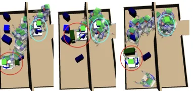
Figure 3: Key configurations that have top-10 activations for three different object placements (semi-transparent); initial configuration (cyan); final configuration (red).
Planning with the learned policy
Given a problem instance(s0, sg), we take an approach sim-ilar to (Lozano-Perez and Kaelbling 2014; Toussaint 2015) in that we try to find the continuous parameters of the plan conditioned on the given discrete plan, which is also known as aplan skeleton. The main difference is that we use the sampling-based graph search with the learned policy to guide the search.
Specifically, given a plan skeleton
{o1(δ1,·),· · ·,oT(δT,·)}, the sampling-based graph-search tries to find the continuous parameters of the operators,κ1,· · ·, κT, to make the discrete plan successful. The graph search proceeds as follows.
At the root node, the search algorithm first generatesm operator instances ofo1(δ1,·)by sampling the instances of
the parameters κ1, and adds their successor states to the
search agenda. It then pops the node from the agenda with the lowest heuristic value (estimated cost to reach the goal), and the search continues until we arrive at a goal state. If at the current node we cannot sample any feasible operators, then we discard the node and continue with the next node in the agenda. The root node is always added back to the queue after expansion, in order to guarantee completeness.
Typically, a uniform stochastic policy is used as a default choice to sample the continuous parameters, which guaran-tees probabilistic completeness. We use instead the learned policy to sample the continuous parameters.
Experiments
We evaluate ADMONin two practical and challenging G-TAMP problems, and compare against three benchmarks:
PPO,DDPG, which are actor-critic algorithms for continuous action spaces, and Generative Adversarial Imitation Learn-ing GAIL, a state-of-the-art inverse reinforcement learning algorithm that treats the planning experience dataset as op-timal demonstrations, and then uses PPO to find a policy that maximizes the learned rewards. For DDPG, we use an episodic variant that defers updates of the policy and replay buffer to the end of each episode, which makes it perform better in our inherently episodic domain. It is important to keep some level of stochasticity in any policy we learn, be-cause there is a large volume of infeasible operator instances for which no transition occurs. So, we use a Gaussian policy with a fixed variance of 0.25, and use the learned policies to predict only the mean of the Gaussian. The hyperparameters
and architectures of the actor and critic neural networks are included in the appendix.
Our hypotheses are that (a) ADMON, by using the plan-ning experience datasetDpl, can learn more data efficiently
than the benchmarks, and (b) learning these policies can im-prove planning efficiency. To test the first hypothesis, we show two plots. The first is the learning curve as a function of the size ofDpl, with a fixed number of interactions with
the simulated environment for the RL methods. For the RL methods,Dplis used as an initial training set. For ADMON,
simulations are only used for the evaluation of the current policy. For this plot, we fix the amount of RL experience at 30000 for the conveyor belt domain, and 15000 for the ob-ject fetching domain; these are obtained from 300 updates of the policy and value functions of each algorithm, where for each update, we do 5 roll-outs, each of which is 20 steps long for the first domain and 10 steps long for the second domain. We report the performance of the best policy from these 300 updates, averaged over four different random seeds. Second is the learning curve with increasing amount of simulated RL experience, with fixedDplsize. We fix its size at 100 for
the first domain and 90 for the second domain. For testing hypothesis (b), we show the improvement in planning effi-ciency when we use the best policy out of all the ones used to generate the first two plots to guide a planner.
Domain overview Our objective is to test the generaliza-tion capability of the learned policy across the changes in the poses and shapes of different number of objects in the envi-ronment, while the shape of the environment stays the same. In the first domain, the robot’s objective is to receive ei-ther four or five box-shaped objects with various sizes from a conveyor belt and pack them into a room with a narrow entrance, already containing some immovable obstacles. A problem instance is defined by the number of objects in the room, their shapes and poses, and the order of the objects that arrive on the conveyor belt. The robot must make a plan for handling all the boxes, including a grasp for each box, a placement for it in the room, and all of the robot trajectories. The initial base configuration is always fixed at the conveyor belt. After deciding the object placement, which determines the robot base configuration, a call to an RRT motion plan-ner is made to find, if possible, a collision-free path from its fixed initial configuration at the conveyor belt to the se-lected placement configuration. The robot cannot move an object once it has placed it. This is a difficult problem that involves trying a large number of infeasible motion planning problems, especially if poor sampling is used to sample con-tinuous operator parameters.
mov-able obstacles along the way, each of which involves a call to the motion planner in a relatively tight environment. We have set the problem instance distribution so that the robot must move five to eight objects to create a collision-free path to fetch the target object. This problem is a generalization of the navigation among movable obstacle problem (Stilman et al. 2007) to a mobile-manipulation setting.
In both domains, if the selected operator instance is in-feasible due to collision or kinematics, the state does not change. Otherwise, the robot picks or places the selected ob-ject with the given parameters. The reward function for the conveyor belt domain is 1 if we successfully place an object into the room and 0 otherwise. For the fetching domain, the reward function is 0 if we successfully pick an object, -1 if we try an infeasible pick or place, and 1 if we successfully move an object out of the way. For moving all the objects out of the way, the robot receives a reward of 10.
Task-level planner and sampling procedures At a high-level, the discrete operator parameters for both of the do-mains consist of the sequence of objects to be picked and placed. Specifically, two operators are given to the planner, pickandplace, each of which uses two arms to grasp a large object. Table 1 summarizes the parameters of each operator. To provide guidance, we use the policies trained with dif-ferent learning algorithms. The inputs to the policy are de-scribed in the table as well. Each operator will generally re-quire a call to a motion planner to find a collision-free path from the previous configuration.
The task-level plan for both domains is the sequence of objects to be pick-and-placed. For the conveyor domain, this is given by the problem instance definition: the objects ar-rive in the order to be packed. For the fetching domain, we implement a swept-volume approach similar to (Dogar and Srinivasa 2011; Stilman et al. 2007). We first plan a fetching motion to the target object assuming there are no movable obstacles in the scene. Then, we check the collision between this path and the moveable obstacles to identify objects that need to be moved.
To sample parameters for thepickoperation using the de-fault uniform policy:
1. Sample a collision-free base configuration,(xor, yro, ψro), uniformly from a circular region of free configuration space, with radius equal to the length of the robot’s arm, centered at the location of the object.
2. With the base configuration fixed at (xo
r, yor, ψro) from the object, sample(d, h, χ), wheredandz has a range [0.5,1], and χ has a range [π4, π], uniformly. If an in-verse kinematics (IK) solution exists for both arms for this grasp, proceed to step 3, otherwise restart.
3. Use bidirectional RRT (biRRT), or any motion planner, to get a path from the current robot base configuration to (xo
r, yor, ψro)from the pose of the object. A linear path from the current arm configuration to the IK solution found in step 2 is then planned.
If a collision is detected at any stage, the procedure restarts. When we use the learned policyπθ, we simply draw a
sam-ple from it, and then check for IK solution and path existence with the predicted grasp and base pose.
For the conveyor belt domain, we assume that the con-veyor belt drops objects into the same pose, and the robot can always reach them from its initial configuration near the conveyor belt, so we do not check for reachability. For the object fetch domain, we do all three steps.
From a state in which the robot is holding an object, it can place it at a feasible location in a particular region. To sam-ple parameters forplaceusing the default uniform policy: 1. Sample a collision-free base configuration,(x, y, ψ),
uni-formly from a desired region.
2. Use biRRT from the current robot base configuration to (x, y, ψ).
To useπθ, we sample base configurations from it in step 1. For heuristic function for the continuous-space graph search in the fetching domain, we use the number of objects to be moved out of the way as a heuristic. For the conveyor belt domain, we use the remaining number of objects to be packed as a heuristic.
To collect a datasetDpl, we use search trees constructed
while solving previous planning problems. To create a oper-ator sequenceτfrom a search tree, we begin at the root and collect state, action, and rewards up to each leaf node.
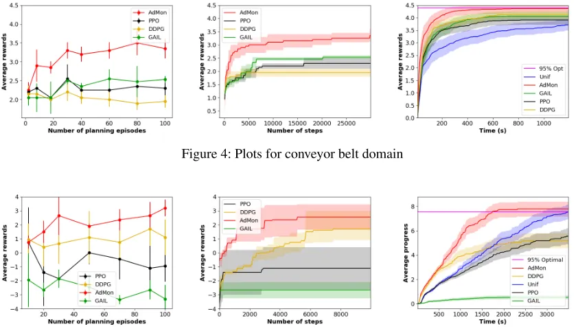
Results for the conveyor belt domain Figure 4 (left) shows the learning curve as we increase the number of search trees. Each search tree from a problem instance adds at most 50 (state, reward, operator instance, next state) tu-ples. The RL algorithms, DDPG and PPO, have rather flat learning curves. This is because they treat the planning ex-perience dataset Dpl as just another set of roll-outs; even
with 100 episodes of planning experience, this is only about 5000 transitions. Typically, these methods require tens of thousands of data to work well. ADMON, on the other hand, makes special use ofDplby trying to imitate the sequences.
On the other hand, the results fromGAILshow that it is in-effective to treatDplas optimal demonstrations and simply
do imitation. ADMON, which uses reward signals to learn a Q-function in addition to imitatingDpl, does better.
Figure 4 (middle) shows the learning curves as we in-crease the amount of transition data, while fixing the number of search trees at 100. Again, ADMONoutperforms the RL algorithms. Note that the RL approaches,DDPGandPPO, are inefficient in their use of the highly-rewardingDpl dataset.
For instance, PPO, being an on-policy algorithm, discards Dpl after an update. Even though the transition data
col-lected after that is much less informative, since it consists mostly of zero-reward transitions, it makes an update based solely on them. As a result, it tends to fall into bad local optima, and the learning curve saturates around 3000 steps. The situation is similar for the off-policy algorithmDDPG. It initially only has Dpl in its replay buffer, but as it
Operators Cont. Parameters Inputs toπθ (conv belt)
Inputs toπθ
(obj fetch)
RRT (conv belt)
RRT (obj fetch)
Pick (xo
r, yro, ψor),(d, h, χ) Learnedπθnot used φf etch, φ,(xo, yo, ψo),(l, w, h) No Yes
Place (x, y, ψ) φ φf etch, φ,(xo, yo, ψo) Yes Yes
Table 1: Operator descriptions. (x, y, ψ) refers to a robot base pose, at (x,y) location and rotationψ in the global frame, (xor, yro, ψor)refers to the relative robot base pose with respect to the pose of an object o, whose pose in global frame is (xo, yo, ψo).(d, h, χ)is a grasp represented by a depth, as a portion of size of object in the pushing direction, height, as a portion of object height, and angle in the pushing direction, respectively, and(l, w, h)represents the length, width, and height of object being picked.φf etchis a fetching path represented with key configurations. We describe this in detail in the appendix.
Figure 4: Plots for conveyor belt domain
Figure 5: Plots for object fetch domain
DDPG. It tends to escape bad local optima by learning a re-ward function that assigns high rere-wards to the planning ex-perience datasetDpl, but still performs worse than ADMON
because it treatsDplas optimal demonstrations.
Figure 4 (right) shows the reduction in planning time achieved by different learning algorithms. We can see that, after about 400 seconds, ADMON achieves 95% optimal performance, whereas the uniform policy still have not achieved that performance after 1200 seconds, indicating a speed up of at least 3.
Results for object fetch domain Figure 5 (left) shows the learning curve as we increase the number of search trees. Each search tree adds at most 50 (state, operator in-stance, next state) tuples, up to 25 of which use pick op-erator instances, and the remaining are place opop-erator in-stances. Again, the RL methods show weaker performance than ADMONalthough this time they are closer. The poor performance of GAILis due toDpl containing many more
off-target operator sequences than before, due the longer horizon. Since most of these sequences are not similar to
the solution sequence, treating these data points as optimal demonstrations hurts the learning.
Figure 5 (middle) shows the learning curve as we increase the number of transitions, while fixing the number of search trees at 90.PPOshows large variance with respect to differ-ent random seeds, and on average, shows a very steep learn-ing curve at the beginnlearn-ing, but it gets stuck at a bad local optima. DDPGshows good performance, but still performs worse than ADMON.GAILfails to learn anything meaning-ful due to the previously stated reasons.
Figure 5 (right) shows the impact on the planning effi-ciency when trained policies are used to choose the contin-uous parameters. This time, we plot the progress, measured by the number of objects cleared from the fetching path for different time limits. We can see that ADMON clears the optimal number of objects at around 1500 seconds, and the uniform policy takes 3500 seconds, an improvement in plan-ning efficiency by a factor of more than 2.3.
strat-egy used by DDPG. It is very unlikely with this strategy to encounter an episode where it clears more than 3 ob-jects. When used with the planner, which uses a heuristic, the policy starts encountering states that have more than three objects cleared, leading to poor performance. This phe-nomenon, where there is a discrepancy between the distribu-tion of states encountered during training and testing, is also noted in (Ross, Gordon, and Bagnell 2011). ADMONon the other hand does not have this problem because it is trained with the search trees produced by the planner. Note also the decrease in planning efficiency when using poor policies.
Conclusion
In this work, we proposed an actor-critic algorithm that learns from planning experience to guide a planner, us-ing key configuration features. Our experiments shows that ADMON is more data efficient than benchmarks since it uses both reward signals and the past search trees. We also demonstrated that by using the learned policy, we can achieve a substantial improvement in planning efficiency in challenging and practical G-TAMP problems.
Acknowledgement
We thank KakaoBrain for the GPU support. We grate-fully acknowledge support from NSF grants 1523767 and 1723381; from AFOSR grant FA9550-17-1-0165; from ONR grant N00014-18-1-2847; from Honda Research; and from Draper Laboratory.
References
Alami, R.; Sim´eon, T.; and Laumond, J. 1989. A geomet-rical approach to planning manipulation tasks: The case of discrete placements and grasps. International Symposium on Robotics Research.
Arjovsky, M.; Chintala, S.; and Bottou, L. 2017. Wasserstein generative adversarial networks. International Conference on Machine Learning.
Cambon, S.; Alami, R.; and Gravot, F. 2009. A hybrid ap-proach to intricate motion, manipulation, and task planning. International Journal of Robotics Research.
Dogar, M., and Srinivasa, S. 2011. A framework for push-grasping in clutter.Robotics: Science and systems.
Garrett, C. R.; Kaelbling, L. P.; and Lozano-P´erez, T. 2017. Sample-based methods for factored task and motion plan-ning. Robotics: Science and Systems.
Garrett, C. R.; Lozano-P´erez, T.; and Kaelbling, L. P. 2015. Backward-forward search for manipulation planning. IEEE/RSJ International Conference on Intelligent Robots and Systems.
Goodfellow, I.; Pouget-Abadie, J.; Mirza, M.; Xu, B.; Warde-Farley, D.; Ozair, S.; Courville, A.; and Bengio, Y. 2014. Generative adversarial nets. Advances in Neural In-formation Processing Systems.
Kaelbling, L. P., and Lozano-Perez, T. 2011. Hierarchical task and motion planning in the now. IEEE Conference on Robotics and Automation.
Kim, B.; Farahmand, A.-M.; Pineau, J.; and Precup, D. 2013. Learning from limited demonstrations. Advances in Neural Information Processing Systems.
Kim, B.; Kaelbling, L. P.; and Lozano-P´erez, T. 2017. Learning to guide task and motion planning using score-space representation.IEEE Conference on Robotics and Au-tomation.
Kim, B.; Lozano-Perez, T.; and Kaelbling, L. 2018. Guiding search in continuous state-action spaces by learning an ac-tion sampler from off-target search experience. AAAI Con-ference on Artificial Intelligence.
Konda, V. R., and Tsitsiklis, J. N. 2003. On actor-critic algorithms.SIAM Journal on Control and Optimization. Levine, S., and Abbeel, P. 2014. Learning neural network policies with guided policy search under unknown dynam-ics. Advances in Neural Information Processing Systems. Lillicrap, T. P.; J. J. Hunt, A. P.; Heess, N.; Erez, T.; Tassa, Y.; Silver, D.; and Wierstra, D. 2016. Continuous control with deep reinforcement learning.International Conference on Learning Representations.
Lozano-Perez, T., and Kaelbling, L. 2014. A constraint-based method for solving sequential manipulation planning problems.IEEE/RSJ International Conference on Intelligent Robots and Systems.
Ross, S.; Gordon, G.; and Bagnell, D. 2011. A reduction of imitation learning and structured prediction to no-regret online learning. International Conference on Artificial In-telligence and Statistics.
Schulman, J.; Wolski, F.; Dhariwal, P.; Radford, A.; and Klimov, O. 2017. Proximal policy optimization algorithms. arXiv.
Silver, D.; Huang, A.; Maddison, C.; Guez, A.; Sifre, L.; van den Driessche, G.; Schrittwieser, J.; Antonoglou, I.; Panneershelvam, V.; Lanctot, M.; Dieleman, S.; Grewe, D.; Nham, J.; Kalchbrenner, N.; Sutskever, I.; Lillicrap, T.; Leach, M.; Kavukcuoglu, K.; Graepel, T.; and Hassabis, D. 2016. Mastering the game of Go with deep neural networks and tree search. Nature.
Sim´eon, T.; Laumond, J.-P.; Cort´es, J.; and Sahbani, A. 2004. Manipulation planning with probabilistic roadmaps. International Journal of Robotics Research.
Srivastava, S.; Fang, E.; Riano, L.; Chitnis, R.; Russell, S.; and Abbeel, P. 2014. Combined task and motion planning through an extensible planner-independent interface layer. IEEE Conference on Robotics and Automation.
Stilman, M.; Schamburek, J.-U.; Kuffner, J.; and Asfour, T. 2007. Manipulation planning among movable obsta-cles. IEEE International Conference on Robotics and Au-tomation.