A Semantic Approach of ITS: Perspective on Road Safety

(1)

314 Volume-4, Issue-1, February-2014, ISSN No.: 2250-0758

International Journal of Engineering and Management Research

Available at:

www.ijemr.net

Page Number: 314-318

Inferences on Operating Characteristics of the Queue in General Earlang

Queuing System Model

P. K. Guptaand Jaideep Goel

1

Department of Statistics, D.A.V. (P.G.) College, Muzaffarnagar, (U.P.), INDIA

2_{Forest Department (U.P.), Rana Pratap Marg, Lucknow, (U.P.), INDIA}

ABSTRACT

Various queues system have been analysed in respect of their characteristics using the corresponding probability mass function (p.m.f.). Traffic intensity define as the ratio of the arrival rate to the service rate is an important concept. This ratio is also known as availability ratio in reliability theory. Various inference procedures on the queue characteristics are discussed in the present paper.

Keywords--Likelihood Estimator, UMVUE, Bayes Estimate, Prior and Posterior distribution, Queue’s characteristics

I. INTRODUCTION

In operation research problems involving queues, the investigator must measure the existing system to make an objective assessment of its characteristics and must determine how change may be made to system, what effect of various kind of change in the system characteristics would be and whether in the light of cost incurred in the system change should be made to it. In queuing theory, the traffic intensity define as the ratio of the arrival rate to the survival rate is an important concept and various queue’s characteristics are defined in [Ackoff and Sasieni (1968)] and [Taha (1976)]. In reliability theory, this ratio is also known as the availability ratio. The studies in [Mann et al. (1974)] and [Sinha (1986)] used non-bayesian and bayesian inference techniques for reliability and availability analysis in case of important life time distribution. A queue system may be better designed if the past parametric variations in the parameter of the queue system are also incorporate in the analysis of its characteristics. In addition, while recording arrival and service information over a long period of time, it seems reasonable to assume random variations in the parameter of arrival and service distribution. Thus, the objective can be met with the Bayesian analysis of various queues characteristics. In this regard, the study [Sharma and Kumar (1999)] investigate the statistical inference on

certain operating characteristics of the queue in single server M/M/1 queuing system model. Following the concept, studies like [Apostolakis (1990), Sharma and Krishna (1995), Krishna and Jain (2002), Gupta et.al. (2009)] includes the conceptual framework and methodology for such analysis.

In the present study, the maximum likelihood estimator (MLE), uniformly minimum variance unbiased estimator (UMVUE) and Bayes estimator of  and various other queue characteristics in General Earlang queuing system model have been obtained. Furthermore, testing of various estimators of performance measures has been also presented at the end of the paper to demonstrate the estimation technique applied as to showing its practical significance.

II. STATISTICAL BACKGROUND

(a) The p.m.f. of a General Earlang queue system with poission input and poission out is

!

x

e

P

x





 ;x=0 1, 2 …(1) (1)

Here,

(i) Px : The probability that at any time there are x units in

the queue. Thus, the random variable x follow a Poission distribution with parameter



.

(ii)  : The traffic intensity or service factor.

(b) Based on p.m.f. in (1), various important characteristics of the queue system are

(i) Ls =  : Expected queue length

(ii) Lq = +e--1 : Expected length of waiting line

(iii) Qm= P [x >no]

x

!

p

e

x

o n

0 x

 







:The probability of minimum

queue size being no

(2)

315

= 1- e- :Utilization of the server

III. ASSUMPTIONS

(a) Let there be k identical and independent queue system. Also there are xi units in the ith system at any given time

point (i = 1, 2,…, k)

(b) For Bayesian analysis, the investigator’s prior belief about  is assumed to be gamma distribution with p.d.f.

1

.

e

.

)!

1 (

)

,

(

g





















; , > 0 … (2)

with mean = / and variance = /2_.

IV. INFERENCES ON OPERATING

QUEUE CHARACTERISTICS

(a) MLE’s

As assumed at any given time, there are xi units

in the ith system (i = 1, 2, …, k). Therefore, the joint p.m.f. of x1, x2, …, xk is given by

!

x

!...

x

!

x

.

e

)

;

x

...

,

x

,

(x

g

k 2 1

y k

-k 2 1







 …(3)

where  



k 1 i

x

i

y

.

Now





log [g (x1, x2, …, xk; )] = 0 gives the M.L.E. of

, say



ˆ

as

k

/

y

ˆ





…(4) On using invariance property of MLE’s (i) The MLE of Ls, i.e.

L

ˆ

_s is

L

ˆ

s





ˆ



y/k

…(5) (ii) Similarly, the MLE of Lq, i.e.

L

ˆ

q

L

ˆ

e

1 ˆ

ˆ

q











1 e

k

y

_y_/_k









…(6)

(iii) The MLE of Qm i.e.

Q

ˆ

_m will be

! x

) k / y .( e 1

! x

) ˆ .( e 1

Qˆ

x k / y 1 o n

0 x x

ˆ 1 o n

0 x m

 

 

 

   

 

 

…(7)

(iv) Finally, the MLE for  say



ˆ

will be

 







ˆ

1 e

ˆ



1ey/k …(8)

(b) UMVUE’s

According to Rao-Blackwell-Lehmann-Scheffe’s theorem [Rohatgi (1985)], If T is a complete sufficient statistics and there exists an unbiased estimate h of , there exists a unique UMVUE of , which is given by E [h/T].In our case, the well known factorization

method shows that the statistics





 k

1 i

i

x

y

is a sufficient

statistics for . Also, the family of the distribution of y, i.e. Poission () is known to be complete [Rohatgi (1986)].

y!

)

k

.(

e

y]

[Y

P

y

k

_



  ; y = 0, 1, 2.. …(9) (9)

Also in Poission distribution, we haveE [y(r)] = (k)r

i.e. r

r ) r (

k

y

E

















Thus, r

) r (

k

y

is an unbiased estimator of r. Also it is a

function of complete sufficient statistics, so by

Lehmann-Scheffe’s theorem r

) r (

k

y

is the UMVUE of r. Taking

r=1, we get the UMVUE of  i.e.

k

y

~

_



…(10)

Further, since Ls = , hence the UMVUE of Ls say

L

_s

~

is same as the UMVUE of , i.e.

k

y

~

L

~

_s







…(11) For < 1, to obtain the UMVUE of Lq, we define











otherwise

:

0

0 x

if

:

1 )

x

(

1

 











(

x

)]

1 .

P

(x

0)

0. P

(x

0)

e

[

E

₁ ₁

It’s mean,(x) is an unbiased estimator for e-_.

Thus by Lehmann-Scheffe’s theorem, E[(x)| y = y] is the UMVUE for e- Thus,

y]

y

|

0 [x

P

]

y

|

)

x

(

[

E





₁



y

i k

1 i

i k

2 i 1

k

1

1 y

x

P

y

x

P

)

0 x

(

P



















































(3)

316

which is a function of complete sufficient statistics. Thus, it is the UMVUE of e. On using (10),

(12) and [Rohatgi (1985) p. 354], the UMVUE for Lq say

q

L

~

becomes as

1 k

1

1 k

y

L

~

y

q





















…(13)

Similarly, for obtaining the UMVUE of the Qm, we

consider a function (X) such that











otherwise

:

0 k

x

if

:

1 )

x

(

1

E[(x)] = 1. P (x1 =k) + 0. P(x1 k) =

!

k

.

e





k

Thus, (x) is an unbiased estimator of

!

k

.

e





k

. Also it

is a function of complete sufficient statistics, so E [(x)| Y

= y] is the UMVUE for

!

k

P

.

e

 k

. Therefore























































  

y

x

P

y

x

k

x

P

x

Y

)

x

(

E

n 1 i i k 2 i i 1 k 1 i i n y n

k

1

1 .

k

1 .

n

y











































…(14)

On using (14) and [Rohatgi (1985), p.354], one gets the UMVUE for Qm i.e.

u y u 1 o n o u m

k

1

1 .

k

1 .

u

y

1 Q

~

  













































…(15)

Finally, for obtaining the UMVUE of , we used equation (12) and [Rohatgi (1985), p. 354], the UMVUE of  say



~

_is

y

k

1

1 ~



















…(16)

(c) Bayesian Estimation

For Bayes estimation of queues characteristics, let us regard  as a random variable with prior distribution defined in (2). Suppose

x

(

x

₁

,

x

₂

,...,

x

_k

)

~



be a random

sample taken from the population (1), then the joint distribution of  and the sample can be written as

1 k 2 1 k 1 i i x n

~

x

!

x

!...

x

!

(

1 )!

.

e

.

e

)

(

g

).

x

(

L

 

    















consider  



k 1 i

x

i

y

, the posterior distribution of , becomes 1 y ) k ( y

~ (y 1)!.e . ) k ( x /              _      

 …(17)

The posterior distribution of  in (17) is the well known gamma distribution with parameters (k + ) and (y + ).

Having obtained the posterior distribution of  in (17), the Bayes point estimator  say * can be defined as           





_

 .e  .  .d )! 1 y ( ) k ( . ] x | [

E (k ) y -1

y

~ *

o

(

k

)

y

(











…(18)

Further, for < 1, the Bayes estimator of Ls, say

* s

L

is

)

k

(

)

(y

]

x

|

L

[

E

L

~ s *

s

_

_







…(19)

Similarly, for < 1, the Bayes estimator of Lq, say

* q

L

is

1 ) 1 k ( ) k ( ) k ( ) (y ] x | L [ E L y y ~ q * q              __ …(20)

Also, for < 1, the Bayes estimator of Qm is

] ~ x | Q [ E Q*_m _m

                              __ 2 y y ) 1 k .( 2 ) 1 y )( y ( ) 1 k ( ) y ( 1 ) 1 k ( ) k ( 1 …(21) Finally, the Bayes estimator for  is

]

~

x

|

[

E

*

_

_



  















y y

)

1 k

(

)

k

(

1

…. (22)

V. DISCUSSION AND EXAMPLE

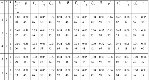
MLE’s for , Ls, Lq, Qm and  are given in

subsection 4 (a). Their corresponding UMVUE’s are obtained in subsection 4 (b). Bayes estimators for these all queues characteristics are obtained in equations (18-22). For analysing the behaviour of these MLE’s, UMVUE’s and Bayes estimators of various queues characteristics, keeping some of the parameters fixed and varying others. On taking k = 13, y = 5,  = 2, no= 3 and varying [or

(4)

317

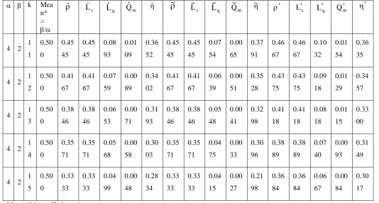
estimators are shown in Table 1. Trends in Table-1 clearly reveals that MLE’s and UMVUE’s of all the queue’s characteristics are constant while Bayes estimates of all the characteristics tends to be decreases as mean of the traffic intensity decrease. In yet another example on assuming  = 2,  = 4, y = 5, no = 3 and varying k [the number of the

system], the trends in various characteristics are summarized in Table -2. Trends in Table-2 highlighted that MLE’s, UMVUE’s and Bayes estimators of all the characteristics tend to be decreased as k increases. Following this pattern, the behavior of all these characteristics with respect to variations in other parameters can be studied, measured and interpreted.

REFERENCES

[1] Ackoff, R.L. and Sasieni, M.W. (1968), “Fundamental of Operations Research”, Wiley Eastern Limited, New York.

[2] Apostolakis, G. (1990), “The Concept of Probability in Safety Assessment of Technological System”, Science, 250, 139-146.

[3] Krishna, H. and Jain, N. (2002), “Classical and Bayes Estimation of Reliability Characteristics of Some System Configurations with Geometric Lifetimes of Components”, IAPQR Transaction, Calcutta, 27 (1).

[4] Mann, N.R., Schafer, R.E. and Singpurwala (1974), “Methods for Statistical Analysis of Reliability and Lifetime Data”, John Wiley and Sons, New York.

[5] P. K. Gupta, Jaideep Goel and R. Kumar(2009), “Posteriror Analysis of The Queue Characteristics in Power Supply System Model”Bulle. Of Allahabad Mathematical Society, Vol.-24, part-2, pp.297-306. [6] Rohatgi, V.K. (1985), “An Introduction to Probability Theory and Mathematical Statistics”, John Wiley and Sons.

[7] Sharma, K.K. and Krishna, H. (1995), “Bayes Estimates of Pointwise and Internal Availability with Type I Censored Samples”, Microelectron Reliab., 35 (1), 33-36. [8] Sharma, K.K. and Kumar, V. (1999), “Inferences on M/M/1: (/FIFO) Queue System”, Opsearch, 36, 1, 26-34. [9] Sinha, S.K. (1986), “Reliability and Life Testing”, Wiley Eastern Limited, New York.

[10] Taha, H.A. (1976), “Operation Research – An Introduction”, Macmillan, New York.

Table 1

Estimates of queue’s characteristics with variations in mean traffic intensity

  k Mea n* = /



ˆ

_L

ˆ

_s q

L

ˆ

Q

ˆ

m



ˆ



~

s

L

~

q

L

~

m

Q

~



~



*

L

*s *

q

L

Q

*m



*

2 2 1 3

1.00

00

0.38

46

0.38

46

0.06

53

0.05

42

0.31

93

0.38

46

0.38

46

0.05

48

0.00

42

0.32

97

0.46

67

0.46

67

0.10

32

0.01

54

0.36

35

3 2 1 3

0.66

67

0.38

46

0.38

46

0.06

53

0.05

42

0.31

93

0.38

46

0.38

46

0.05

48

0.00

42

0.32

97

0.43

75

0.43

75

0.09

18

0.01

29

0.34

57

4 2 1 3

0.50

00

0.38

46

0.38

46

0.06

53

0.05

42

0.31

93

0.38

46

0.38

46

0.05

48

0.00

42

0.32

97

0.41

18

0.41

18

0.08

18

0.01

15

0.33

00

5 2 1 3

0.40

00

0.38

46

0.38

46

0.06

53

0.05

42

0.31

93

0.38

46

0.38

46

0.05

48

0.00

42

0.32

97

0.38

89

0.38

89

0.07

40

0.00

93

0.31

49

6 2 1 3

0.33

33

0.38

46

0.38

46

0.06

53

0.05

42

0.31

93

0.38

46

0.38

46

0.05

48

0.00

42

0.32

97

0.36

84

0.36

84

0.06

67

0.00

84

0.30

17

(5)

318

Table 2

Estimates of queue’s characteristics with variations in k

  k Mea n* = /



ˆ

L

ˆ

_s

L

ˆ

_q

Q

ˆ

m



ˆ



~

s

L

~

q

L

~

m

Q

~



~



*

L

*_s

L

*_q

Q

*m



*

4 2 1 1

0.50

0

0.45

45

0.45

45

0.08

93

0.01

09

0.36

52

0.45

45

0.45

45

0.07

54

0.00

65

0.37

91

0.46

67

0.46

67

0.10

32

0.01

54

0.36

35

4 2 1 2

0.50

0

0.41

67

0.41

67

0.07

59

0.00

89

0.34

02

0.41

67

0.41

67

0.06

39

0.00

51

0.35

28

0.43

75

0.43

75

0.09

18

0.01

29

0.34

57

4 2 1 3

0.50

0

0.38

46

0.38

46

0.06

53

0.00

71

0.31

93

0.38

46

0.38

46

0.05

48

0.00

41

0.32

98

0.41

18

0.41

18

0.08

18

0.01

15

0.33

00

4 2 1 4

0.50

0

0.35

71

0.35

71

0.05

68

0.00

58

0.30

03

0.35

71

0.35

71

0.04

75

0.00

33

0.30

96

0.38

89

0.38

89

0.07

40

0.00

93

0.31

49

4 2 1 5

0.50

0

0.33

33

0.33

33

0.04

99

0.00

48

0.28

34

0.33

33

0.33

33

0.04

15

0.00

27

0.21

98

0.36

84

0.36

84

0.06

67

0.00

84

0.30

17