A Constructive Approach to
L
0Penalized Regression
Jian Huang [email protected]
Department of Applied Mathematics The Hong Kong Polytechnic University Hung Hom, Kowloon
Hong Kong, China
Yuling Jiao∗ [email protected]
School of Statistics and Mathematics Zhongnan University of Economics and Law Wuhan, 430063, China
Yanyan Liu [email protected]
School of Mathematics and Statistics Wuhan University
Wuhan, 430072, China
Xiliang Lu† [email protected]
School of Mathematics and Statistics Wuhan University
Wuhan, 430072, China
Editor:Tong Zhang
Abstract
We propose a constructive approach to estimating sparse, high-dimensional linear regression models. The approach is a computational algorithm motivated from the KKT conditions for the`0-penalized least squares solutions. It generates a sequence of solutions iteratively,
based on support detection using primal and dual information and root finding. We refer to the algorithm as SDAR for brevity. Under a sparse Riesz condition on the design matrix and certain other conditions, we show that with high probability, the`2 estimation error
of the solution sequence decays exponentially to the minimax error bound inO(log(R√J)) iterations, whereJ is the number of important predictors andR is the relative magnitude of the nonzero target coefficients; and under a mutual coherence condition and certain other conditions, the`∞ estimation error decays to the optimal error bound inO(log(R))
iterations. Moreover the SDAR solution recovers the oracle least squares estimator within a finite number of iterations with high probability if the sparsity level is known. Com-putational complexity analysis shows that the cost of SDAR is O(np) per iteration. We also consider an adaptive version of SDAR for use in practical applications where the true sparsity level is unknown. Simulation studies demonstrate that SDAR outperforms Lasso, MCP and two greedy methods in accuracy and efficiency.
Keywords: Geometrical convergence, KKT conditions, nonasymptotic error bounds, oracle property, root finding, support detection
∗. Also in the Institute of Big Data of Zhongnan University of Economics and Law
†. Also in the Hubei Key Laboratory of Computational Science
c
1. Introduction
Consider the linear regression model
y =Xβ∗+η (1)
where y ∈ Rn is a response vector, X ∈
Rn×p is the design matrix with
√
n-normalized
columns,β∗= (β1∗, . . . , βp∗)0 ∈Rp is the vector of the underlying regression coefficients and
η ∈Rn is a vector of random noises. We focus on the case where p n and the model is
sparse in the sense that only a relatively small number of predictors are important. Without
any constraints on β∗ there exist infinitely many least squares solutions for (1) since it is
a highly undetermined linear system when p n. These solutions usually over-fit the
data. Under the assumption that β∗ is sparse in the sense that the number of important
nonzero elements ofβ∗ is small relative to n, we can estimate β∗ by the solution of the `0
minimization problem
min β∈Rp
1
2nkXβ−yk
2
2, subject to kβk0≤s, (2)
wheres >0 controls the sparsity level. However, (2) is generally NP hard (Natarajan, 1995;
Chen et al., 2014), hence it is not tractable to design a stable and fast algorithm to solve it, especially in high-dimensional settings.
In this paper we propose a constructive approach to approximating the `0-penalized
solution to (1). The approach is a computational algorithm motivated from the necessary KKT conditions for the Lagrangian form of (2). It finds an approximate sequence of solu-tions to the KKT equasolu-tions iteratively based on support detection and root finding until convergence is achieved. For brevity, we refer to the proposed approach as SDAR.
1.1 Literature review
Several approaches have been proposed to approximate (2). Among them the Lasso
(Tib-shirani, 1996; Chen et al., 1998), which uses the `1 norm of β in the constraint instead of
the`0 norm in (2), is a popular method. Under the irrepresentable condition on the design
matrix X and a sparsity assumption on β∗, Lasso is model selection (and sign) consistent
(Meinshausen and B¨uhlmann, 2006; Zhao and Yu, 2006; Wainwright, 2009). Lasso is a
con-vex minimization problem. Several fast algorithms have been proposed, including LARS (Homotopy) (Osborne et al., 2000; Efron et al., 2004; Donoho and Tsaig, 2008), coordinate descent (Fu, 1998; Friedman et al., 2007; Wu and Lange, 2008), and proximal gradient descent (Agarwal et al., 2012; Xiao and Zhang, 2013; Nesterov, 2013).
However, Lasso tends to overshrink large coefficients, which leads to biased estimates (Fan and Li, 2001; Fan and Peng, 2004). The adaptive Lasso proposed by Zou (2006) and analyzed by Huang et al. (2008b) in high-dimensions can achieve the oracle property under certain conditions, but its requirements on the minimum value of the nonzero coefficients are not optimal. Nonconvex penalties such as the smoothly clipped absolute deviation (SCAD) penalty (Fan and Li, 2001), the minimax concave penalty (MCP) (Zhang, 2010a)
and the capped `1 penalty (Zhang, 2010b) were proposed to remedy these problems (but
Although the global minimizers (also certain local minimizers) of these nonconvex regular-ized models can eliminate the estimation bias and enjoy the oracle property (Zhang and Zhang, 2012), computing the global or local minimizers with the desired statistical proper-ties is challenging, since the optimization problem is nonconvex, nonsmooth and large scale in general.
There are several numerical algorithms for nonconvex regularized problems. The first kind of such methods can be considered a special case (or variant) of minimization maxi-mization algorithm (Lange et al., 2000; Hunter and Li, 2005) or of multi-stage convex relax-ation (Zhang, 2010b). Examples include local quadratic approximrelax-ation (LQA) (Fan and Li, 2001), local linear approximation (LLA) (Zou and Li, 2008), decomposing the penalty into a difference of two convex terms (CCCP) (Kim et al., 2008; Gasso et al., 2009). The second type of methods is the coordinate descent algorithms, including coordinate descent of the Gauss-Seidel version (Breheny and Huang, 2011; Mazumder et al., 2011) and coordinate descent of the Jacobian version, i.e., the iterative thresholding method (Blumensath and Davies, 2008; She, 2009). These algorithms generate a sequence of solutions at which the objective functions are nonincreasing, but the convergence of the sequence itself is generally unknown. Moreover, if the sequence generated from multi-stage convex relaxation (starts from a Lasso solution) converges, it converges to some stationary point which may enjoy certain oracle statistical properties with the cost of a Lasso solver per iteration (Zhang, 2010b; Fan et al., 2014). Huang et al. (2018) proposed a globally convergent primal dual active set algorithm for a class of nonconvex regularized problems. Recently, there has been much effort to show that CCCP, LLA and the path following proximal-gradient method can track the local minimizers with the desired statistical properties (Wang et al., 2013; Fan et al., 2014; Wang et al., 2014; Loh and Wainwright, 2015).
Another line of research concerns the greedy methods such as the orthogonal matching pursuit (OMP) (Mallat and Zhang, 1993) for solving (2) approximately. The main idea is to iteratively select one variable with the strongest correlation with the current residual at a time. Roughly speaking, the performance of OMP can be guaranteed if the small
subma-trices ofX are well conditioned like orthogonal matrices (Tropp, 2004; Donoho et al., 2006;
Cai and Wang, 2011; Zhang, 2011b). Fan and Lv (2008) proposed a marginal correlation learning method called sure independence screening (SIS), see also Huang et al. (2008a) for an equivalent formulation that uses penalized univariate regression for screening. Fan and Lv (2008) recommended an iterative SIS to improve the finite-sample performance. As they discussed the iterative SIS also uses the core idea of OMP but it can select more features at each iteration. There are several more recently developed greedy methods aimed at selecting several variables a time or removing variables adaptively, such as iterative hard thresholding (IHT) (Blumensath and Davies, 2009; Jain et al., 2014) or hard thresholding gradient de-scent (GraDes) (Garg and Khandekar, 2009), adaptive forward-backward selection (FoBa) (Zhang, 2011a).
Liu and Wu (2007) proposed a Mixed Integer Optimization (MIO) approach for solving
penalized classification and regression problems with a penalty that is a combination of`0
and `1 penalties. However, they only considered low-dimensional problems with p in the
10s andnin the 100s. Bertsimas et al. (2016) also considered an MIO approach for solving
min-utes, for example, for (n, p)≈(100,1000) or (n, p)≈(1000,100). For the p > nexamples, the authors carried out all the computations on Columbia University’s high performance
computing facility using a commercial MIO solver Gurobi (Gurobi Optimization, 2015).
In comparison, our proposed approach can deal with high-dimensional models. For the
examples we consider in our simulation studies with (n, p) = (5000,50000), it can find the
solution in seconds on a personal laptop computer.
1.2 Contributions
SDAR is a new approach for fitting sparse, high-dimensional regression models. Compared
with the penalized methods, SDAR generates a sequence of solutions {βk, k ≥ 1} to the
KKT system of the `0 penalized criterion, which can be viewed as a primal-dual active set
method for solving the `0 regularized least squares problem with a changing regularization
parameterλin each iteration (this will be explained in detail in Section 2).
We show that SDAR achieves sharp estimation error bounds within a finite number of
iterations. Specifically, we show that: (a) under a sparse Riesz condition onXand a sparsity
assumption onβ∗,kβk−β∗k2achieves the minimax error bound up to a constant factor with
high probability inO(√Jlog(R)) iterations, whereJ is the number of important predictors
andRis the relative magnitude of the nonzero target coefficients (the exact definitions ofJ
andR are given in Section 3); (b) under a mutual coherence condition onX and a sparsity
assumption on β∗, the kβk −β∗k∞ achieves the optimal error bound O(σp
log(p)/n) in
O(log(R)) iterations; (c) under the conditions in (a) and (b), with high probability, βk
coincides with the oracle least squares estimator inO(√Jlog(R)) andO(log(R)) iterations,
respectively, ifJ is available and the minimum magnitude of the nonzero elements of β∗ is
of the order O(σp2 log(p)/n),which is the optimal magnitude of detectable signal.
An interesting aspect of the result in (b) is that the number of iterations for SDAR to
achieve the optimal error bound is O(log(R)), which does not depend on the underlying
sparsity level. This is an appealing feature for the problems with a large triple (n, p, J).
We also analyze the computational cost of SDAR and show that it is O(np) per iteration,
comparable to the existing penalized methods and the greedy methods. In summary, the main contributions of this paper are as follows.
• We propose a new approach to fitting sparse, high-dimensional regression models.
The approach seeks to directly approximate the solutions to the KKT equations for
the`0 penalized problem.
• We show that the sequence of solutions{βk, k≥1} generated by the SDAR achieves
sharp error bounds within a finite number of iterations.
• We also consider an adaptive version of SDAR, or simply ASDAR, by tuning the
1.3 Notation
For a column vectorβ= (β1, . . . , βp)0∈Rp, denote itsq-norm bykβkq= (Ppi=1|βi|q)1/q, q∈
[1,∞],and its number of nonzero elements bykβk0. Let0denote a column vector inRpor a
matrix whose elements are all 0. LetS={1,2, ..., p}. For anyAandB ⊆S with length|A|
and |B|, let βA= (βi, i∈A)∈R|A|, XA= (Xi, i∈A)∈Rn×|A|,and letXAB ∈R|A|×|B| be
a submatrix ofX whose rows and columns are listed inAandB,respectively. Letβ|A∈Rp
be a vector with itsi-th element (β|A)i =βi1(i∈A), where1(·) is the indicator function.
Denote the support of β by supp(β). Denote A∗ = supp(β∗) and K =kβ∗k0. Let kβkk,∞
and |β|min be thekth largest elements (in absolute value) and the minimum absolute value
of β, respectively. Denote the operator norm of X induced by the vector 2-norm bykXk.
LetI be an identity matrix.
1.4 Organization
In Section 2 we develop the SDAR algorithm based on the necessary conditions for the `0
penalized solutions. In Section 3 we establish the nonasymptotic error bounds of the SDAR solutions. In Section 4 we describe the adaptive SDAR, or ASDAR. In Section 5 we analyze the computational complexity of SDAR and ASDAR. In Section 6 we compare SDAR with several greedy methods and a screening method. In Section 7 we conduct simulation studies to evaluate the performance of SDAR/ASDAR and compare it with Lasso, MCP, FoBa and DesGras. We conclude in Section 8 with some final remarks. The proofs are given in the Appendix.
2. Derivation of SDAR
Consider the Lagrangian form of the `0 regularized minimization problem (2),
min β∈Rp
1
2nkXβ−yk
2
2+λkβk0. (3)
Lemma 1 Let β be a coordinate-wise minimizer of (3). Thenβ satisfies:
(
d=X0(y−Xβ)/n, β =Hλ(β+d),
(4)
where Hλ(·) is the hard thresholding operator defined by
(Hλ(β))i = (
0, if |βi|<
√
2λ, βi, if |βi| ≥
√
2λ. (5)
Conversely, if β and d satisfy (4), then β is a local minimizer of (3).
Remark 2 Lemma 1 gives the KKT condition of the `0 regularized minimization problem (3), which is also derived in Jiao et al. (2015). Similar results for SCAD, MCP and
Let A = supp(β) and I = (A)c. Suppose that the rank of XA is |A|. From the
definition ofHλ(·) and (4) it follows that
A = n
i∈S|βi +di| ≥
√
2λ
o
, I = n
i∈S|βi+di|<
√
2λ
o
,
and
βI=0, dA=0,
βA= (XA0XA)−1X0 Ay, dI=XI0(y−XAβ
A)/n.
We solve this system of equations iteratively. Let {βk, dk} be the solution at the kth
iteration. We approximate {A, I} by
Ak= n
i∈S|βik+dki| ≥
√
2λ
o
, Ik= (Ak)c. (6)
Then we can obtain an updated approximation pair{βk+1, dk+1} by
βkIk+1 =0,
dkA+1k =0,
βkA+1k = (X 0
AkXAk)−1XA0ky,
dkI+1k =X 0
Ik(y−XAkβk+1
Ak )/n.
(7)
Now suppose we want the support of the solutions to have the size T, where T ≥ 1 is a
given integer. We can choose
√
2λk,kβk+dkk
T ,∞ (8)
in (6). With this choice of λ, we have |Ak|=T, k ≥1. Then with an initial β0 and using
(6) and (7) with theλk in (8), we obtain a sequence of solutions{βk, k≥1}.
There are two key aspects of SDAR. In (6) we detect the support of the solution based
on the sum of the primal (βk) and dual (dk) approximations and, in (7) we calculate the
least squares solution on the detected support. Therefore, SDAR can be considered an iterative method for solving the KKT equations (4) with an important modification: a
different λ value given in (8) in each step of the iteration is used. Thus we can also view
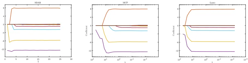
0 5 10 15 20 25 30 T -12 -8 -4 0 4 8 C o e ffi c ie n t SDAR 10-2 10-1 100 101 102 λ -12 -8 -4 0 4 8 C o e ffi c ie n t MCP 10-3 10-2 10-1 100 101 102 λ -12 -8 -4 0 4 8 C o e ffi c ie n t Lasso
Figure 1: The solution paths of SDAR, MCP and Lasso. We see that large components
were selected in by SDAR gradually when T increases. This is similar to Lasso
and MCP asλdecreases.
As an example, Figure 1 shows the solution path of SDAR with T = 1,2, . . . ,5K along
with the MCP and the Lasso paths on 5K different λvalues for a data set generated from
a model with (n = 50, p= 100, K = 5, σ = 0.3, ρ = 0.5, R = 10), which will be described
in Section 7. The Lasso path is computed using LARS (Efron et al., 2004). Note that
the SDAR path is a function of the fitted model size T = 1, . . . , L, where L is the size
of the largest fitted model. In comparison, the paths of MCP and Lasso are functions of
the penalty parameter λ in a prespecified interval. In this example, when T ≤ K, SDAR
selects the firstT largest components of β∗ correctly. When T > K, there will be spurious
elements included in the estimated support, the exact number of such elements is T −K.
In Figure 1, the estimated coefficients of the spurious elements are close to zero.
Algorithm 1 Support detection and root finding (SDAR)
Require: β0,d0 =X0(y−Xβ0)/n,T; set k= 0.
1: fork= 0,1,2,· · · do
2: Ak ={i∈S|βik+dik| ≥ kβk+dkkT ,∞}, Ik= (Ak)c
3: βIkk+1 =0 4: dkA+1k =0 5: βAk+1k = (X
0
AkXAk)−1X0
Aky 6: dkIk+1=X
0
Ik(y−XAkβk+1
Ak )/n 7: if Ak+1=Ak,then
8: Stop and denote the last iteration byβAˆ, βIˆ, dAˆ, dIˆ
9: else
10: k=k+ 1
11: end if
12: end for Ensure: βˆ= (β0ˆ
A, β
0 ˆ
I)
0 as the estimate ofβ∗.
Remark 3 IfAk+1 =Ak for somekwe stop SDAR since the sequences generated by SDAR will not change. Under certain conditions, we will show that Ak+1 = Ak =supp(β∗) if k
3. Nonasymptotic error bounds
In this section we present the nonasymptotic `2 and `∞ error bounds for the solution
sequence generated by SDAR as given in Algorithm 1.
We say that X satisfies the sparse Rieze condition (SRC) (Zhang and Huang, 2008;
Zhang, 2010a) with ordersand spectrum bounds {c−(s), c+(s)} if
0< c−(s)≤
kXAuk22
nkuk22 ≤c+(s)<∞,∀06=u∈R
|A| withA⊂S and |A| ≤s.
We denote this condition by X ∼ SRC{s, c−(s), c+(s)}. The SRC gives the range of the
spectrum of the diagonal sub-matrices of the Gram matrixG =X0X/n. The spectrum of
the off diagonal sub-matrices ofGcan be bounded by the sparse orthogonality constantθa,b
defined as the smallest number such that
θa,b≥
kXA0 XBuk2
nkuk2 ,∀06=u∈R
|B| withA, B ⊂S,|A| ≤a,|B| ≤b, and A∩B=∅.
Another useful quantity is the mutual coherenceµdefined asµ= maxi6=j|Gi,j|, which
char-acterizes the minimum angle between different columns of X/√n. Some useful properties
of these quantities are summarized in Lemma 20 in the Appendix.
In addition to the regularity conditions on the design matrix, another key condition is the
sparsity of the regression parameter β∗. The usual sparsity condition is to assume that the
regression parameterβ∗i is either nonzero or zero and that the number of nonzero coefficients
is relatively small. This strict sparsity condition is not realistic in many problems. Here
we allow that β∗ may not be strictly sparse but most of its elements are small. Let A∗J =
{i∈ S :|βi∗| ≥ kβ∗kJ,∞} be the set of the indices of the first J largest components of β∗.
Typically, we haveJ n. Let
R= ¯
M
¯
m, (9)
where ¯m= min{|βi∗|, i∈A∗J} and ¯M = max{|βi∗|, i∈A∗J}. Since β∗=β∗|A∗
J +β ∗|
(A∗
J)c, we
can transform the non-exactly sparse model (1) to the following exactly sparse model by
including the small components of β∗ in the noise,
y=Xβ¯∗+ ¯η, (10)
where
¯
β∗=β∗|A∗
J and ¯η =Xβ
∗|
(A∗J)c+η. (11)
Let RJ =kβ∗|(A∗
J)ck2+kβ ∗|
(A∗
J)ck1/ √
J, which is a measure of the magnitude of the small
components of β∗ outside A∗J. Of course, RJ = 0 if β∗ is exactly K-sparse with K ≤ J.
Without loss of generality, we letJ =K,m= ¯mandM = ¯M for simplicity ifβ∗ is exactly
K-sparse.
LetβJ,obe the oracle estimator defined asβJ,o = arg minβ{21nky−Xβk22, βj = 0, j 6∈A∗J},
that is, βAJ,o∗
J = X †
A∗Jy and β J,o
(A∗
J)c
= 0, where XA†∗
J is the generalized inverse of XA
∗
J and
equals to (XA0∗
JXA
∗
J) −1X0
A∗
J ifXA
∗
J is of full column rank. Soβ
J,o is obtained by keeping the
predictors corresponding to theJ largest components of β∗ in the model and dropping the
other predictors. Obviously,βJ,o =βoifβ∗is exactlyK-sparse, whereβAo∗ =X
†
3.1 `2 error bounds
Let 1 ≤ T ≤ p be a given integer used in Algorithm 1. We require the following basic
assumptions on the design matrixX and the error vectorη.
(A1) The input integerT used in Algorithm 1 satisfiesT ≥J.
(A2) For the input integerT used in Algorithm 1,X∼SRC{2T, c−(2T), c+(2T)}.
(A3) The random errors η1, . . . , ηn are independent and identically distributed with
mean zero and sub-Gaussian tails, that is, there exists a σ ≥ 0 such that E[exp(tηi)] ≤
exp(σ2t2/2) fort∈
R1,i= 1, . . . , n.
Let
γ = 2θT ,T + (1 +
√
2)θ2T,T c−(T)2
+(1 +
√
2)θT ,T
c−(T)
.
Define
h2(T) = max
A⊆S:|A|≤TkX
0
Aη¯k2/n, (12)
where ¯η is defined in (11).
Theorem 4 Let T be the input integer used in Algorithm 1, where 1 ≤ T ≤ p. Suppose
γ <1.
(i) Assume (A1) and (A2) hold. We have
kβ¯∗|A∗
J\Ak+1k2≤γ
k+1kβ¯∗k 2+
γ
(1−γ)θT ,T
h2(T), (13)
kβk+1−β¯∗k2≤b1γkkβ¯∗k2+b2h2(T), (14) where
b1 = 1 +
θT,T
c−(T)
and b2 =
γ
(1−γ)θT ,T
b1+
1
c−(T)
. (15)
(ii) Assume (A1)-(A3) hold. Then for any α ∈(0,1/2), with probability at least 1−2α,
kβ¯∗|A∗
J\Ak+1k2 ≤γ
k+1kβ¯∗k 2+
γ
(1−γ)θT,T
ε1, (16)
kβk+1−β¯∗k2 ≤b1γkkβ¯∗k2+b2ε1, (17) where
ε1=c+(J)RJ +σ
√
Tp2 log(p/α)/n. (18)
Remark 6 Assumption (A1) is necessary for SDAR to select at least J nonzero features. The SRC in (A2) has been used in the analysis of the Lasso and MCP (Zhang and Huang, 2008; Zhang, 2010a). Sufficient conditions are provided for a design matrix to satisfy the SRC in Propositions 4.1 and 4.2 in Zhang and Huang (2008). For example, the SRC would follow from a mutual coherence condition. Let c(T) = (1−c−(2T))∨(c+(2T)−1), which is closely related to the the RIP (restricted isometry property) constant δ2T for X (Candes
and Tao, 2005). By (43) in the Appendix, it can be verified that a sufficient condition for γ < 1 is c(T) ≤ 0.1599, i.e., c+(2T) ≤ 1.1599, c−(2T) ≥ 0.8401. The sub-Gaussian condition (A3) is often assumed in the literature on sparse estimation and slightly weaker than the standard normality assumption. It is used to calculate the tail probabilities of certain maximal functions of the noise vector η.
Remark 7 Several greedy algorithms have also been studied under the assumptions related to the sparse Riesz condition. For example, Zhang (2011b) studied OMP under the condition
c+(T)/c−(31T)≤2. Zhang (2011a) analyzed the forward-backward greedy algorithm (FoBa) under the condition8(T+ 1)≤(s−2)T c2−(sT), wheres >0is a properly chosen parameter. GraDes has been analyzed under the RIP conditionδ2T ≤1/3 (Garg and Khandekar, 2009).
These conditions and (A2) are related but do not imply each other. The order of `2-norm estimation error of SDAR is at least as good as that of the above mentioned greedy methods since it achieves the minimax error bound, see, Remark 10 below. A high level comparison between SDAR and the greedy algorithms will be given in Section 6.
Corollary 8 (i) Suppose (A1) and (A2) hold. Then
kβk−β¯∗k2 ≤ch2(T) if k≥log1
γ √
JM¯ h2(T)
, (19)
where c=b1+b2 with b1 andb2 defined in (15). Furthermore, assume m¯ ≥ γh2(T)
(1−γ)θT ,Tξ for some 0< ξ <1, then we have
Ak ⊇A∗J if k≥log1
γ √
J R
1−ξ. (20)
(ii) Suppose (A1)-(A3) hold. Then, for any α∈(0,1/2), with probability at least 1−2α, we have
kβk−β¯∗k2 ≤cε1 if k≥log1
γ √
JM¯ ε1
, (21)
where ε1 is defined in (18). Furthermore, assume m¯ ≥ (1−γε1)θγ
T ,Tξ for some0< ξ <1, then with probability at least 1−2α, we have
Ak ⊇A∗J if k≥log1
γ √
J R
1−ξ. (22)
(iii) Suppose β∗ is exactly K-sparse. Let T =K in SDAR. Suppose (A1)-(A3) hold and
m ≥ (1−γ)γθ T ,Tξσ
√
at least 1−2α, Ak = Ak+1 = A∗ if k ≥ log1
γ( √
KR/(1−ξ)), i.e., with at most
O(log√KR) iterations, SDAR stops and the output is the oracle least squares esti-mator βo.
Remark 9 Parts (i) and (ii) in Corollary 8 show that the SDAR solution sequence achieves the minimax`2 error bound up to a constant factor and its support coversA∗J within a finite
number of iterations. In particular, the number of iterations required is O(log(√J R)), depending on the sparsity level J and the relative magnitude R of the coefficients of the important predictors. In the case of exact sparsity withK nonzero coefficients in the model, part (iii) provides conditions under which the SDAR solution is the same as the oracle least squares estimator in O(log(√KR))iterations with high probability.
Remark 10 Suppose β∗ is exactly K-sparse. In the event kηk2 ≤ε, part (i) of Corollary 8 implies kβk−β∗k2 =O(ε/√n) if k is sufficiently large. Under certain conditions on the RIP constant ofX, Candes et al. (2006) showed thatkβˆ−β∗k2=O(ε/
√
n), whereβˆsolves
min β∈Rp
kβk1 subject to kXβ−yk2≤ε. (23) So the result here is similar to that of Candes et al. (2006) (they assumed the columns ofX
are unit-length normalized, here the result is stated for the case where the columns ofX are √
n-length normalized). However, it is a nontrivial task to solve (23) in high-dimensional settings. In comparison, SDAR only involves simple computational steps.
Remark 11 If β∗ is exactly K-sparse and T = K, part (ii) of Corollary 8 implies that SDAR achieves the minimax error bound (Raskutti et al., 2011), that is,
kβk−β∗k2 ≤cσ
√
Kp2 log(p/α)/n
with high probability ifk≥log1
γ
√
KM σ√T√2 log(p/α)/n.
3.2 `∞ error bounds
We now consider the`∞ error bounds of SDAR. We replace condition (A2) by
(A2*) The mutual coherence µ ofX satisfiesT µ≤1/4.
Let
γµ=
(1 + 2T µ)T µ
1−(T−1)µ + 2T µ and cµ=
16
3(1−γµ)
+5
3.
Define
h∞(T) = max
A⊆S:|A|≤T
kXA0 η¯k∞/n, (24)
where ¯η is defined in (11).
(i) Assume (A1) and (A2*) hold. We have
kβ¯∗|A∗
J\Ak+1k∞< γ
k+1
µ kβ¯∗k∞+
4
1−γµ
h∞(T), (25)
kβk+1−β¯∗k∞< 4
3γ
k µkβ¯
∗k ∞+
4 3(
4
1−γµ
+ 1)h∞(T), (26)
(ii) Assume (A1), (A2*) and (A3) hold. For any α ∈ (0,1/2), with probability at least
1−2α,
kβ¯∗|A∗
J\Ak+1k∞< γ
k+1
µ kβ¯∗k∞+
4
1−γµ
ε2, (27)
kβk+1−β¯∗k∞< 4
3γ
k µkβ¯
∗k ∞+
4 3(
4
1−γµ
+ 1)ε2, (28)
where
ε2 = (1 + (T−1)µ)RJ+σ
p
2 log(p/α)/n. (29)
Remark 13 Part (i) of Theorem 12 establishes the`∞bounds for the approximation errors of the solution sequence at the(k+ 1)th iteration for a general noise vectorη. In particular, (25) gives the `∞ bound of the elements in A∗J not selected at the (k+ 1)th iteration, and (26) provides an upper bound for the `∞ estimation error of βk+1. These errors bounds decay geometrically to the model error measured by h∞(T) up to a constant factor. Part (ii) specializes these to the case where the noise terms are sub-Gaussian.
Corollary 14 (i) Suppose (A1) and (A2*) hold. Then
kβk−β¯∗k∞≤cµh∞(T) if k≥log 1
γµ
4 ¯M h∞(T)
. (30)
Furthermore, assume m¯ ≥ 4h∞(T)
(1−γµ)ξ withξ <1,then we have
Ak⊇A∗J if k≥log 1
γµ
R
1−ξ. (31)
(ii) Suppose (A1), (A2*) and (A3) hold. Then for any α ∈ (0,1/2), with probability at least 1−2α,
kβk−β¯∗k∞≤cµε2 if k≥log 1
γµ
4 ¯M ε2
, (32)
where ε2 is given in (29). Furthermore, assume m¯ ≥ 4ε2
ξ(1−γµ) for some 0< ξ <1, then
Ak⊇A∗J if k≥log 1
γµ
R
(iii) Suppose β∗ is exactlyK-sparse. LetT =K in SDAR. Suppose (A1), (A2*) and (A3) hold andm≥ ξ(1−4γ
µ)σ
p
2 log(p/α)/nfor some0< ξ <1. We have with probability at
least 1−2α,Ak =Ak+1 =A∗ ifk≥log 1
γµ
R
1−ξ, i.e., with at mostO(logR) iterations,
SDAR stops and the output is the oracle least squares estimator βo.
Remark 15 Theorem 4 and Corollary 8 can be derived from Theorem 12 and Corollary 14, respectively, by using the relationship between the `∞ norm and the `2 norm. Here we present them separately because (A2) is weaker than (A2*). The stronger assumption (A2*) brings us some new insights into the SDAR, i.e., the sharp `∞ error bound, based on which we can show that the worst case iteration complexity of SDAR does not depend on the underlying sparsity level, as stated in parts (ii) and (iii) of Corollary 14.
Remark 16 The mutual coherence conditionsµ≤1withs≥2K−1is used in the study of OMP and Lasso under the assumption thatβ∗ is exactlyK-sparse. In the noiseless case with
η= 0, Tropp (2004); Donoho and Tsaig (2008) showed that under the condition(2K−1)µ <
1, OMP can recover β∗ exactly in K steps. In the noisy case with kηk2 ≤ε, Donoho et al. (2006) proved that OMP can recover the true support if (2K−1)µ≤1−(2ε/m). Cai and Wang (2011) gave a sharp analysis of OMP under the condition(2K−1)µ <1. The mutual coherence conditionT µ≤1/4in (A2*) is a little stronger than those used in the analysis of the OMP. However, under (A2*) we obtain a sharp `∞ error bound, which is not available for OMP in the literature. Furthermore, Corollary 14 implies that the number of iterations of SDAR does not depend on the sparsity level, which is a surprising result and does not appear in the literature on greedy methods, see Remark 18 below. Lounici (2008); Zhang (2009) derived an `∞ estimation error bound for the Lasso under the conditions Kµ <1/7 and Kµ≤1/4, respectively. However, they needed a nontrivial Lasso solver for computing an approximate solution while SDAR only involves simple computational steps.
Remark 17 Suppose β∗ is exactly K-sparse. Part (ii) of Corollary 14 implies that the sharp error bound
kβk−β∗k∞≤cµσ p
2 log(p/α)/n (34)
is achieved with high probability if k≥log 1
γµ
M σ√2 log(p/α)/n.
Remark 18 Suppose β∗ is exactly K-sparse. Part (iii) of Corollary 14 implies that with high probability, the oracle estimator can be recovered in no more than O(logR) steps if we set T = K in SDAR and the minimum magnitude of the nonzero elements of β∗ is
O(σp2 log(p)/n), which is the optimal magnitude of detectable signals.
Remark 19 The number of iterations in Corollary 14 depends on the relative magnitude
5 10 15 20 25 30 35 40 45 50 K
1 2 3 4
A
v
er
a
g
e
n
u
m
b
er
o
f
it
er
a
ti
o
n
s
o
f
S
D
A
R
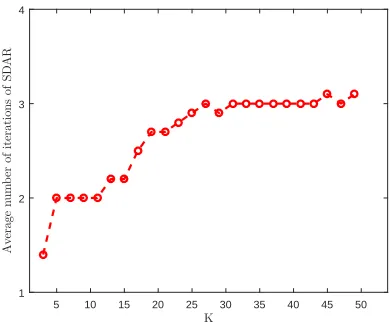
Figure 2: The average number of iterations of SDAR asK increases.
Figure 2 shows the average number of iterations of SDAR with T = K based on 100
independent replications on data sets generated from a model with (n= 500, p= 1000, K =
3 : 2 : 50, σ = 0.01, ρ = 0.1, R = 1), which will be described in Section 7.4. We can see
that as the sparsity level increases from 3 to 50 the average number of iterations of SDAR remains stable, ranging from 1 to 3, which supports the assertion in Corollary 14. More numerical comparison on number of iterations with greedy methods are shown in Section 7.2.
3.3 A brief high-level description of the proofs
The detailed proofs of Theorems 4 and 12 and their corollaries are given in the Appendix. Here we describe the main ideas behind the proofs and point out the places where the SRC and the mutual coherence condition are used.
SDAR iteratively detects the support of the solution and then solves a least squares problem on the support. Therefore, to study the convergence properties of the sequence
generated by SDAR, the key is to show that the sequence of active setsAk can approximate
A∗J more and more accurately ask increases. Let
D(Ak) =kβ¯∗|A∗
J\Akk, (35)
where k · kcan be either the `2 norm or the `∞ norm. This is a measure of the difference
betweenA∗J and Ak at the kth iteration in terms of the norm of the coefficients in A∗J but
not in Ak. A crucial step is to show that D(Ak) decays geometrically to a value bounded
by h(T) up to a constant factor, where h(T) is h2(T) defined in (12) or h∞(T) in (24).
Here h(T) is a measure of the intrinsic error due to the noise η and the approximate error
in (10). Specifically, much effort is spent on establishing the inequality (Lemma 27 in the Appendix)
D(Ak+1)≤γ∗D(Ak) +c∗h(T), k= 0,1,2, . . . , (36)
where γ∗ =γ for the `2 results in Theorem 4 and γ∗ =γµ for the `∞ results in Theorem
mutual coherence condition (A2∗) play a critical role in establishing (36). Clearly, for this
inequality to be useful, we need 0< γ∗ <1.
Another useful inequality is
kβk+1−β¯∗k ≤c1D(Ak) +c2h(T), (37)
where c1 and c2 are positive constants depending on the design matrix, see Lemma 23 in
the Appendix. The SRC and the mutual coherence condition are needed to establish this
inequality for the `2 norm and the `∞ norm, respectively. Then combining (36) and (37),
we can show part (i) of Theorem 4 and part (i) of Theorem 12.
The inequalities (36) and (37) hold for any noise vector η. Under the sub-Gaussian
assumption forη,h(T) can be controlled by the sum of unrecoverable approximation error
RJ and the universal noise levelO(σ
p
2 log(p)/n) with high probability. This leads to the
results in the remaining parts of Theorems 4 and 12, as well as Corollaries 8 and 14.
4. Adaptive SDAR
In practice, because the sparsity level of the model is usually unknown, we can use a data
driven procedure to determine an upper bound, T, for the number of important variables,
J, used in SDAR (Algorithm 1). The idea is to takeT as a tuning parameter, so T plays
a role similar to the penalty parameter λ in a penalized method. We can run SDAR
from T = 1 to a large T = L. For example, we can take L = O(n/log(n)) as suggested
by Fan and Lv (2008), which is an upper bound of the largest possible model that can
be consistently estimated with sample size n. By doing so we obtain a solution path
{βˆ(T) : T = 0,1, . . . , L}, where ˆβ(0) = 0, that is, T = 0 corresponds to the null model.
Then we use a data driven criterion, such as HBIC (Wang et al., 2013), to select a T = ˆT
and use ˆβ( ˆT) as the final estimate. The overall computational complexity of this process is
O(Lnplog(R)), see Section 5.
We can also compute the path by increasing T along a subsequence of the integers in
[1, L], for example, by taking a geometrically increasing subsequence. This will reduce the
computational cost, but here we consider the worst-case scenario.
We note that tuningT is no more difficult than tuning a continuous penalty parameter
λ in a penalized method. Indeed, we can simply increase T one by one from T = 0 to
T = L (or along a subsequence). In comparison, in tuning the value of λ based on a
pathwise solution over an interval [λmin, λmax], where λmax corresponds to the null model
and λmin > 0 is a small value, we need to determine the grid of λ values on [λmin, λmax]
as well as λmin. Here λmin corresponds to the largest model on the solution path. In the
numerical implementation of the coordinate descent algorithms for the Lasso (Friedman
et al., 2007), MCP and SCAD (Breheny and Huang, 2011), λmin =αλmaxfor a smallα, for
example,α= 0.0001. Determining the value of Lis somewhat similar to determiningλmin.
However,L has the meaning of the model size, but the meaning ofλmin is less explicit.
We also have the option to stop the iteration early according to other criterions. For
example, we can run SDAR by gradually increasing T until the change in the consecutive
solutions is smaller than a given value. Candes et al. (2006) proposed to recover β∗ based
prespecified noise levelε. Inspired by this, we can also run SDAR by increasingT gradually
until the residual sum of squares is smaller than a prespecified value ε.
We summarize these ideas in Algorithm 2 below.
Algorithm 2 Adaptive SDAR (ASDAR)
Require: Initial guess β0, d0, an integer τ, an integer L, and an early stopping criterion
(optional). Set k= 1.
1: fork= 1,2,· · · do
2: Run Algorithm 1 withT =τ kand with initial value (βk−1, dk−1). Denote the output
by (βk, dk).
3: if the early stopping criterion is satisfied orT > L then
4: stop
5: else
6: k=k+ 1.
7: end if
8: end for
Ensure: βˆ( ˆT) as estimations ofβ∗.
5. Computational complexity
We look at the number of floating point operations line by line in Algorithm 1. Clearly it
takesO(p) flops to finish step 2-4. In step 5, we use conjugate gradient (CG) method (Golub
and Van Loan, 2012) to solve the linear equation iteratively. During the CG iterations the
main operation include two matrix-vector multiplications, which cost 2n|Ak+1| flops (the
termX0yon the right-hand side can be precomputed and stored). Therefore the number of
CG iterations is smaller thanp/(2|Ak+1|), this ensures that the number of flops in step 5 is
O(np). In step 6, calculating the matrix-vector product costs np flops. In step 7, checking
the stopping condition needsO(p) flops. So the the overall cost per iteration of Algorithm 1
isO(np). By Corollary 14 it needs no more thanO(log(R)) iterations to get a good solution
for Algorithm 1 under the certain conditions. Therefore the overall cost of Algorithm 1 is
O(nplog(R)) for exactly sparse and approximately sparse case under proper conditions.
Now we consider the cost of ASDAR (Algorithm 2). Assume ASDAR is stopped when
k=L. Then the above discussion shows the the overall cost of Algorithm 2 is bounded by
O(Lnplog(R)) which is very efficient for large scale high dimension problem since the cost
increases linearly in the ambient dimensionp.
6. Comparison with greedy and screening methods
this point of view, they and SDAR share a similar characteristic. However, OMP and FoBa,
select one variable per iteration based on the current correlation, i.e., the dual variable dk
in our notation, while SDAR selectsT variables at a time based on the sum of primal (βk)
and dual (dk) information. The following interpretation in a low-dimensional setting with
a small noise term may clarify the differences between these two approaches. IfX0X/n≈I
and η≈0, we have
dk=X0(y−Xβk)/n=X0(Xβ∗+η−Xβk)/n≈β∗−βk+X0η/n≈β∗−βk,
and
βk+dk≈β∗.
Hence, SDAR can approximate the underlying supportA∗ more accurately than OMP and
Foba. This is supported by the simulation results given in Section 7.
IHT (Blumensath and Davies, 2009; Jain et al., 2014) or GraDes (Garg and Khandekar, 2009), can be formulated as
βk+1=HK(βk+skdk), (38)
whereHK(·) is the hard thresholding operator by keeping the first K largest elements and
setting others to 0. The step size sk is chosen as sk = 1 and sk = 1/(1 +δ2K) (where
δ2K is the RIP constant) for IHT and GraDes, respectively. IHT and GraDes use both
primal and dual information to detect the support of the solution, which is similar to SDAR. But when the approximate active set is given, SDAR uses least squares fitting, which is more accurate than just keeping the largest elements by hard thresholding. This is supported by the simulation results given in Section 7. Jain et al. (2014) proposed an iterative hard thresholding algorithm for general high-dimensional sparse regressions. In the linear regression setting, the algorithm proposed in Jain et al. (2014) is the same as GraDes. Jain et al. (2014) also considered a two-stage IHT, which involves a refit step on the detected support. Yuan et al. (2018) extended gradient hard thresholding for least squares loss to a general class of convex losses and analyzed the estimation and sparsity recovery performance of their proposed method. Under restricted strongly convexity (RSS) and restricted strongly smoothness conditions (RSC), Jain et al. (2014) derived an error
estimate between the approximate solutions and the oracle solution in `2 norm, which has
the same order as our result in Section 3.1. There are some differences between SDAR and
the two-stage IHT proposed in Jain et al. (2014). First, SDAR solves ann×Kleast squares
problem at each iteration while the two-stage IHT involves two least-squares problems with
larger sizes. The regularity conditions on X for SDAR concerns 2K×2K submatrices of
X, while the regularity conditions for the two-stage IHT involves larger submatries of X.
Second, our results are applicable to approximately sparse models. Jain et al. (2014) only considered exact sparse case. Third, we showed in (iii) of Corollary 3.1 that the iteration
complexity of SDAR is O(logK). In comparison, the iteration complexity of the two-stage
IHT is O(K). We also established an `∞ norm estimation result and showed that the
Fan and Lv (2008) proposed SIS for dimension reduction in ultrahigh dimensional liner
regression problems. This method selects variables with the T largest absolute values of
X0y. To improve the performance of SIS, Fan and Lv (2008) also considered an iterative
SIS, which iteratively selects more than one feature at a time until a desired number of variables are selected. They reported that the iterative SIS outperforms SIS numerically. However, the iterative SIS lacks a theoretical analysis. Interestingly, the first step in SDAR
initialized with0 is exactly the same as the SIS. But again the process of SDAR is different
from the iterative SIS in that the active set of SDAR is determined based on the sum of primal and dual approximations while the iterative SIS uses dual only.
7. Simulation Studies
7.1 Implementation
We implemented SDAR/ASDAR, FoBa, GraDes and MCP in MatLab. For FoBa, our MatLab implementation follows the R package developed by Zhang (2011a). We optimize it by keeping track of rank-one updates after each greedy step. Our implementation of MCP uses the iterative threshholding algorithm (She, 2009) with warm starts. Publicly available Matlab packages for LARS (included in the SparseLab package) are used. Since LARS and
FoBa add one variable at a time, we stop them when K variables are selected in addition
to their default stopping conditions. Of course, doing so will reduce the computation time for these algorithms as well as improve accuracy by preventing overfitting.
In GraDes, the optimal gradient step lengthskdepends on the RIP constant ofX, which
is NP hard to compute (Tillmann and Pfetsch, 2014). Here, we setsk= 1/3 following Garg
and Khandekar (2009). We stop GraDes when the residual norm is smaller than ε=√nσ,
or the maximum number of iterations is greater than n/2. We compute the MCP solution
path and select an optimal solution using the HBIC (Wang et al., 2013). We stop the
iteration when the residual norm is smaller than ε= kηk2, or the estimated support size
is greater than L =n/log(n). In ASDAR (Algorithm 2), we set τ = 50 and we stop the
iteration if the residual ky−Xβkk is smaller thanε=√nσ ork≥L=n/log(n).
7.2 Accuracy and efficiency
We compare the accuracy and efficiency of SDAR/ASDAR with Lasso (LARS), MCP, GraDes and FoBa.
We consider a moderately large scale setting withn= 5000 andp= 50000. The number
of nonzero coefficients is set to beK = 400. So the sample sizenis aboutO(Klog(p−K)).
The dimension of the model is nearly at the limit whereβ∗can be reasonably well estimated
by the Lasso (Wainwright, 2009).
To generate the design matrixX, we first generate ann×p random Gaussian matrix ¯X
whose entries are i.i.d. N(0,1) and then normalize its columns to the √n length. ThenX
is generated withX1= ¯X1, Xj = ¯Xj+ρ( ¯Xj+1+ ¯Xj−1), j = 2, . . . , p−1 andXp = ¯Xp. The
underlying regression coefficient β∗ is generated with the nonzero coefficients uniformly
distributed in [m, M], where m = σp2 log(p)/n and M = 100m. Then the observation
vector y =Xβ∗ +η with η1, . . . , ηn generated independently from N(0, σ2). We set R =
Table 1 shows the results based on 100 independent replications. The first column
gives the correlation value ρand the second column shows the methods in the comparison.
The third and the fourth columns give the averaged relative error, defined as ReErr =
Pkˆ
β−β∗k/kβ∗k, and the averaged CPU time (in seconds), The standard deviations of the
CPU times and the relative errors are shown in the parentheses. In each column of Table 1, the numbers in boldface indicate the best performers.
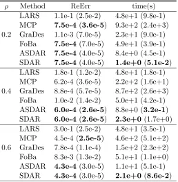
Table 1: Numerical results (relative errors, CPU times) on data sets with n = 5000, p =
50000, K = 400, R= 100, σ= 1, ρ= 0.2 : 0.2 : 0.6.
ρ Method ReErr time(s)
LARS 1.1e-1 (2.5e-2) 4.8e+1 (9.8e-1)
MCP 7.5e-4 (3.6e-5) 9.3e+2 (2.4e+3)
0.2 GraDes 1.1e-3 (7.0e-5) 2.3e+1 (9.0e-1)
FoBa 7.5e-4 (7.0e-5) 4.9e+1 (3.9e-1)
ASDAR 7.5e-4 (4.0e-5) 8.4e+0 (4.5e-1)
SDAR 7.5e-4 (4.0e-5) 1.4e+0(5.1e-2)
LARS 1.8e-1 (1.2e-2) 4.8e+1 (1.8e-1)
MCP 6.2e-4 (3.6e-5) 2.2e+2 (1.6e+1)
0.4 GraDes 8.8e-4 (5.7e-5) 8.7e+2 (2.6e+3)
FoBa 1.0e-2 (1.4e-2) 5.0e+1 (4.2e-1)
ASDAR 6.0e-4 (2.6e-5) 8.8e+0 (3.2e-1)
SDAR 6.0e-4 (2.6e-5) 2.3e+0(1.7e+0)
LARS 3.0e-1 (2.5e-2) 4.8e+1 (3.5e-1)
MCP 4.5e-4 (2.5e-5) 4.6e+2 (5.1e+2)
0.6 GraDes 7.8e-4 (1.1e-4) 1.5e+2 (2.3e+2)
FoBa 8.3e-3 (1.3e-2) 5.1e+1 (1.1e+0)
ASDAR 4.3e-4 (3.0e-5) 1.1e+1 (5.1e-1)
SDAR 4.3e-4 (3.0e-5) 2.1e+0(8.6e-2)
We see that when the correlation ρ is low, i.e., ρ = 0.2, MCP, FoBa, SDAR and
AS-DAR are on the top of the list in average error (ReErr). In terms of speed, SAS-DAR/ASAS-DAR
is about 3 to 100 times faster than the other methods. As the correlation ρ increases
to ρ = 0.4 and ρ = 0.6, FoBa becomes less accurate than SDAR/ASDAR. MCP is
similar to SDAR/ASDAR in terms of accuracy, but it is 20 to 100 times slower than SDAR/ASDAR. The standard deviations of the CPU times and the relative errors of MCP and SDAR/ASDAR are similar and smaller than those of the other methods in all the three settings.
7.3 Influence of the model parameters
In this set of simulations, the rows of the design matrix X are drawn independently
from N(0,Σ) with Σjk = ρ|j−k|,1 ≤ j, k ≤ p. The elements of the error vector η are
generated independently with ηi ∼ N(0, σ2), i = 1, . . . , n. Let R = M/m, where, M =
max{|βA∗∗|}, m= min{|βA∗∗|}= 1. The underlying regression coefficient vector β∗ ∈ Rp is
generated in such a way that A∗ is a randomly chosen subset of {1,2, ..., p} with |A∗| =
K < nandR ∈[1,103]. Then the observation vectory =Xβ∗+η. We use{n, p, K, σ, ρ, R}
to indicate the parameters used in the data generating model described above. We run
ASDAR withτ = 5, L=n/log(n) (if not specified). We use the HBIC (Wang et al., 2013)
to select the tuning parameterT. The simulation results given in Figure 3 are based on 100
independent replications.
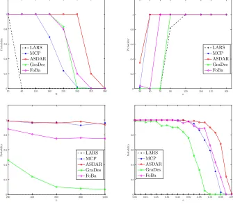
7.3.1 Influence of the sparsity level K
The top left panel of Figure 3 shows the results of the influence of sparsity level K on the
probability of exact recovery ofA∗ of ASDAR, LARS, MCP, GraDes and FoBa. Data are
generated from the model with (n= 500, p= 1000, K = 10 : 50 : 360, σ= 0.5, ρ= 0.1, R=
103).HereK = 10 : 50 : 360 means the sample size starts from 10 to 360 with an increment
of 50. We useL= 0.8nfor both ASDAR and MCP to eliminate the effect of stopping rule
since the maximum K = 360. When the sparsity level K = 10, all the solvers performed
well in recovering the true support. As K increases, LARS was the first one that failed to
recover the support and vanished when K = 60 (this phenomenon had also been observed
in Garg and Khandekar (2009), MCP began to fail whenK >110, GraDes and FoBa began
to fail whenK >160. In comparison, ASDAR was still able to do well even whenK = 260.
7.3.2 Influence of the sample size n
The top right panel of Figure 3 shows the influence of the sample sizenon the probability
of correctly estimating A∗.Data are generated from the model with (n= 30 : 20 : 200, p=
500, K= 10, σ= 0.1, ρ= 0.1, R= 10). We see that the performance of all the five methods
becomes better as n increases. However, ASDAR performs better than the others when
n= 30 and 50. These simulation results indicate that ASDAR is more capable of handling
high-dimensional data whenp/n is large in the generating models considered here
7.3.3 Influence of the ambient dimension p
The bottom left panel of Figure 3 shows the influence of ambient dimension p on the
performance of ASDAR, LARS, MCP, GraDes and FoBa. Data are generated from the
model with (n= 100, p= 200 : 200 : 1000, K = 20, σ = 1, ρ= 0.3, R= 10). We see that
the probabilities of exactly recovering the support of the underlying coefficients of ASDAR
and MCP are higher than those of the other solvers as p increasing, which indicate that
ASDAR and MCP are more robust to the ambient dimension.
7.3.4 Influence of correlation ρ
The bottom right panel of Figure 3 shows the influence of correlationρ on the performance
of ASDAR, LARS, MCP, GraDes and FoBa. Data are generated from the model with
all the solvers becomes worse when the correlationρincreases. However, ASDAR generally
performed better than the other methods asρ increases.
10 60 110 160 210 260 310 360
K 0 0.2 0.4 0.6 0.8 1 P ro b a b il it y LARS MCP ASDAR GraDes FoBa
30 50 70 90 120 150 170 200
n 0 0.2 0.4 0.6 0.8 1 P ro b a b il it y LARS MCP ASDAR GraDes FoBa
200 400 600 800 1000
p 0 0.2 0.4 0.6 0.8 1 P ro b a b il it y LARS MCP ASDAR GraDes FoBa
0.05 0.15 0.25 0.35 0.45 0.55 0.65 0.75 0.85 0.95
ρ 0 0.2 0.4 0.6 0.8 1 P ro b a b il it y LARS MCP ASDAR GraDes FoBa
Figure 3: Numerical results of the influence of sparsity levelK (top left panel), sample size
n (top right panel), ambient dimension p (bottom left panel) and correlation ρ
(bottom right panel) on the probability of exact recovery of the true support of all the solvers considered here.
In summary, our simulation studies demonstrate that SDAR/ASDAR is generally more accurate, more efficient and more stable than Lasso, MCP, FoBa and GraDes.
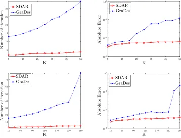
7.4 Number of iterations
In this subsection we compare SDAR with GraDes (IHT) in terms of the number of iter-ations. We run 100 independent replications on data sets generated from the models with
(n = 500, p= 1000, K = 5 : 5 : 55, σ = 0.05, ρ= 0, R = 1) and (n= 2000, p= 5000, K =
10 : 20 : 250, σ = 0.05, ρ = 0, R = 1) described in Section 7.3. The average number of
iteration (left column) and average absolute error in `∞ norm (right column) are displayed
in Figure 4. We can see that the number of iterations of GraDes increases almost
sub-linearly as the sparsity level K increases while that of SDAR almost varies little. And in
5 15 25 35 45 55 5
10 15 20 25 30
5 15 25 35 45 55
10-3
10-2
10-1
100
10 50 90 130 170 210 250
10 20 30 40 50 60 70
10 50 90 130 170 210 250
10-3
10-2
10-1
100
Figure 4: Comparisons the dependence of number of iterations (left panels) and accuracy
(right panels) on sparsity levelK with data set (n= 500, p= 1000, K = 5 : 5 :
55, σ = 0.05, ρ = 0.3, R = 1) and (n = 2000, p = 5000, K = 10 : 20 : 250, σ =
0.05, ρ= 0.3, R= 1).
8. Concluding remarks
SDAR is a constructive approach for fitting sparse, high-dimensional linear regression
mod-els. Under appropriate conditions, we established the nonasymptotic minimax `2 error
bound and optimal `∞ error bound of the solution sequence generated by SDAR. We also
calculated the number of iterations required to achieve these bounds. In particular, an interesting and surprising aspect of our results is that, under a mutual coherence condition on the design matrix, the number of iterations required for the SDAR to achieve the
op-timal `∞ bound does not depend on the underlying sparsity level. In addition, SDAR has
the same computational complexity per iteration as LARS, coordinate descent and greedy methods. Our simulation studies demonstrate that SDAR/ASDAR is accurate, fast, stable and easy to implement, and it is competitive with or outperforms the Lasso, MCP and two greedy methods in efficiency and accuracy in the generating models we considered. These theoretical and numerical results suggest that SDAR/ASDAR is a useful addition to the literature on sparse modeling.
It would also be interesting to develop parallel or distributed versions of SDAR that can
run on multiple cores for data sets with bignand largepor for data that are distributively
stored.
We have implemented SDAR in a Matlab package sdar, which is available at http:
//homepage.stat.uiowa.edu/~jian/.
Acknowledgments
We are grateful to the action editor and the anonymous reviewers for their detailed and constructive comments which led to considerable improvements in the paper. We also thank Patrick Breheny for his critical reading of the paper and providing helpful comments. This research is supported in part by the National Science Foundation of China (NSFC) grants 11501579, 11571263, 11471253, 91630313, 11871385, 11871474 and 11801531.
Appendix A
Proof of Lemma 1.
Proof Let Lλ(β) = 21nkXβ−yk22+λkβk0. Supposeβ is a coordinate-wise minimizer of
Lλ. Then
βi ∈argmin
t∈R
Lλ(β1, ..., βi−1, t, βi+1, ..., βp)
⇒ βi ∈argmin
t∈R 1 2nkXβ
−
y+ (t−βi)Xik22+λ|t|0
⇒ βi ∈argmin
t∈R 1 2(t−β
i)2+n1(t−β
i)X
0
i(Xβ
−
y) +λ|t|0
⇒ βi ∈argmin
t∈R 1 2(t−(β
i +X
0
i(y−Xβ
)/n))2+λ|t|0.
Letd=X0(y−Xβ)/n. By the definition of the hard thresholding operatorHλ(·) in (5),
we have
βi =Hλ(βi+di) fori= 1, ..., p,
which shows (4) holds.
Conversely, suppose (4) holds. Let
A= n
i∈S|βi+di| ≥
√
2λ
o
.
By (4) and the definition ofHλ(·) in (5), we deduce that for i∈A, |βi| ≥
√
2λ.
Further-more,0=dA =XA0(y−XAβ
A)/n,which is equivalent to
βA ∈argmin21nkXAβA−yk2
2. (39)
Next we show Lλ(β +h) ≥Lλ(β) if h is small enough with khk∞ <
√
2λ. We consider
two cases. If h(A)c 6= 0, then
Lλ(β+h)−Lλ(β)≥ 21nkXβ−y+Xhk22− 21nkXβ
−yk2
which is positive for sufficiently small h. If h(A)c = 0, by the minimizing property of βA
in (39) we deduce that Lλ(β+h)≥Lλ(β). This completes the proof of Lemma 1.
Lemma 20 Let A and B be disjoint subsets of S, with |A| = a and |B| = b. Assume
X ∼SRC(a+b, c−(a+b), c+(a+b)). Let θa,b be the sparse orthogonality constant and let
µ be the mutual coherence of X. Then we have
nc−(a)≤
XATXA
≤nc+(a), (40)
1
nc+(a) ≤
(XATXA)−1
≤
1
nc−(a)
, (41)
XA0
≤
p
nc+(a) (42)
θa,b≤(c+(a+b)−1)∨(1−c−(a+b)) (43) kXB0 XAuk∞≤naµkuk∞, ∀u∈R|A|, (44)
kXAk= XA0
≤
p
n(1 + (a−1)µ). (45)
Furthermore, ifµ <1/(a−1), then
k(XA0 XA)−1uk∞≤
kuk∞
n(1−(a−1)µ), ∀u∈R
|A|
. (46)
Moreover, c+(s) is an increasing function of s,c−(s) a decreasing function ofsand θa,ban
increasing function of aand b.
Proof The assumption X ∼ SRC(a, c−(a), c+(a)) implies the spectrum of XA0 XA/n is
contained in [c−(a), c+(a)]. So (40) - (42) hold. Let I be an (a+b)×(a+b) identity
matrix. (43) follows from the fact thatXA0 XB/nis a submatrix ofXA0 ∪BXA∪B/n−Iwhose
spectrum norm is less than (1−c−(a+b))∨(c+(a+b)−1). Let G = X0X/n. Then,
|Paj=1Gi,juj| ≤µakuk∞,for alli∈B, which implies (44). By Gerschgorin’s disk theorem,
| kGA,Ak −Gi,i| ≤ a X
i6=j=1
|Gi,j| ≤(a−1)µ ∀i∈A,
thus (45) holds. For (46), it suffices to showkGA,Auk∞≥(1−(a−1)µ)kuk∞ifµ <1/(a−1).
In fact, let i∈Asuch that kuk∞=|ui|, then
kGA,Auk∞≥ |
a X
j=1
Gi,juj| ≥ |ui| − a X
i6=j=1
|Gi,j| |uj| ≥ kuk∞−µ(a−1)kuk∞.
The last assertion follows from their definitions. This completes the proof of Lemma 20.
Lemma 21 Suppose (A3) holds. We have for anyα∈(0,1/2),
PkX0ηk∞≤σp2 log(p/α)n≥1−2α, (47)
P
max
|A|≤T
kXA0 ηk2≤σ
√
Tp2 log(p/α)n
Proof This lemma follows from the sub-Gaussian assumption (A3) and standard proba-bility calculation, see Zhang and Huang (2008); Wainwright (2009) for details.
We now define some notation that will be useful in proving Theorems 4 and 12. For
any given integers T and J with T ≥J and F ⊆S with|F|=T−J, let A◦ =A∗J∪F and
I◦ = (A◦)c. Let{Ak}
k be the sequence of active sets generated by SDAR (Algorithm 1).
Define
D2(Ak) =kβ¯∗|A∗
J\Akk2 and D∞(A
k) =kβ¯∗|
A∗\Akk ∞.
These quantities measure the differences between Ak and A∗J in terms of the `2 and `∞
norms of the coefficients inA∗J but not in Ak. A crucial step in our proofs is to control the
sizes of these measures. Let
Ak1 =Ak∩A◦, Ak2 =A◦\Ak1, I3k =Ak∩I◦, I4k =I◦\I3k.
Denote the cardinality of I3k by lk=|I3k|. Let
Ak11=Ak1\(Ak+1∩Ak1), Ak22=Ak2\(Ak+1∩Ak2), I33k =Ak+1∩I3k, I44k =Ak+1∩I4k,
and
4k=βk+1−β¯∗|Ak.
These notation can be easily understood in the case T = J. For example, D2(Ak) and
D∞(Ak) are measures of the difference between the active set Ak and the target support
A∗J. Ak
1 andI3k contain the correct indices and incorrect indices inAk, respectively. Ak11and
Ak22include the indices inA◦that will be lost from thekth iteration to the (k+1)th iteration.
I33k and I44k contain the indices included in I◦ that will be gained from the kth iteration
to the (k+ 1)th iteration. By Algorithm 1, we have |Ak| = |Ak+1| = T, Ak = Ak
1 ∪I3k, |Ak2|=|A◦| − |Ak1|=|A◦| − |I3k|=T−(T−lk) =lk ≤T, and
|Ak11|+|Ak22|=|I33k|+|I44k |, (49)
D2(Ak) =kβ¯∗|A◦\Akk 2 =kβ¯
∗|
Ak
2k2, (50)
D∞(Ak) =kβ¯∗|A◦\Akk
∞=kβ¯ ∗|
Ak
2k∞. (51)
In Subsection 3.3, we described the overall approach for proving Theorems 4 and 12. Before proceeding to the proofs, we break down the argument into the following steps.
1. In Lemma 22 we show that the effects of the noise and the approximation model
(10) measured by h2(T) and h∞(T) can be controlled by the sum of unrecoverable
approximation error RJ and the universal noise level O(σ
p
2 log(p)/n) with high
probability, provided that η is sub-Gaussian.
2. In Lemma 23 we show that the`2norms (`∞norms) of4kandβk−β¯∗ are controlled
in terms ofD2(Ak) and h2(T) (D∞(Ak) and h∞(T)).
3. In Lemma 24 we show that D2(Ak+1) (D∞(Ak+1)) can be bounded by the norm of
¯
β∗ on the lost indices, which in turn can be controlled in terms ofD2(Ak) and h2(T)
4. In Lemma 25 we make use of the orthogonality between βk and dk to show that the
norms ofβk+1anddk+1on the lost indices can be bounded by the norm on the gained
indices. Lemma 26 gives the upper bound of the norms ofβk+1anddk+1on the gained
indices by the sum of D2(Ak),h2(T) (D∞(Ak), h∞(T)), and the norm of4k.
5. We combine Lemmas 22-26 and get the desired relations between D2(Ak+1) and
D2(Ak) (D∞(Ak+1) andD∞(Ak)) in Lemma 27.
Then we prove Theorems 4 and 12 based on Lemma 27, (56) and (58).
Lemma 22 Let A⊂S with |A| ≤T. Suppose (A1) and (A3) holds. Then for α∈(0,1/2)
with probability at least 1−2α, we have
(i) If X∼SRC(T, c−(T), c+(T)), then
h2(T)≤ε1, (52)
where ε1 is defined in (18). (ii) We have
h∞(T)≤ε2, (53)
where ε2 is defined in (29). Proof We first show
kXβ∗|(A∗
J)ck2 ≤
p
nc+(J)RJ, (54)
under the assumption ofX ∼SRC(c−(T), c+(T), T) and (A1). In fact, letβbe an arbitrary
vector inRp andA1 be the firstJ largest positions ofβ,A2 be the next and so forth. Then
kXβk2 ≤ kXβA1k2+
X
i≥2
kXβAik2 ≤pnc+(J)kβA1k2+
p
nc+(J)
X
i≥2
kβAik2
≤pnc+(J)kβk2+
p
nc+(J)
X
i≥1
r 1
JkβAi−1k1
≤pnc+(J)(kβk2+
r 1
Jkβk1),
where the first inequality follows from the triangle inequality, the second inequality follows from (42), and the third and fourth ones follows from simple algebra. This implies (54)
holds by observing the definition of RJ. By the triangle inequality, (42), (54) and (48), we
have with probability at least 1−2α,
kXA0 η¯k2/n≤ kXA0 Xβ∗|(A∗
J)ck2/n+kX 0
Aηk2/n ≤c+(J)RJ+σ
√
Therefore, (52) follows by noticing the monotone increasing property ofc+(·), the definition
of ε1 in (18) and the arbitrariness ofA.
By a similar argument for (54) and replacing pnc+(J) with
p
n(1 + (J−1)µ) based
on (45), we get
kXβ∗|(A∗
J)ck2 ≤
p
n(1 + (K−1)µ)RJ. (55)
Therefore, by (45), (55) and (47), we have with probability at least 1−2α,
kXA0 η¯k∞/n≤ kXA0 Xβ∗|(A∗
J)ck∞/n+kX 0
Aηk2/n ≤ kXA0 Xβ∗|(A∗
J)ck2/n+kX 0
Aηk2/n
≤(1 + (J−1)µ)RJ+σ
p
2 log(p/α)/n.
This implies part (ii) of Lemma 22 by noticing the definition ofε2 in (29) and the
arbitrari-ness ofA. This completes the proof of Lemma 22.
Lemma 23 Let A⊂S with|A| ≤T. Suppose (A1) holds.
(i) If X∼SRC(T, c−(T), c+(T)),
kβk+1−β¯∗k2 ≤1 + θT ,T
c−(T)
D2(Ak) +
h2(T)
c−(T)
, (56)
and
k4kk2 ≤ θT,T
c−(T) kβ¯∗|Ak
2k2+
h2(T)
c−(T)
. (57)
(ii) If (T −1)µ <1, then
kβk+1−β¯∗k∞≤ 1 +µ
1−(T−1)µD∞(A
k) + h∞(T)
1−(T−1)µ, (58)
and
k4kk∞≤ T µ
1−(T −1)µkβ¯
∗|
Ak
2k∞+
h∞(T)
(1−(T−1)µ). (59)
Proof We have
βAk+1k = (X 0
AkXAk)−1XA0ky
= (XA0kXAk)−1XA0k(XAk
1 ¯
βA∗k
1 +XA
k
2 ¯
βA∗k
2 + ¯η), (60)
( ¯β∗|Ak)Ak = (XA0kXAk)−1XA0kXAk( ¯β∗|Ak)Ak
= (XA0kXAk)−1XA0k(XAk
1 ¯
βA∗k
where the first equality uses the definition of βk+1 in Algorithm 1, the second equality
follows from y = Xβ¯∗+ ¯η =XAk
1 ¯
βA∗k
1
+XAk
2 ¯
βA∗k
2
+ ¯η, the third equality is simple algebra,
and the last one uses the definition ofAk1.Therefore,
k4kk2=kβAk+1k −( ¯β ∗|
Ak)Akk 2
=k(XA0kXAk)−1XA0k(XAk
2 ¯
βA∗k
2 + ¯η)
k 2 ≤ 1
nc−(T)
(kXA0kXAk
2 ¯
βA∗k
2
k 2+kX
0
Akη¯k2) ≤ θT ,T
c−(T) kβ¯∗|Ak
2k2+
h2(T)
c−(T)
,
where the first equality uses supp(βk+1) =Ak, the second equality follows from (61) and
(60), the first inequality follows from (41) and the triangle inequality, and the second
in-equality follows from (50), the definition of θa,b and the definition of h2(T). This proves
(57). Then the triangle inequalitykβk+1−β¯∗k2≤ kβk+1−β¯∗|Akk2+kβ¯∗|A◦\Akk
2 and (57)
imply (56).
Using an argument similar to the proof of (57) and by (46), (44) and (51), we can show (59). Thus (58) follows from the triangle inequality and (59). This completes the proof of Lemma 23.
Lemma 24
D2(Ak+1)≤ kβ¯A∗k
11
k 2+k
¯
β∗Ak
22
k
2, (62)
D∞(Ak+1)≤ kβ¯A∗k
11
k ∞+k
¯
βA∗k
22
k
∞. (63)
kβ¯A∗k
11
k
2≤ k4
k Ak
11
k 2+kβ
k+1
Ak
11
k
2, (64)
kβ¯A∗k
11
k
∞≤ k4
k Ak
11
k
∞+kβ
k+1
Ak
11
k
∞. (65)
Furthermore, assume (A1) holds. We have
kβ¯A∗k
22
k
∞≤ kd
k+1
Ak
22
k
∞+T µk4
k
Akk∞+T µD∞(Ak) +h∞(T), (66)
kβ¯A∗k
22
k 2 ≤
kdk+1
Ak
22
k
2+θT ,Tk4
k
Akk2+θT,TD2(Ak) +h2(T)
c−(T)
if X ∼SRC(T, c−(T), c+(T)).
(67)
Proof By the definitions of D2(Ak+1), Ak11,Ak11 andAk22, we have
D2(Ak+1) =kβ¯∗|A◦\Ak+1k
2=kβ¯ ∗|
Ak
11∪Ak22k2 ≤ k
¯
βA∗k
11
k 2+k
¯
βA∗k
22
k 2.
This proves (62). (63) can be proved similarly. To show (64), we note that 4k =βk+1−
¯
β∗|Ak. Thus
kβkA+1k
11
k 2=
kβ¯∗ Ak
Ak
11
+4kAk
11
k 2
≥ kβ¯A∗k
11
k 2− k4
k Ak
11