Aligning Domain-Specific Distribution and Classifier for Cross-Domain Classification from Multiple Sources

The Thirty-Third AAAI Conference on Artificial Intelligence (AAAI-19)

Aligning Domain-Specific Distribution and Classifier

for Cross-Domain Classification from Multiple Sources

Yongchun Zhu,

Fuzhen Zhuang,

Deqing Wang

1_{Key Lab of Intelligent Information Processing of Chinese Academy of Sciences (CAS),}

Institute of Computing Technology, CAS, Beijing 100190, China

2_{University of Chinese Academy of Sciences, Beijing 100049, China} 3_{School of Computer Science, Beihang University, Beijing, China}

{zhuyongchun18s, zhuangfuzhen}@ict.ac.cn, [email protected]

Abstract

While Unsupervised Domain Adaptation (UDA) algorithms, i.e., there are only labeled data from source domains, have been actively studied in recent years, most algorithms and theoretical results focus on Single-source Unsupervised Do-main Adaptation (SUDA). However, in the practical scenario, labeled data can be typically collected from multiple diverse sources, and they might be different not only from the target domain but also from each other. Thus, domain adapters from multiple sources should not be modeled in the same way. Re-cent deep learning based Multi-source Unsupervised Domain Adaptation (MUDA) algorithms focus on extracting common domain-invariant representations for all domains by aligning distribution of all pairs of source and target domains in a com-mon feature space. However, it is often very hard to extract the same domain-invariant representations for all domains in MUDA. In addition, these methods match distributions with-out considering domain-specific decision boundaries between classes. To solve these problems, we propose a new frame-work with two alignment stages for MUDA which not only respectively aligns the distributions of each pair of source and target domains in multiple specific feature spaces, but also aligns the outputs of classifiers by utilizing the domain-specific decision boundaries. Extensive experiments demon-strate that our method can achieve remarkable results on pop-ular benchmark datasets for image classification.

Introduction

Recent advances in deep learning have significantly im-proved the state-of-the-arts across a variety of visual learn-ing tasks (Ren et al. 2015; He et al. 2016). These achieve-ments mainly come from the availability of large-scale la-beled data for supervised learning. For a target task with the shortage of labeled data, there is a strong motivation to build effective learners that can leverage rich labeled data from a related source domain. However, due to the presence of domain shift (Quionero-Candela et al. 2009; Pan and Yang 2010), the performance of the learned model might tend to degrade heavily in the target domain.

Learning a discriminative model in the presence of do-main shift between training and test distributions is known

∗

Corresponding author: Fuzhen Zhuang

Copyright c2019, Association for the Advancement of Artificial Intelligence (www.aaai.org). All rights reserved.

Single-source domain

adaptation

Multi-source domain

adaptation

target source1 source2 source3

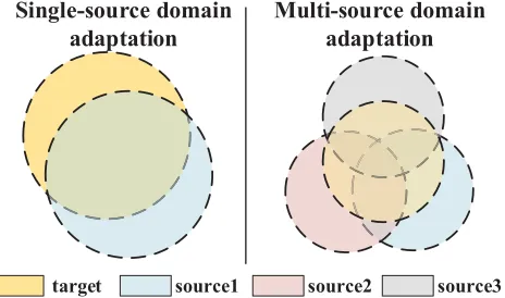
Figure 1: In Single-source Unsupervised Domain Adapta-tion (SUDA), the distribuAdapta-tion of source and target domains cannot be matched very well. While in Multi-source Unsu-pervised Domain Adaptation (MUDA), due to the shift be-tween multiple source domains, it is much harder to match distributions of all source domains and target domains. (Best viewed in color.)

as domain adaptation. In recent years, most domain adap-tation algorithms focus on Single-source Unsupervised Do-main Adaptation (SUDA) problem, where there are only la-beled data from one single source domain. Previous SUDA methods include re-weighting the training data (Jiang and Zhai 2007; Huang et al. 2007), and finding a transforma-tion in a lower-dimensional manifold that draws the source and target subspaces closer (Gong et al. 2012; Fernando et al. 2013). In recent years, most SUDA algorithms learn to map the data from both domains into a common fea-ture space to learn domain-invariant representations by min-imizing domain distribution discrepancy (Long et al. 2015; Ganin and Lempitsky 2015; Sun and Saenko 2016; Long et al. 2017), and the source classifier can then be directly ap-plied to target instances.

Tsang 2012; Jhuo et al. 2012; Liu, Shao, and Fu 2016). It is a common and straightforward way to combine all source domains into one single source domain and align distribu-tions as SUDA methods do. Due to the data expansion, the methods might improve the performance. However, the im-provement might not be significant, hence, it is necessary to find a better way to make full use of multiple source do-mains.

Despite the rapid progress in deep learning based SUDA, a few studies have been given to deep learning based MUDA, which is much more challenging (Xu et al. 2018). In recent years, some works on deep learning for MUDA are proposed, and there are two common problems exist in these methods. First, they try to map all source and target domain data into a common feature space to learn common domain-invariant representations. However, it is not easy to learn domain-invariant representations even for one single source and one target domain data. As an intuitive example in Figure 1, we can not remove the shift between one sin-gle source and one target domains, and when we try to align multiple source and target domains, the bigger mismatch de-gree might lead to unsatisfying performance. Second, they assume that the target domain data can be classified cor-rectly by multiple domain-specific classifiers because they are aligned with the source domain data. However, these methods might fail to extract discriminative features because it does not consider the relationship between target samples and the domain-specific decision boundary when aligning distributions.

In this paper, we propose a new framework with two-stage alignments for MUDA to overcome both problems. The first stage is aligning the domain-specific distribution, i.e., we respectively map each pair of source and target domains data into multiple different feature spaces, and align domain-specific distributions to learn multiple domain-invariant rep-resentations. Then we train multiple domain-specific classi-fiers using multiple domains-invariant representations. The second stage is aligning domain-specific classifiers. The tar-get samples near domain-specific decision boundary pre-dicted by different classifiers might get the different labels. Hence, utilizing the domain-specific decision boundaries, we align the classifiers’ output for the target samples. Ex-tensive experiments show that our method can obtain re-markable results for MUDA on public benchmark datasets compared to the state-of-the-art methods.

The contributions of this paper are summarized as fol-lows. (1) We propose a new two-stage alignment framework for MUDA which aligns the domain-specific distributions of each pair of source and target domains in multiple feature spaces and align the domain-specific classifiers’ output for target samples. (2) We conduct comprehensive experiments on three well-known benchmarks, and the experimental re-sults validate the effectiveness of the proposed model.

Related Work

In this section, we will introduce the related work in two aspects: Single-source Unsupervised Domain Adaptation (SUDA) and Multi-source Unsupervised Domain Adapta-tion (MUDA).

Single-source Unsupervised Domain Adaptation (SUDA). Recent years have witnessed many ap-proaches to solve the visual domain adaptation prob-lem, which is also commonly framed as the visual dataset bias problem (Quionero-Candela et al. 2009; Pan and Yang 2010). Previous shallow meth-ods for SUDA include re-weighting the train-ing data so that they could more closely reflect those in the test distribution (Jiang and Zhai 2007; Huang et al. 2007), and finding a transformation in a lower-dimensional manifold that draws the source and target subspaces closer (Gong et al. 2012; Pan et al. 2011; Fernando et al. 2013).

Some recent works bridge deep learning and domain adaptation (Long et al. 2015; Ganin and Lempitsky 2015; Tzeng et al. 2017; Sun and Saenko 2016). The two main-streams: the one extends deep convolutional networks to do-main adaptation by adding adaptation layers through which the mean embeddings of distributions are matched (Tzeng et al. 2014; Long et al. 2015; 2017), while the other by adding a subnetwork as domain discriminator and the deep fea-tures are learned to confuse the discriminator in a domain-adversarial training paradigm (Ganin and Lempitsky 2015; Tzeng et al. 2017; Saito et al. 2017). And recent related work extends the adversarial methods to a generative adversarial way (Bousmalis et al. 2017; Hoffman et al. 2018).

Besides of these two mainstreams, there are diverse meth-ods to learn domain-invariant features: DRCN (Ghifary et al. 2016) reconstructs features to images and makes the transformed images are similar to original images. D-CORAL (Sun and Saenko 2016) “recolors” whitened source features with the covariance of features from the target do-main.

Multi-source Unsupervised Domain Adaptation (MUDA). The SUDA methods mentioned above mainly consider one single source and one target domain. However, in practice, there are multiple source domains available. Due to the dataset shift among them, we can not use SUDA methods by combining all source domains into one single source domain. The research originates from A-SVM (Yang, Yan, and Hauptmann 2007) that lever-ages the ensemble of source-specific classifiers to tune the target categorization model, and there have been a variety of shallow models invented to tackle the MUDA problem (Duan, Xu, and Tsang 2012; Jhuo et al. 2012; Liu, Shao, and Fu 2016). MUDA also develops with theo-retical supports (Ben-David et al. 2010; Blitzer et al. 2008; Liu, Shao, and Fu 2016). Blitzer et al. (Blitzer et al. 2008) provided the first learning bound for MUDA. Mansour et al. (Mansour, Mohri, and Rostamizadeh 2009) claimed that an ideal target hypothesis can be represented by a distribution weighted combination of source hypotheses. However, in our method, we just use the average of source hypotheses as the target hypothesis.

accord-ing to the confusion loss. Zhao et al. (Zhao et al. 2018) pro-posed to combine the gradient of multiple domain discrim-inators. These work focus on extracting common domain-invariant representations for all domains. However, as men-tioned above, it is hard to learn common domain-invariant representations for all domains. Hence, we try to respec-tively map each pair of source and target domain into multi-ple feature spaces and extract multimulti-ple domain-invariant rep-resentations. In addition, utilizing the domain-specific deci-sion boundaries, we align the classifiers’ output for the target samples.

Method

In multi-source unsupervised domain adaptation, there are N different underlying source distributions denoted as {psj(x, y)}Nj=1, and the labeled source domain data

{(Xsj, Ysj)}Nj=1are drawn from these distributions

respec-tively, where Xsj = {xsj_i }|Xsj|

i=1 represents samples from

source domainj andYsj = {y sj i }

|Xsj|

i=1 is the

correspond-ing ground-truth labels. Also, we have target distribution

pt(x, y), from which target domain dataXt ={xt i}

|Xt| i=1 are

sampled yet without label observationYt.

In recent years, some works bridge deep learning and multi-source domain adaptation (Xu et al. 2018; Zhao et al. 2018), and they minimize a distance loss between each pair of source and target domains to learn common domain-invariant representations in a common feature space for all domains. The formal representation can be:

min

F,C N

X

j=1

Ex∼XsjJ(C(F(x sj i )),y

sj i )

+λ

N

X

j=1

ˆ

D(F(Xsj), F(Xt)),

(1)

whereJ(·,·) is the cross-entropy loss function (classifica-tion loss) andDˆ(·,·)is an estimate of the discrepancy be-tween two domains, such as MMD (Gretton et al. 2012; Long et al. 2015), CORAL (Sun and Saenko 2016), Con-fusion loss (Ganin and Lempitsky 2015; Tzeng et al. 2015).

F(·)is the feature extractor to map all domains into a com-mon feature space, and C(·) is the classifier. The com-mon problem with these methods is that they mainly fo-cus on learning common domain-invariant representations for all domains and do not consider domain-specific deci-sion boundaries between classes. However, it is not an easy task. Actually, extracting domain-invariant representations for each pair of source and target domains respectively is easier than extracting common domain-invariant representa-tions for all domains. In addition, the target samples near domain-specific decision boundary predicted by different classifiers might get the different labels. Hence, utilizing the domain-specific decision boundaries, we align the clas-sifiers’ outputs for the target samples. Therefore, we propose a new two-stage alignment framework to overcome these problems.

First alignment stage is aligning the domain-specific dis-tributions for each pair of source and target domains. The way to extract multiple domain-invariant representations for each pair of source and target domain is that mapping each of them into specific feature spaces and matching their distri-butions. To map each pair of source and target domains into a specific feature space, the easiest way is to train multiple networks. However, this would spend a lot of time. Hence, we propose to divide the network into two part. Specifically, the first part shares a subnetwork to learn some common features for all domains, and the second part contains N

domain-specific subnetworks that do not share the weights with each other for each pair of source and target domains. For each unshared subnetwork, we learn a domain-specific classifier. However, the target samples near domain-specific decision boundary predicted by different classifiers might get the different labels. Hence, utilizing the domain-specific decision boundaries, the second alignment stage is aligning the domain-specific classifiers’ output for the target samples. In paper (Xu et al. 2018), they proposed a complex voting method for multiple classifiers, in our method the complex voting method is not needed due to the second stage align-ment.

Two-stage alignment Framework

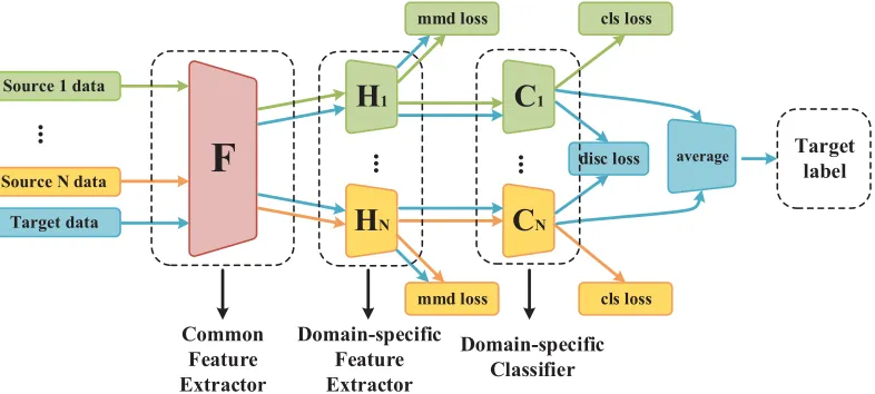
Our framework consists of three components, i.e., a com-mon feature extractor, domain-specific feature extractors, domain-specific classifiers, as shown in Figure 2.

Common feature extractorWe propose a common sub-networkf(·)to extract common representations for all do-mains, which map the images from the original feature space into a common feature space.

Domain-specific feature extractor We want each pair of source and target domain data could be mapped into a specific feature space. Given a batch images xsj from source domain (Xsj, Ysj) and a batch images xt _from

target domain Xt, these domain-specific feature extrac-tors receive the common features f(xsj_{) andf(x}t_{) from}

common feature extractor. Then, there are N unshared domain-specific subnetworkshj(·)for each source domain

(Xsj, Ysj), which map each pair of source and target

do-mains into a specific feature space.

The aim of deep domain adaptation is to learn domain-invariant representations, and there are several methods to achieve this goal in recent years, such as mmd loss (Gret-ton et al. 2012; Long et al. 2015), adversarial loss (Ganin and Lempitsky 2015; Tzeng et al. 2015), coral loss (Sun and Saenko 2016), reconstruction loss (Ghifary et al. 2016). Here we choose the MMD method to reduce the distribution discrepancy between domains.

Domain-specific classifierC is a multi-output net com-posed byN domain-specific predictor{Cj}N

j=1. Each

pre-dictor Cj is a softmax classifier, and receives the specific

Source 1 data

Source N data

Target data

F

C

C

mmd loss

cls loss

cls loss disc loss

...

H

H

Target label

...

...

Common Feature Extractor

Domain-specific Feature Extractor

Domain-specific Classifier

Figure 2: An overview of the proposed two-stage alignment framework. Our framework receives multi-source instances with annotated ground truth and adapts to classifying the target samples. There are specific feature extractors and classifiers for each source. (Best viewed in color.)

formulated as:

Lcls= N

X

j=1

Ex∼XsjJ(Cj(Hj(F(x sj i ))),y

sj

i ). (2)

Domain-specific Distribution Alignment

To achieve the first alignment stage (align distributions for each pair of source and target domains), we choose Maxi-mum Mean Discrepancy (MMD) (Gretton et al. 2012) as our estimate of the discrepancy between two domains. MMD is a kernel two-sample test which rejects or accepts the null hypothesisp = qbased on the observed samples. The ba-sic idea behind MMD is that if the generating distributions are identical, all the statistics are the same. Formally, MMD defines the following difference measure:

DH(p, q),kEp[φ(xs)]−Eq[φ(xt)]k2H, (3) whereHis the reproducing kernel Hillbert space (RKHS) endowed with a characteristic kernelk. Hereφ(·)denotes some feature map to map the original samples to RKHS and the kernelkmeansk(xs_,xt_{) =hφ(x}s_{), φ(x}t_{)iwhereh·,·i}

represents inner product of vectors. The main theoretical re-sult is thatp= q if and only ifDH(p, q) = 0(Gretton et al. 2012). In practice, an estimate of the MMD compares the square distance between the empirical kernel mean embed-dings as

ˆ

DH(p, q) =

1

ns

X

xi∈Ds

φ(xi)−

1

nt

X

xj∈Dt φ(xj)

2

H

, (4)

whereDˆH(p, q)is an unbiased estimator ofDH(p, q). We use Equation (4) as the estimate of the discrepancy between each source domain and target domain. The MMD loss is reformulated as:

Lmmd=

1

N N

X

j=1

ˆ

D(Hj(F(Xsj)), Hj(F(Xt))), (5)

Each specific feature extractor could learn domain-invariant representations for each pair of source and target domain by minimizing the Equation 5.

Domain-specific Classifier Alignment

The target samples near the class boundaries are more likely to be misclassified by the classifiers learned from source samples. The classifiers are trained on different source do-mains, hence they might have the disagreement on the pre-diction for target samples especially the target samples near class boundaries. Intuitively, the same target sample pre-dicted by different classifiers should get the same prediction. Hence, the second alignment stage is to minimize the dis-crepancy among all classifiers. In this paper, we utilize the absolute values of the difference between all pairs of classi-fiers’ probabilistic outputs of target domain data as discrep-ancy loss:

Ldisc=

2

N×(N−1)

N−1 X

j=1 N

X

i=j+1

Ex∼Xt[|Ci(Hi(F(xk)))

−Cj(Hj(F(xk)))|],

(6)

In (Xu et al. 2018), they propose a target classification oper-ator to combine the multiple source classifiers. However, it is complex to vote the label for target samples. By minimizing the Equation (6), the probabilistic outputs of all classifiers are similar. Finally, to predict the labels of target samples, we compute the average of all classifier outputs.

Algorithm 1Multiple Feature Spaces Adaptation Network (MFSAN)

1: Give the number of training iterationsT 2: fortin 1 :T do

3: Randomly samplemimages{xsj_i , ysj_i }m

i=1from one

ofNsource domains{(Xsj, Ysj)}N j=1. 4: Samplemimages{xt

i}mi=1from target domain(Xt). 5: Feed source and target samples to common feature extractor to get the common latent representations

F(xsj_i )andF(xt i).

6: Feed common latent representations of source sam-ples to domain-specific feature extractor to get domain-specific representations of source samples

Hj(F(x sj i )).

7: Feed domain-specific representations of source sam-plesHj(F(x

sj

i ))to domain-specific classifier to get Cj(Hj(F(x

sj

i ))), and the classification is computed

as Equation (2).

8: Feed common latent representation of target samples to all domain-specific extractor to get domain-specific representations of target samples

H1(F(xit1)),· · ·, HN(F(x tN i )), 9: Use Hj(F(xsj_i ))andHj(F(xt1

i ))to calculate mmd

loss as Equation (5).

10: Use H1(F(xti1)),· · · , HN(F(xtNi ))to compute the

disc loss as Equation (6).

11: Update the common feature extractor F, multiple domain-specific feature extractor H1,· · ·, HN and

multiple classifierC1,· · · , CN by minimizing the

to-tal loss in Equation (7). 12: end for

network includes two alignment stages, which are to learn source specific domain-invariant representations and align the classifiers’ output for target samples. Our framework is composed by a common feature extractor, N domain-specific feature extractors, andNsource specific classifiers. Overall, the loss of our method is consist of three parts, clas-sification loss, mmd loss, disc loss. For details, by minimiz-ing classification loss, the network could accurately classify the source domain data; by minimizing mmd loss to learn domain-invariant representations; by minimizing disc loss to reduce the discrepancy among classifiers. The total loss is formulated as,

Ltotal=Lcls+λLmmd+γLdisc. (7)

Since training deep CNNs requires a large amount of la-beled data that is prohibitive for many domain adaptation applications, we start with the CNN models pre-trained on ImageNet 2012 data and fine-tune it as (Long et al. 2017). The training mainly follows standard mini-batch stochastic gradient descent (SGD) algorithm. Our method is a general framework for Multi-source Unsupervised Domain Adapta-tion(MUDA). TheLmmd could be replaced by other

adap-tation methods, such as adversarial loss, coral loss. And the Ldisccould be replaced by other loss, such as L2

regulariza-tion. The whole procedure is summarized in Algorithm 1.

Experiments

We evaluate the Multiple Feature Spaces Adaptation Net-work (MFSAN) against state-of-the-art domain adaptation methods on three datasets:ImageCLEF-DA,Office-31and Office-Home. Our code will be available at: https://github. com/easezyc/deep-transfer-learning

Data Preparation

ImageCLEF-DA1 _{is a benchmark dataset for ImageCLEF}

2014 domain adaptation challenge, which is organized by selecting the 12 common categories shared by the follow-ing three public datasets, each is considered as a domain:

Caltech-256 (C), ImageNet ILSVRC 2012(I), and Pascal

VOC 2012(P). There are 50 images in each category and

600 images in each domain. We use all domain combina-tions and build three transfer tasks:I,C→P;I,P→C;C, P→I.

Office-31 (Saenko et al. 2010) is a benchmark for do-main adaptation, comprising 4,110 images in 31 classes col-lected from three distinct domains:Amazon(A), which con-tains images downloaded from amazon.com, Webcam(W) andDSLR(D), which contain images taken by web camera and digital SLR camera with different photographical set-tings. The images in each domain are unbalanced. The im-ages in each domain are unbalanced. To enable unbiased evaluation, we evaluate all methods on all three transfer tasksA,W→D;A,D→W;D,W→A.

Office-Home(Venkateswara et al. 2017) is a new dataset which consists 15,588 images larger than Office-31 and ImageCLEF-DA. It consists of images from 4 different do-mains: Artistic images (A), Clip Art (C), Product images (P) and Real-World images (R). For each domain, the dataset contains images of 65 object categories collected in office and home settings. We use all domain combinations and build four transfer tasks: C,P,R→ A; A,P,R→C;A, C,R→P;A,C,P→R.

Baselines and Implementation Details

Baselines There is a small amount of MUDA work on real-world visual recognition benchmarks. In our experi-ment, we introduce a recent deep MUDA method Deep Cocktail Network (DCTN) (Xu et al. 2018) as the multi-source baselines. Besides, We compare MFSAN with var-ious kinds of SUDA methods, including Deep Convolu-tional Neural NetworkResNet(He et al. 2016), Deep Do-main Confusion (DDC) (Tzeng et al. 2014), Deep Adap-tation Network (DAN) (Long et al. 2015), Deep CORAL (D-CORAL) (Sun and Saenko 2016), Reverse Gradient (RevGrad) (Ganin and Lempitsky 2015) and Residual Transfer Network (RTN) (Long et al. 2016). Since those methods perform in single-source setting, we introduce three MUDA standards for different purposes: (1) Source com-bine: all source domains are combined together into a tra-ditional single-source v.s. target setting. (2) Single best: among the multiple source domains, we report the best sin-gle source transfer results. (3) Multi-source: the results of MUDA methods. The first standard testifies whether the

1

multiple sources are valuable to exploit; the second standard evaluates whether we can further improve the best SUDA via introducing other sources; the third demonstrates the ef-fectiveness of our MFSAN.

To further validate the effectiveness of mmd loss and diff loss, we also evaluate several variants of MFSAN: (1) MFSANdisc , without considering the mmd loss;

(2)MFSANmmd, without considering the disc loss; (3)

MF-SAN, considering both disc loss and mmd loss. For all domain-specific feature extractors, we use the same struc-ture (conv(1x1), conv(3x3), conv(1x1)), and at the end of the network, we reduce the channels to 256 like DDC (Tzeng et al. 2014).

Table 1: Performance Comparison of Classification Accu-racy (%) on Office-31 Dataset.

Standards Method A,W

→D

A,D→

W

D,W →A

Avg

ResNet 99.3 96.7 62.5 86.2

DDC 98.2 95.0 67.4 86.9

Single DAN 99.5 96.8 66.7 87.7

Best D-CORAL 99.7 98.0 65.3 87.7

RevGrad 99.1 96.9 68.2 88.1

RTN 99.4 96.8 66.2 87.5

DAN 99.6 97.8 67.6 88.3

Source D-CORAL 99.3 98.0 67.1 88.1

Combine RevGrad 99.7 98.1 67.6 88.5

DCTN 99.3 98.2 64.2 87.2

Multi- MFSANdisc 99.7 97.9 68.1 88.6

Source MFSANmmd 99.9 98.3 71.5 89.9

MFSAN 99.5 98.5 72.7 90.2

Table 2: Performance Comparison of Classification Accu-racy (%) on Image-CLEF Dataset.

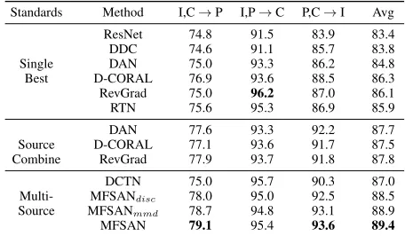
Standards Method I,C→P I,P→C P,C→I Avg

ResNet 74.8 91.5 83.9 83.4

DDC 74.6 91.1 85.7 83.8

Single DAN 75.0 93.3 86.2 84.8

Best D-CORAL 76.9 93.6 88.5 86.3

RevGrad 75.0 96.2 87.0 86.1

RTN 75.6 95.3 86.9 85.9

DAN 77.6 93.3 92.2 87.7

Source D-CORAL 77.1 93.6 91.7 87.5

Combine RevGrad 77.9 93.7 91.8 87.8

DCTN 75.0 95.7 90.3 87.0

Multi- MFSANdisc 78.0 95.0 92.5 88.5

Source MFSANmmd 78.7 94.8 93.1 88.9

MFSAN 79.1 95.4 93.6 89.4

Implementation Details All deep methods are imple-mented base on the pytorch framework, and fine-tuned from pytorch-provided models of ResNet (He et al. 2016). We fine-tune all convolutional and pooling layers and train the classifier layer via back propagation. Since the domain-specific feature extractors and classifiers are trained from scratch, we set its learning rate to be 10 times that of the other layers. We use mini-batch stochastic gradient descent (SGD) with momentum of 0.9 and the learning rate anneal-ing strategy in RevGrad (Ganin and Lempitsky 2015): the

Table 3: Performance Comparison of Classification Accu-racy (%) on Office-Home Dataset.

Standards Method C,P,R A,P,R A,C,R A,C,P Avg

→A →C →P →R

ResNet 65.3 49.6 79.7 75.4 67.5

Single DDC 64.1 50.8 78.2 75.0 67.0

Best DAN 68.2 56.5 80.3 75.9 70.2

D-CORAL 67.0 53.6 80.3 76.3 69.3 RevGrad 67.9 55.9 80.4 75.8 70.0

DAN 68.5 59.4 79.0 82.5 72.4

Source D-CORAL 68.1 58.6 79.5 82.7 72.2 Combine RevGrad 68.4 59.1 79.5 82.7 72.4

MFSANdisc 69.8 60.2 80.2 81.0 72.8

Multi- MFSANmmd 71.1 61.9 79.3 80.8 73.3

Source MFSAN 72.1 62.0 80.3 81.8 74.1

Table 4: Classification Accuracy (%) on Office-31 Dataset for MFSAN with and without disc Loss.

Standards Method A,W →D

A,D →W

D,W →A

Avg

S1 97.7 95.0 68.3 87.0

MFSANmmd S2 85.5 89.0 71.0 81.8

Avg 99.9 98.3 71.5 89.9

S1 97.3 97.6 72.5 89.1

MFSAN S2 96.6 97.7 72.4 88.9

Avg 99.5 98.5 72.7 90.2

learning rate is not selected by a grid search due to high com-putational cost, it is adjusted during SGD using the follow-ing formula:ηp= ₍₁₊η_αp0 ₎β, wherepis the training progress

linearly changing from 0 to 1, η0 = 0.01, α = 10 and β = 0.75, which is optimized to promote convergence and low error on the source domain. To suppress noisy activa-tions at the early stages of training, instead of fixing the adaptation factorλandγ, we gradually change them from

0to1by a progressive schedule:γp=λp= _exp(2_−θp) −1, andθ= 10is fixed throughout the experiments (Ganin and Lempitsky 2015). This progressive strategy significantly sta-bilizes parameter sensitivity and eases model selection for MFSAN.

Results

we compare MFSAN with the baselines on three datasets and the results are shown in Tables 1, 2 and 3, respectively. We also compare the MFSAN with or without disc loss on Office-31 dataset and list the results of each classifier from different sources and the average voting in Table 4. From these results, we have the following insightful observations: • The results of Source Combine are better than Single Best, which demonstrates that combining all source domains into single source domain is helpful in most transfer tasks. This may be due to the data enrichment.

(a) DAN (Single Source): D, A

(b) DAN (Source Com-bine):D, A

(c) DAN (Source Com-bine):W, A

(d) MFSAN:D, A (e) MFSAN:W, A

Figure 3: The Visualization of Latent Representations of Source and Target Domains.

0.01 0.5 1 1.5 2 Number of Iterations(×104₎

60 62 64 66 68 70 72

Accuracy(%)

MFSAN_S1 MFSAN_S2 MFSAN_Avg MFSANmmd_S1

MFSANmmd_S2

MFSANmmd_Avg

(a) Convergence

0.01 0.02 0.05 0.1 0.2 0.5 1 2 λ

65 70 75 80 85 90

Accuracy(%)

D,W→A(MFSAN) I,C→P(MFSAN)

(b) Accuracy w.r.tλ Figure 4: Algorithm Convergence and Parameter Sensitivity.

•Comparing MFSANmmdwith DAN (source combine),

the only difference is that MFSANmmd extracts multiple

domain-invariant representations in multiple feature spaces, while DAN extracts common domain-invariant representa-tions in a common feature space. MFSANmmdis better than

DAN (Source Combine), which shows that it is difficult to extract common domain-invariant representations for all do-mains.

•MFSANdiscoutperforms all compared methods on most

multi-source transfer tasks. This verifies that the consider-ation of the domain-specific class boundary to reduce the gap between all classifiers can help each classifier learn the knowledge from other classifiers.

•Comparing MFSAN with MFSANmmdwhich does not

have disc loss, we find that the results of classifiers from different sources with disc loss (MFSAN) are very close to each other, while there is a large gap between the results of classifiers without disc loss (MFSANmmd). The results

demonstrate the effectiveness of introducing disc loss to re-duce the gap between all classifiers.

Analysis

Feature visualization In Figure 3, we visualize the latent representations of the taskD→Alearned by DAN (Single Source) andD, W→Alearned by DAN (Source Combine), MFSAN using t-SNE embeddings (Donahue et al. 2014).

From Figure 3, we can observe that 1) the results in Fig-ures 3b and 3c are better than the one in Figure 3a, which show that we can benefit from the consideration of more source domains: the results in Figures 3d and 3e are bet-ter than the ones in Figure 3a∼3c, which again validates the effectiveness of our model to align both domain-specific distributions and classifiers.

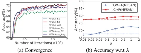
Algorithm Convergence To investigate the convergence our algorithm and the influence of disc loss, we record the performance of MFSAN and MFSANmmd during the

iter-ating on the taskD, W→Ain Figure 4a. We can find that all algorithms can almost converge after1.5×104_iterations.

Also, the results from MFSAN with disc loss have a smaller gap among classifiers and they achieve higher accuracy.

Parameter Sensitivity For simplicity, we set the trade-off parametersλandγas the same value in our experiments, which respectively control the importance of mmd loss and disc loss. To study the sensitivity ofλ, we sample the values in{0.01, 0.02, 0.05, 0.1, 0.2, 0.5, 1, 2}, and perform the ex-periments on tasksD, W→AandI, C→P. All the results are shown in Figure 4b, and we find that the accuracy first increases and then decreases, and displays as a bell-shaped curve. Finally, we setλ= 0.5to achieve good performance.

Conclusion

Most previous deep learning based multi-source domain adaptation methods focus on extracting common domain-invariant representations for all domains without consider-ing domain-specific class boundary. In this paper, we pro-posed a Multiple Feature Space Adaptation Network (MF-SAN), which simultaneously aligns the domain-specific dis-tribution of each pair of source and target domains by learn-ing multiple domain-invariant representations and the out-puts of classifiers from multiple sources. Extensive experi-ments are conducted on three image datasets to demonstrate the effectiveness of the proposed framework. Moreover, our model is a general framework, which can integrate different kinds of mmd loss and disc loss functions.

Acknowledgments

References

Ben-David, S.; Blitzer, J.; Crammer, K.; Kulesza, A.; Pereira, F.; and Vaughan, J. W. 2010. A theory of learning from different domains.Machine learning79(1-2):151–175.

Blitzer, J.; Crammer, K.; Kulesza, A.; Pereira, F.; and Wort-man, J. 2008. Learning bounds for domain adaptation. In

NIPS, 129–136.

Bousmalis, K.; Silberman, N.; Dohan, D.; Erhan, D.; and Krishnan, D. 2017. Unsupervised pixel-level domain adap-tation with generative adversarial networks. InCVPR, vol-ume 1, 7.

Donahue, J.; Jia, Y.; Vinyals, O.; Hoffman, J.; Zhang, N.; Tzeng, E.; and Darrell, T. 2014. Decaf: A deep convolu-tional activation feature for generic visual recognition. In

ICML, 647–655.

Duan, L.; Xu, D.; and Tsang, I. W.-H. 2012. Domain adap-tation from multiple sources: A domain-dependent regular-ization approach.IEEE TNNLS23(3):504–518.

Fernando, B.; Habrard, A.; Sebban, M.; and Tuytelaars, T. 2013. Unsupervised visual domain adaptation using sub-space alignment. InICCV, 2960–2967.

Ganin, Y., and Lempitsky, V. 2015. Unsupervised domain adaptation by backpropagation. InICML, 1180–1189.

Ghifary, M.; Kleijn, W. B.; Zhang, M.; Balduzzi, D.; and Li, W. 2016. Deep reconstruction-classification networks for unsupervised domain adaptation. InECCV, 597–613.

Gong, B.; Shi, Y.; Sha, F.; and Grauman, K. 2012. Geodesic flow kernel for unsupervised domain adaptation. InCVPR, 2066–2073.

Gretton, A.; Borgwardt, K. M.; Rasch, M. J.; Sch¨olkopf, B.; and Smola, A. 2012. A kernel two-sample test. JMLR

13(Mar):723–773.

He, K.; Zhang, X.; Ren, S.; and Sun, J. 2016. Deep residual learning for image recognition. InCVPR, 770–778.

Hoffman, J.; Tzeng, E.; Park, T.; Zhu, J.-Y.; Isola, P.; Saenko, K.; Efros, A. A.; and Darrell, T. 2018. Cycada: Cycle-consistent adversarial domain adaptation. InICML.

Huang, J.; Gretton, A.; Borgwardt, K. M.; Sch¨olkopf, B.; and Smola, A. J. 2007. Correcting sample selection bias by unlabeled data. InNIPS, 601–608.

Jhuo, I.-H.; Liu, D.; Lee, D.; and Chang, S.-F. 2012. Robust visual domain adaptation with low-rank reconstruction. In

CVPR, 2168–2175.

Jiang, J., and Zhai, C. 2007. Instance weighting for domain adaptation in nlp. InACL, 264–271.

Liu, H.; Shao, M.; and Fu, Y. 2016. Structure-preserved multi-source domain adaptation. InICDM, 1059–1064.

Long, M.; Cao, Y.; Wang, J.; and Jordan, M. 2015. Learn-ing transferable features with deep adaptation networks. In

ICML, 97–105.

Long, M.; Zhu, H.; Wang, J.; and Jordan, M. I. 2016. Unsu-pervised domain adaptation with residual transfer networks. InNIPS, 136–144.

Long, M.; Zhu, H.; Wang, J.; and Jordan, M. I. 2017. Deep transfer learning with joint adaptation networks. InICML, 2208–2217.

Mansour, Y.; Mohri, M.; and Rostamizadeh, A. 2009. Do-main adaptation with multiple sources. InNIPS, 1041–1048. Pan, S. J., and Yang, Q. 2010. A survey on transfer learning.

IEEE TKDE22(10):1345–1359.

Pan, S. J.; Tsang, I. W.; Kwok, J. T.; and Yang, Q. 2011. Domain adaptation via transfer component analysis. IEEE TNN22(2):199–210.

Quionero-Candela, J.; Sugiyama, M.; Schwaighofer, A.; and Lawrence, N. D. 2009. Dataset shift in machine learning. The MIT Press.

Ren, S.; He, K.; Girshick, R.; and Sun, J. 2015. Faster r-cnn: Towards real-time object detection with region proposal networks. InNIPS, 91–99.

Saenko, K.; Kulis, B.; Fritz, M.; and Darrell, T. 2010. Adapt-ing visual category models to new domains. InECCV, 213– 226.

Saito, K.; Watanabe, K.; Ushiku, Y.; and Harada, T. 2017. Maximum classifier discrepancy for unsupervised domain adaptation. InCVPR.

Sun, B., and Saenko, K. 2016. Deep coral: Correlation align-ment for deep domain adaptation. InECCV, 443–450. Tzeng, E.; Hoffman, J.; Zhang, N.; Saenko, K.; and Darrell, T. 2014. Deep domain confusion: Maximizing for domain invariance. arXiv preprint arXiv:1412.3474.

Tzeng, E.; Hoffman, J.; Darrell, T.; and Saenko, K. 2015. Simultaneous deep transfer across domains and tasks. In

ICCV, 4068–4076.

Tzeng, E.; Hoffman, J.; Saenko, K.; and Darrell, T. 2017. Adversarial discriminative domain adaptation. In CVPR, volume 1, 4.

Venkateswara, H.; Eusebio, J.; Chakraborty, S.; and Pan-chanathan, S. 2017. Deep hashing network for unsupervised domain adaptation.arXiv preprint arXiv:1706.07522. Xu, R.; Chen, Z.; Zuo, W.; Yan, J.; and Lin, L. 2018. Deep cocktail network: Multi-source unsupervised domain adap-tation with category shift. InCVPR, 3964–3973.

Yang, J.; Yan, R.; and Hauptmann, A. G. 2007. Cross-domain video concept detection using adaptive svms. In

MM, 188–197.

Zhao, H.; Zhang, S.; Wu, G.; Gordon, G. J.; et al. 2018. Mul-tiple source domain adaptation with adversarial learning. In