in the population sciences published by the Max Planck Institute for Demographic Research Konrad-Zuse Str. 1, D-18057 Rostock · GERMANY www.demographic-research.org
DEMOGRAPHIC RESEARCH
VOLUME 24, ARTICLE 29, PAGES 719-748
PUBLISHED 24 MAY 2011
http://www.demographic-research.org/Volumes/Vol24/29/ DOI: 10.4054/DemRes.2011.24.29
Research Article
MAPLES: A general method
for the estimation of age profiles
from standard demographic surveys
(with an application to fertility)
Roberto Impicciatore
Francesco C. Billari
© 2011 Roberto Impicciatore & Francesco C. Billari. This open-access work is published under the terms of the Creative Commons Attribution NonCommercial License 2.0 Germany, which permits use, reproduction & distribution in any medium for non-commercial purposes, provided the original author(s) and source are given credit.
1 Introduction 720
2 The components of MAPLES 721
2.1 Information requirements and data preparation 721 2.2 Estimation and smoothing of age profiles 722
3 Data preparation 723
3.1 Initial dataset and episode-data format 723
3.2 Time-varying variables 725
4 Estimation and smoothing of age profiles 726 4.1 Computation of aggregated events and exposures for any age 726 4.2 Window of observation and episodes 728
4.3 Smoothing procedure 729
5 The MAPLES output 734
5.1 Standard output 734
5.2 The independent hypothesis and the combination of covariates 735
6 An application to Italian GGS data 737
7 Concluding remarks 742
8 Acknowledgments 743
References 744
MAPLES:
A general method for the estimation of age profiles
from standard demographic surveys
(with an application to fertility)
Roberto Impicciatore1
Francesco C. Billari2
Abstract
In this paper we present MAPLES (Method for Age Profiles Longitudinal EStimation), a general method for the estimation of age profiles that uses standard micro-level demographic survey data. The aim is to estimate smoothed age profiles and relative risks for time-fixed and time-varying covariates. MAPLES is implemented through a data processing routine and a series of regressions using GAM (Generalized Additive Models). Although the approach has been developed to be applied for living arrangements and fertility, MAPLES may be used for any kind of life event. In fact, it can be applied to every setting in which micro-level data on transitions are available from a large-scale representative survey (e.g., Demographic and Health Surveys; Fertility and Family Surveys; Generations and Gender Surveys). MAPLES is a R software package containing a set of commands that can be easily applied and that may constitute a useful tool box for demographers and social scientists. The package is available in the CRAN library http://cran.r-project.org/web/packages/MAPLES.
1 Università di Milano. Department of Economics, Business and Statistics, Carlo F. Dondena Centre for Research on Social Dynamics. E-mail: [email protected].
2
1. Introduction
The estimation of smooth age profiles for demographic events from both register and survey data is a problem of general interest, which has triggered a substantial amount of research over the last centuries. Since the earlier works on the “age patterns” of mortality, research has also focused on processes such as fertility and/or marriage. More recently, the estimation of age profiles has then been naturally embedded within the event history framework, making room for the role of time-constant and time-varying covariates in regression models. Furthermore, several models that minimize the strength of the assumption on the shape of the underlying age profiles have been proposed and used. An example is the fertility model by Schmertmann (2003) based on splines. The interpolation of age profiles through splines had been proposed earlier by McNeil, Trussel, and Turner (1977).
When the interest is not on a single transition, but on a multistate set of transitions, the need for a general and consistent method for the estimation of age profiles becomes even more evident. This is crucial, for instance, when developing multistate population forecasts, i.e. when forecasts are developed in order to account for the complexity of life course trajectories. A typical example is the need to forecast individuals according to statuses such as living arrangement and number of children. This is the approach, for instance, of the “MicMac” population forecasting framework, which aims at explicitly taking into account the life course trajectories of individuals in population forecasts (see e.g., Willekens 2005; van der Gaaget al. 2006). The life course is viewed as a sequence of states and events; each event marks a transition from one state to another (see also the statistical approach developed in Andersen et al. 1993). The study of a single transition is based on the estimation of its transition rates (from the original state to the destination state, in a defined state space). From the literature on living arrangements and fertility, we know that these behaviours are strongly related to age. Indeed, such variation with age has traditionally been exploited in demographic forecasting.
e propose.
transition, even for small subgroups of a population (e.g. highly educated women living in a specific region with one child and divorced). We present the model also by developing a specific application to the data of the Italian Generations and Gender Survey (GGS).
This paper is structured as follows: In section 2 we introduce the basic components of MAPLES; in section 3 we discuss the approach to data preparation; in section 4 we enter into the details of the method by showing the procedure used to aggregate events and exposures and the smoothing algorithm; in section 5 we illustrate the output of MAPLES and in section 6 we show and discuss an application to the Italian GSS data. Finally, section 7 contains some concluding remarks about the limits and the advantages of the method.
2. The components of MAPLES
MAPLES has been developed to obtain a flexible method that can be applied in different contexts and in every setting in which relatively standard longitudinal data are available from a representative survey. In addition, the method can explicitly take into account the interactions between different life course trajectories, through the inclusion of both time-constant and time-varying covariates. Being based on regression models, the method also permits us to test hypotheses. The whole method is implemented in the publicly available R software, and it can easily be recalled as an R package in order to be applied to user-provided data.3 Let us start by giving a step-by-step description of the basic components of MAPLES, i.e. data preparation and age-profile estimation. In the following sections we will detail each step and also take advantage of the application w
2.1 Information requirements and data preparation
MAPLES requires, as input, the same information used in the popular “counting process” formulation of survival analysis (see e.g. Andersen et al. 1993). Each record in the dataset has to contain three variables describing the survival time: a start variable specifies when observation begins; a stop variable specifies when it ends; and a status indicating if the episode ends with an event or not. Thedata structure, sometimes called
episode-data structure (see among others Blossfeld and Rowher 2002), is automatically
created by the command epdata in the MAPLES package. Therefore, assuming that we have a dataset which contains the dates of the events of interest, recorded either in years (on a continuous time axis) or in CMC (century month code), and a set of covariates, the command epdata creates a new dataset that can be promptly used in MAPLES as well as other R packages such as survival (Therneau 1999; Lumley 2004). Moreover, in the resulting dataset we may add a set of time-varying variables by splitting the original episode in two or more sub-episodes and then allowing one or more variables to change over the spell. This operation is achieved through the
splitter command in the MAPLES package.
2.2 Estimation and smoothing of age profiles
The core of MAPLES is the command ageprofile. The estimation process consists in two main steps:
1. Computation of aggregated events and exposures for any age. The “micro-data” structure (one row = one individual) is transformed into a multistate “macro-data” structure (one row = one combination of age and levels of covariates). The number of events and exposures may be restricted in various ways according to the needs of the researcher: to a specific window of observation defined as a calendar window (e.g. in the last 10 years before the interview; between 2000 and 2005; etc.); between two ages (e.g. between 20 and 25 years of age); between two relevant events in the life course (e.g. between marriage and the first child; between the divorce and the interview). The specification of a window of observation defined as the latest available period (e.g. the last 5 years before the interview) is particularly interesting when age profiles are used in population projections (Impicciatore and Billari 2007).
3. Data preparation
We now focus on the steps of the data preparation procedure.
3.1 Initial dataset and episode-data format
A generic transition represents the passage from state A to state B marked by the experience of an event EAB. Therefore, a transition is well defined when we know which event causes it, at which point in time it occurs and when the individual starts to be at
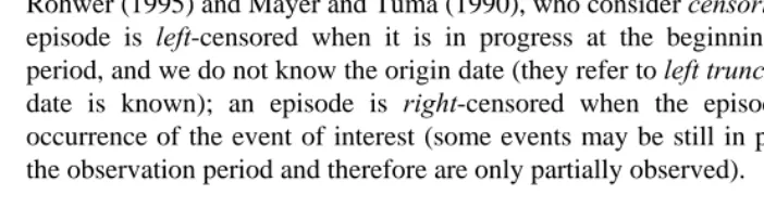
risk of experiencing this event. Moreover, at a certain point in time an individual may undergo an event that does not permit us to follow his/her life course further on, i.e. the observation is censored (Blossfeld and Rowher 2002). With retrospective survey data, right censoring might be induced by the interview or might occur at another specific point in time. For example, if we are studying the transition to divorce for married people, right censoring can occur at the death of spouse. Left censoring might arises in retrospective surveys when individuals are asked to report the states they occupy at the date of the survey and only up to some time prior to that date. As an example, we may consider the case where individuals were asked to declare their occupation at the time of the interview and their occupational trajectory during the last 5 years (D’Addio and Rosholm 2002). In the latter case, the real origin date of a spell, i.e. when the individual starts to be at risk, is unknown. We here follow the perspective used by Blossfeld and Rohwer (1995) and Mayer and Tuma (1990), who consider censoring symmetrically: an episode is left-censored when it is in progress at the beginning of the observation period, and we do not know the origin date (they refer to left truncation when the origin date is known); an episode is right-censored when the episode ends without the occurrence of the event of interest (some events may be still in progress at the end of the observation period and therefore are only partially observed).
Table 1: Record structure in the initial dataset
1 identification number (individual level) optional
2 normalized weight optional
3 date at the beginning of the episode alternative to 6 4 date at event of interest alternative to 7
5 date at birth mandatory
Formally, we define the episode for the j-th individual as the time interval between S
tj (the point in time when the individual enters into state A, i.e. starts to be at risk of experiencing EAB, or when the observation is left censored) and tFj (the point in time when EABoccurs or when the observation is right censored).
Focusing on a single transition, we need the basic information specified in table 1 in order to apply MAPLES. We assume that when the date of right censoring is available, the date of the event is missing. Symmetrically, when the date of left censoring is available, the date at the beginning of the episode is missing. The individual birth date is used to compute the age at the beginning and at the end of the episode. All dates must be either in years or in CMC (century month code). Since very often survey data contains information in the format of month and year, we can easily transform the date of a generic event in a continuous expression through the formula:
month 0.5 date_event_years year 1900
12
−
= − + (1)
Note that a date is pointed to the middle of the specified month. Alternatively, CMC may be computed as4:
date_event_cmc=(year 1900) 12− ⋅ +month (2)
In any case, the corresponding age at the specific event is computed as:
age=date_event-date_birth (3)
where date_birth is the decimal date of birth.
Through the epdata command, the initial dataset, as specified in table 1, can be transformed in the episode-data format shown in table 2.
The new variable status indicates whether the episode is right censored and/or left censored. Following the same approach used in the R package survival (Therneau 1999; Lumley 2004), this variable is 0 when the episode is right censored; 1 if the event occurred; 2 if the event occurred and the episode is left-censored; 3 if the episode is double censored (interval censored). See figure 1 for a graphic representation of these variables. The variable status is computed according to the availability of relevant dates: if the date of an event is missing, we assume that the event has not been experienced before the end of the episode. Besides, a non-missing left-censoring date changes the value of the status variables. These rules strictly require that unknown dates
are not written as “missing” in the initial dataset. This is in line with indications given by other authors. For example, Matsuo and Willekens (2003) specify that a missing year means that the event did not occur even when the respondent indicated, in another item, that the event did occur. Therefore, the user must pay attention to missing values in the dataset, check possible missing dates and exclude ambiguous cases from the dataset.
Table 2: Record structure in the episode dataset
Variable name description
id identification number (individual level) Tstart date at the beginning of the episode Tstop date at the end of the episode
status variables that indicates if the episode ends with an event agestart individual age at Tstart
agestop individual age at Tstop birth date of birth
…. user-defined covariates
The resulting episode dataset (epdata file from now on) can be used without further changes in other R packages, and in particular in survival (Therneau 1999; Lumley 2004).
Figure 1: Record structure in the episode dataset
3.2 Time-varying variables
Information on a time-varying variable is carried over by “splitting” the individual episode at the point the change occurs (see Blossfeld and Rohwer 2002). Each sub-episode resulting from splitting is characterized by a unique value of the time-varying variable. For example, let us consider the transition from married to divorce. An episode that ends with divorce may be described by a vector of four values (tSj,
F j
t , 0, 1) describing, respectively, the starting time, the final time, the starting status (0 as married) and the final status (1 as divorced). We can also suppose that at times tCHj 1 and
2 CH j
t (where tSj< 1 CH j
t < CH2 j
t < tF
j ) the j-th individual experienced the birth of the first and second child respectively. The original episode is thus split into the three sub-episodes: (tSj, , 0, 0), (
1 CH j
t , CH2 j
t , 0, 0) , and ( CH2 1
CH j
t tj ,
F j
t , 0, 1). The (time-varying) covariate “number of children” is fixed at 0 (childless) in the first sub-episode, at 1 in the second and at 2 in the third. This may be repeated for each potential time-varying variable. Episode splitting is performed through the command splitter applied to an
epdata dataset. The resulting dataset preserves the same record structure of the input data, even though we may have more than one record for the same individual.
4. Estimation and smoothing of age profiles
4.1 Computation of aggregated events and exposures for any age
t-th calendar year. Therefore, they refer to two different years of age (in completed years) x-1 and x. Cohort-period rates are particularly helpful in demographic projections using a cohort-component approach. MAPLES can estimate age profiles using both cohort-age and cohort-period rates.
Figure 2: Area of interest in the Lexis diagram according to the kind of rate
a. Cohort-age rate b. Cohort-period rate
The transition rate at age x (ratex) is the ratio between the number of events OCCx and the amount of time spent in the initial state EXPx collected respectively in ABCD for the cohort-age classification and in AEBD for the cohort-period classification (see fig. 2).
In order to show how events and exposures can be computed using longitudinal data, let us consider a generic j-th episode
(
t tSj, Fj)
and the associate (exact) age interval(
xSj,xFj)
. Let us also assume that each episode has an assigned post-stratification sampling weight equal to w(j). Following the cohort-age perspective, the number of occurrences and exposures at any age x (in completed years) and for each combination of covariate levels z (for factor covariates), are respectively:, ,
1
, ,
1
OCC occ ( )
EXP exp ( )
N
x z x z
j N
x z x z
j
j w
j w
=
=
= ⋅
= ⋅
∑
∑
( )
( )
j
j
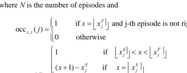
where N is the number of episodes and
,
1 if and j-th episode is not right-censored occ ( )
0 otherwise F j x z
x x
j = ⎨⎧⎪ =⎢ ⎥⎣ ⎦
⎪⎩ (5)
,
1 if
( 1) if
exp ( )
if
0 if or
S F
j j
S S
j j
x z F F
j j
S F
j j
x x x
x x x x
j
x x x x
x x x x
⎧ ⎢ ⎥⎣ ⎦< <⎢⎣ ⎥⎦
⎪ ⎪ + − =⎢ ⎥ ⎪ ⎣ ⎦ = ⎨ ⎢ ⎥ − = ⎪ ⎣ ⎦ ⎪ ⎢ ⎥ ⎢ ⎥
⎪ <⎣ ⎦ >⎣ ⎦
⎩
(6)
where ⌊y⌋ is the largest integer less than or equal to y. For example, let us suppose that a generic uncensored episode starts at the exact age xS = 39.31 and ends at the exact age
xF =
43.83. The number of occurrences for this episode is 1 at age (in completed years)
x = 43 and 0 at any other ages; the contribution to the number of exposures is 0.69 at x = 39, 1 at x = 40, 41, 42 and 0.83 at x = 43.
The resulting data matrix contains in each row the number of occurrences and exposures for any combination of age and levels of covariates. For example, if we consider an age range from 15 to 69 (55 age classes) and level of education as a covariate with 6 levels, the matrix will have 330 rows (among them, rows with zero exposure time will be dropped from the matrix).
This procedure can be extended to the cohort-period perspective under the assumption that the rate at age x is the rate at time t that considers events in AEBD (see figure 2b) and covering age x-1 and x.5
4.2 Window of observation and episodes
In demography, rates computed with macro-data usually refer to a specific calendar period (one or two years in most cases). Using longitudinal micro-data we do not have an unambiguous calendar period of reference. Therefore, it may be useful to restrict the computation of events and exposures to a specific and user-defined period. This period, which we call window of observation, may be defined not only as the period between
two calendar dates (fixed for the whole sample or specific for every individual) but also through any other two points in time specific for each individual (e.g. between two ages, two events, etc.). Generally speaking, for the j-th individual the window of observation is the user-defined time interval
(
WINj stop)
start WIN
j t
t _ _
, . Events and exposures will be counted only within this window of observation. Thus, all the episodes with a null intersection with the relative window of observation will be excluded.
4.3 Smoothing procedure
If we consider the transition rate for a specific event as the dependent variable, we should model it as a function of age and a set of covariates. However, age profiles for a specific transition should never be considered as a linear function. The smoothing or graduation of rates, or more specifically the age profile of rates, has been a traditional issue in various disciplines, including demography and actuarial sciences. Approaches based on various kinds of polynomial functions have been criticized in the literature for a long time. Some scholars proposed the use of spline functions as a solution (see e.g., McNeil, Trussell, and Turner 1977). More recent developments include Smith, Hyndman, and Wood (2004), and the study on age-specific fertility rates by Schmertmann (2003).
For our purpose, the so-called family of Generalized Additive Models provides a suitable solution (Hastie and Tibshirani 1990; Chambers and Hastie 1992; Hastie, Tibshirani, and Friedman 2001), also for the framework that naturally allows for the inclusion of covariates. GAMs constitute a generalization of linear regression models where the dependent variable Y can be modelled as a sum of non-linear (smoother) functions.
The model structure is as follows:
∑
+ +
=
k kX age
f
g(μ) β0 ( ) β k (7)
Since transition rates at age x for a specific event are given by the ratio between number of events (OCC) and the time of exposure (EXP), considering the natural logarithm as link function, for each i-throw of data matrix6 we can write:
0 1
OCC
ln ( )
EXP i
i i
i
f age Z i
β β ε
⎛ ⎞
= + + +
⎜ ⎟
⎝ ⎠ (8)
and
0 1
ln(OCC )i =ln(EXP )i +β + f age( i)+βZi+εi (9)
where εi is a random error term, OCC~ Poisson and the term ln(EXP) has no coefficient to be estimated (i.e. it is an offset).
In our dataset, OCCi are calculated starting from individual weighted information. As a consequence, the number of events and the time of exposure are not integers. Since the Poisson distribution is defined only for integers, we need to round the number of weighted events. Empirical robustness checks (not shown here) suggest that this approximation is acceptable.
The smoothing function f is a piecewise cubic spline, a curve made up of sections of cubic polynomial joined together so that they are continuous in value, as well as first and second derivatives. The points at which the sections join are known as the knots of the spline that are placed at quantiles of the distribution of unique x values. The number of knots defines the degree of smoothness of the f (i.e. number of knots + 2). In order to avoid the choice of the number of parameters, which is essentially arbitrary, the degree of smoothness is estimated by Generalized Cross Validation7 (Wood 2006).
The effect of covariates is considered as a multiplicative change to be applied to the grand mean, i.e. to the mean risk for the whole sample. This is pursued by applying the “deviation coding” system that compares the mean of the dependent variable for a given level to the overall mean of the dependent variable. We now focus as an example on educational level. We report an example of deviation coding for four educational levels in table 3.
6 We remember that each row of the data matrix is given by a specific combination of age x and the levels of a factor covariate (or a combination of factor covariates).
Table 3: Deviation coding. An example for education (with 4 levels)
EDU Dummy 1
(Primary vs. mean)
Dummy 2 (Low. sec. vs mean)
Dummy 3 (Upp. sec vs mean)
Primary 1 0 0
Lower secondary 0 1 0
Upper secondary 0 0 1
Tertiary -1 -1 -1
Since the expected values of the dummy variables in deviation coding are always zero8, we can obtain the baseline age profile, or grand mean transition rates, as:
) i age ( 0 f i e
baseline = β+
. (10)
Following the deviation coding system, the relative risks for level of education are:
1 2 3 1 2 ("primary") ("low sec") ("upp sec") 1 ("tertiary") rrisk e rrisk e rrisk e rrisk e β β β 3 β β β+ + = = = = (11)
The transition rate at age x for a specific level, for example, primary level of education, is then:
("primary") ("primary")
x x
rate =baseline rrisk⋅ (12)
The estimated coefficients express multiplicative changes that must be applied at the baseline age profile in order to evaluate the estimated risk for each year of age. In other words, the effect of a covariate can be seen as a vertical shift throughout the whole range of ages. In the implementation we propose, the user can decide to apply multiplicative change to the baseline only if the difference between the level considered and the grand mean is statistically significant at a user-defined level (95% by default), i.e. if the coefficient β is significantly different from zero with an associate p-value lower than the user-defined value (0.05 by default).
Figure 3: Multiplicative effects of covariates estimated with additive model. Effects of education on first marriage. Italy. GGS 2003
Figure 3 shows an example of multiplicative effect by level of education on the transition to first marriage. Since very often the effect of a covariate combines vertical and horizontal shifts, the proportional assumption on the whole age rank appears too simplistic. MAPLES adopts the following solution: the multiplicative effect of a covariate is estimated separately within three different sub-intervals of ages. These intervals are obtained by fixing two knots at the 33rd and 67th percentiles of the cumulative distribution of the unsmoothed occurrence-exposures estimated at each age
x using expression (4). With this new configuration, the model contains, other than the baseline transition rate, given as a function of age, a set of 3*m dummy variables in which m is the number of factor levels and 3 is the number age sub-intervals. In order to improve the goodness of fit, the knots may be computed separately for each level of a covariate. Therefore, the effect of each specific level is estimated by applying the GAM model as stated above for each pair of knots.
Figure 4: Proportional effects of education on first marriage. Italy. GGS 2003
Figure 5: Smoothed curves. Effects of education on first marriage. Italy.
5. The MAPLES output
5.1 Standard output
The final output of MAPLES consists of a list of elements:
• a matrix containing (in column) the baseline age profile (achieved through the estimation of a model without covariates) and a set of vectors containing age profiles for every level of all the covariates specified by the user.
• a matrix of unsmoothed age profiles, i.e. transition rates as a ratio between aggregated events (OCC) and exposures (EXP) as computed in (4).
• a matrix with all the pairs of knots (column) for any level (row);
• a matrix with the number of weighted events classified by age subinterval (column) and covariate levels (row);
• a matrix of relative risks estimated through GAM models by age subinterval (column) and covariate levels (row);
• a matrix of standard errors for relative risks estimated by GAM models according to age subinterval (column) and covariate levels (row);
• a matrix of p-values estimated by GAM models by age subinterval (column) and covariate levels (row);
• a vector of p-values, one for each covariate X, related to the comparison between a model without X and model with X. The fitted models are compared using an analysis of deviance table. The tests are usually approximated, unless the models are un-penalized (Wood 2006).
5.2 The independent hypothesis and the combination of covariates
MAPLES can handle any number of covariates, but covariate effects are estimated separately. Therefore, under the independence hypothesis, transition rates for a subsample defined by a specific combination of covariates can be easily computed as products of relative risks for each single level and the relative baseline. For a given transition, we can define ratex(c1, c2, c3,…) asthe transition rate at age x for individuals with values c1, c2, c3,… respectively for covariates C1, C2, C3,… Hence, we find that:
1 2 3
1 2 3
( ) ( ) ( )
( , , ,...) x x x ...
x x
x x x
rate c rate c rate c rate c c c baseline
baseline baseline baseline
= ⋅ ⋅ ⋅ ⋅ (22)
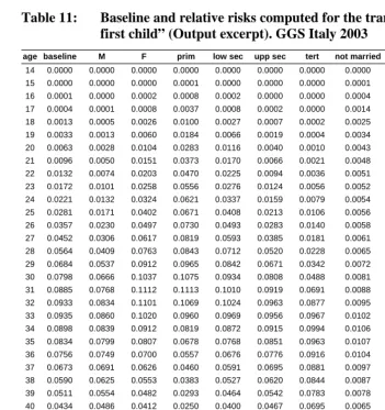
where baselinex is the transition rate at age x estimated in the model without covariates and ratex(ci) is the transitioin rate at age x estimated for a specific level of the i-th covariate, i.e. when Ci= ci. Following the example shown in table 11, we want to know the estimated transition rates to first child for women aged x=30 with a tertiary level of education, in the second marriage.
The application of MAPLES gives us the following rates:
(
)
(
)
(
)
30
30
30
30
0.0798 ="F" 0.1037 ="tertiary" 0.0488 ="2nd marr" 0.4573
baseline rate sex rate edu rate mar
= = = =
The required rate is, then:
30
0.1037 0.0488 0.4573 ( "F", "tert ", "2nd marr ") 0.0798
0.0798 0.0798 0.0798 0.3634
rate sex= edu= mar= = ⋅ ⋅ ⋅
Table 11: Baseline and relative risks computed for the transition “Childless - first child” (Output excerpt). GGS Italy 2003
age baseline M F prim low sec upp sec tert not married 1st marr wid/div 2nd marr
14 0.0000 0.0000 0.0000 0.0000 0.0000 0.0000 0.0000 0.0000 0.0004 0.0001 0.0008 15 0.0000 0.0000 0.0000 0.0001 0.0000 0.0000 0.0000 0.0001 0.0021 0.0004 0.0141
16 0.0001 0.0000 0.0002 0.0008 0.0002 0.0000 0.0000 0.0004 0.0097 0.0017 0.0871
17 0.0004 0.0001 0.0008 0.0037 0.0008 0.0002 0.0000 0.0014 0.0383 0.0067 0.1829
18 0.0013 0.0005 0.0026 0.0100 0.0027 0.0007 0.0002 0.0025 0.1123 0.0209 0.2868
19 0.0033 0.0013 0.0060 0.0184 0.0066 0.0019 0.0004 0.0034 0.2226 0.0470 0.3947
20 0.0063 0.0028 0.0104 0.0283 0.0116 0.0040 0.0010 0.0043 0.3171 0.0760 0.4850
21 0.0096 0.0050 0.0151 0.0373 0.0170 0.0066 0.0021 0.0048 0.3658 0.0957 0.5372
22 0.0132 0.0074 0.0203 0.0470 0.0225 0.0094 0.0036 0.0051 0.3725 0.1034 0.5474
23 0.0172 0.0101 0.0258 0.0556 0.0276 0.0124 0.0056 0.0052 0.3548 0.1023 0.5282 24 0.0221 0.0132 0.0324 0.0621 0.0337 0.0159 0.0079 0.0054 0.3249 0.0975 0.4968
25 0.0281 0.0171 0.0402 0.0671 0.0408 0.0213 0.0106 0.0056 0.2970 0.0914 0.4670
26 0.0357 0.0230 0.0497 0.0730 0.0493 0.0283 0.0140 0.0058 0.2758 0.0868 0.4463
27 0.0452 0.0306 0.0617 0.0819 0.0593 0.0385 0.0181 0.0061 0.2632 0.0844 0.4367
28 0.0564 0.0409 0.0763 0.0843 0.0712 0.0520 0.0228 0.0065 0.2583 0.0841 0.4369
29 0.0684 0.0537 0.0912 0.0965 0.0842 0.0671 0.0342 0.0072 0.2593 0.0854 0.4463
30 0.0798 0.0666 0.1037 0.1075 0.0934 0.0808 0.0488 0.0081 0.2635 0.0875 0.4573
31 0.0885 0.0768 0.1112 0.1113 0.1010 0.0919 0.0691 0.0088 0.2678 0.0895 0.4669 32 0.0933 0.0834 0.1101 0.1069 0.1024 0.0963 0.0877 0.0095 0.2658 0.0903 0.4713
33 0.0935 0.0860 0.1020 0.0960 0.0969 0.0956 0.0967 0.0102 0.2587 0.0894 0.4676
34 0.0898 0.0839 0.0912 0.0819 0.0872 0.0915 0.0994 0.0106 0.2440 0.0863 0.4546
35 0.0834 0.0799 0.0807 0.0678 0.0768 0.0851 0.0963 0.0107 0.2234 0.0811 0.4335
36 0.0756 0.0749 0.0700 0.0557 0.0676 0.0776 0.0916 0.0104 0.2001 0.0744 0.4074
37 0.0673 0.0691 0.0626 0.0460 0.0591 0.0695 0.0881 0.0097 0.1763 0.0667 0.3530
38 0.0590 0.0625 0.0553 0.0383 0.0527 0.0620 0.0844 0.0087 0.1519 0.0585 0.3024 39 0.0511 0.0554 0.0482 0.0293 0.0464 0.0542 0.0783 0.0078 0.1299 0.0501 0.2448
40 0.0434 0.0486 0.0412 0.0250 0.0400 0.0467 0.0695 0.0065 0.1085 0.0420 0.1860
41 0.0361 0.0408 0.0342 0.0207 0.0334 0.0393 0.0599 0.0053 0.0885 0.0343 0.1345
42 0.0291 0.0332 0.0275 0.0166 0.0269 0.0320 0.0481 0.0041 0.0704 0.0273 0.0950
43 0.0228 0.0262 0.0213 0.0129 0.0208 0.0252 0.0374 0.0032 0.0545 0.0211 0.0670
44 0.0172 0.0198 0.0159 0.0097 0.0156 0.0191 0.0282 0.0024 0.0410 0.0159 0.0443
45 0.0127 0.0144 0.0116 0.0071 0.0114 0.0140 0.0207 0.0018 0.0302 0.0117 0.0322
46 0.0091 0.0102 0.0082 0.0052 0.0082 0.0100 0.0150 0.0013 0.0218 0.0085 0.0230
47 0.0064 0.0071 0.0058 0.0037 0.0058 0.0071 0.0107 0.0009 0.0155 0.0060 0.0162 48 0.0045 0.0048 0.0040 0.0027 0.0042 0.0050 0.0077 0.0007 0.0109 0.0043 0.0114
49 0.0031 0.0033 0.0028 0.0019 0.0030 0.0036 0.0055 0.0005 0.0077 0.0030 0.0080
There are a number of cases in which it is interesting to evaluate the joint effect of some covariates on the transition rate. In order to relax the hypothesis that covariates have an independent effect (and therefore can be combined through multiplication), we can run MAPLES introducing an interaction variable, i.e. a variable that is the combination of two or more variables. For example, instead of specifying the two variables, sex and level of education, as separate covariates with 2 (M and F) and 4 (prim, lowsec, upp sec, tertiary) levels each, respectively, we may introduce the interaction with 8 levels (M_prim, M_lowsec, M_uppsec, M_tert, F_prim, F_lowsec, F_uppsec, F_tert).
6. An application to Italian GGS data
We conclude the paper by describing an application to Italy. Data come from the multi-purpose survey called “Famiglia e soggetti sociali”, that is associated with the Generations and Gender Programme (Vikat et al. 2007). Carried out at the end of 2003, this survey contains wide retrospective information on life course trajectories and transition to adulthood, including data on the history of marital unions, cohabitations (followed by a marriage or not) and marital disruption, for a large sample of the resident population aged 18 or more at the interview.
Our application focuses on the transition to the first child. We also want to highlight differences according to the following variables:
1. area of residence at the interview (time-fixed): North, Central, South; 2. current marital status (time-varying): married, not married;
3. level of education at the interview (time-fixed): lower secondary or lower level, upper secondary level, tertiary level.
The input dataset contains the following information (in cmc or continuous format, see formulas 1 and 2):
• date of the event that caused the entry into the period at risk, i.e. when the episode began (14th birthday);
• date of the transition (first child), if any;
• date of events that imply the exit from observation, i.e. right censoring (interview); • date at first marriage (in order to define the current marital status), if any;
Missing values in the date at first childbirth and date at marriage mean that the relative event has not been experienced till the interview. Therefore, the user should check data to detect inconsistencies. Generally speaking, focusing on dates, we can find inconsistencies that may remain hidden otherwise. For example, some sequences of dates cannot be real (e.g. second marriage experienced before the end of first marriage, second child born before first child) and the occurrence of other events may be revealed even though the date is missing (e.g. the end of first marriage is missing but we know that it occurred given that the date of second marriage is reported). Inconsistent sequencing and/or timing of events may be due to typing errors made by interviewer or during the data capture. The user should use all available information in order to correct these inconsistencies before proceeding with age profile estimation. Our approach has been to drop the case when an inconsistent date is detected.
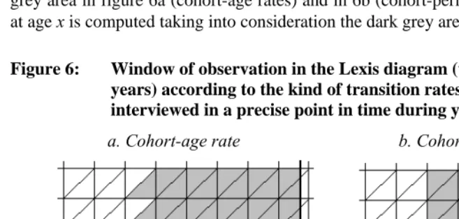
Let us suppose that we are interested in the estimation of age profiles for forecasting purposes (see Willekens 2005). In this case, we may be interested only in the most recent behaviours experienced by Italian people, e.g. the last five years before the interview (1998-2003). The window of observation in the Lexis diagram is the light grey area in figure 6a (cohort-age rates) and in 6b (cohort-period rates). Transition rate at age x is computed taking into consideration the dark grey area.
Figure 6: Window of observation in the Lexis diagram (window length = 5
years) according to the kind of transition rates. Individuals are interviewed in a precise point in time during year t
We apply the command epdata in order to transforms the initial dataset in an
epdata file (episode-data format). The time-varying variable “marital status” is implemented by splitting the resulting dataset through the command splitter. The next step is the computation of age profiles. Since we are interested in population projections, we focus on cohort-period rates. As a first attempt we can run the command
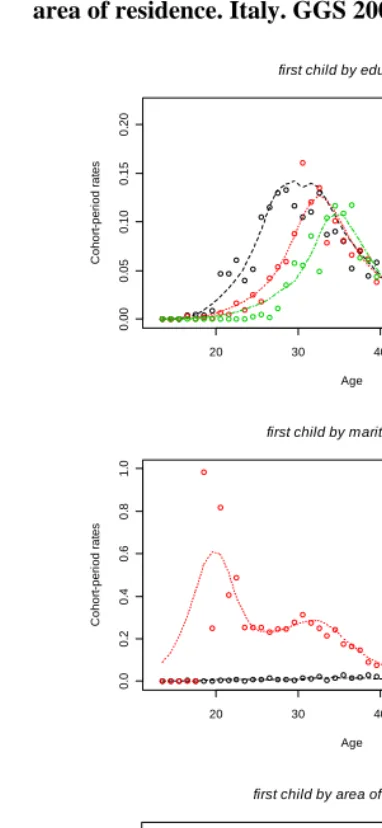
ageprofile taking the three covariates (area, education, marital status) as independent, i.e. we evaluate the age profile for each level separately of each covariate. The graphical output, obtained through the command plotap, is shown in figure 7. The curves represent the estimated age profiles and the points are the unsmoothed occurrence-exposure rates estimated at each age x using expression (4). The points also coincide with the estimates of the hazard rates obtained through the application of the Kaplan Meier method using the survival package.
Figure 7: Estimated transition rates for the first childbirth. Age profiles for women according to level of education, current marital status and area of residence. Italy. GGS 2003
20 30 40 50 60
0. 0 0 0. 05 0 .10 0. 1 5 0. 20 Age C o h o rt -p e ri o d r a te s
first child by education
low sec upp sec tert
20 30 40 50 60
0. 0 0. 2 0. 4 0 .6 0 .8 1 .0 Age C o h o rt -p e ri o d r a te s
first child by marital status
not marr marr
20 30 40 50 60
0. 00 0. 05 0. 10 0 .15 0. 2 0 Age C oho rt -per iod r a tes
first child by area of residence
Figure 8: Estimated transition rates for the first child birth. Age profiles for women according to the interaction between level of education and area of residence. Italy. GGS 2003
20 30 40 50 60
0. 00 0. 05 0. 10 0. 15 0. 20 Age C o hor t-per io d r at es
first birth by education - NORTH
lowsec-N uppsec-N tert-N
20 30 40 50 60
0. 00 0. 05 0. 10 0 .15 0. 2 0 Age C oho rt -per iod r a tes
first birth by education - CENTRAL
lowsec-C uppsec-C tert-C
20 30 40 50 60
0 .0 0 0. 05 0. 10 0. 15 0. 20 Age C o h o rt-p e ri o d ra te s
first birth by education - SOUTH
Figure 9: Estimated transition rates for the first child birth. Age profiles for women with tertiary level of education according to area of residence. Italy. GGS 2003
20 30 40 50 60
0.
0
0
0
.05
0.
1
0
0
.15
0.
2
0
Age
C
o
hor
t-pe
ri
od
r
at
es
first birth - women with tertiary level by area
tert-N tert-C tert-S
7. Concluding remarks
In this paper we presented MAPLES (Method for Age Profiles Longitudinal EStimation), a general method for the estimation of age profiles that uses standard micro-level demographic survey data such as Demographic and Health Surveys, Fertility and Family Surveys or Generation and Gender Survey. The method, and its related computer program written in R, is tailored for the computation of occurrence-exposure rates for any kind of transition among states taking into account the effect on the age profile of time-constant and time-varying covariates. MAPLES has been developed with the aim to obtain a flexible method that can be applied in different contexts and in every setting in which relatively standard longitudinal data are available from a representative survey.
MAPLES, as one would expect, also has some limitations, and there is room for further development and extension of the method. First, the covariates that we can implement are only nominal, or factor variables (i.e. variables with a limited number of categories), so both ordinal and continuous variables have to be converted to nominal variables. Secondly, the transition rates refer to a specific age, regardless the time spent in the initial state for each individual. In other words, we cannot handle duration dependence within our method.
micro-simulation. However, it could be also useful as a descriptive tool in the analysis of specific transitions among different states and population subgroups. One of the most important advantages of the method we propose is the possibility of estimating the age pattern for small subgroups e.g. highly educated women living in a specific region with one child and divorced. In order to do so, for instance, the method estimates the age profile by “anchoring” it to the baseline estimated for the whole sample.
8. Acknowledgments
References
Andersen, P.K., Borgan, Ø., Gill, R.D., and Keiding, N. (1993). Statistical Models
Based on Counting Processes. Berlin and New York: Springer.
Blossfeld, H.-P. and Rohwer, G. (2002). Techniques of Event History Modelling. Mahwah, NJ: Lawrence Erlbaum Associates.
Chambers, J.M. and Hastie, T.J. (eds.) (1992). Statistical models in S. New York: Chapman and Hall.
D’Addio, A.C. and Rosholm, M. (2002). Left-censoring in duration data: Theory and applications. Department of economics, University of Aarhus, Denmark. (Working Paper No. 2002-5).
Hastie, T.J. and Tibshirani, R.J. (1990). Generalized additive models. London: Chapman and Hall.
Hastie, T.J., Tibshirani, R.J., and Friedman, J. (2001). The elements of statistical
learning. Data mining, inference and prediction. New York: Springer-Verlag. Impicciatore, R. and Billari, F.C. (2007). Age profile estimation for family and fertility
events based on micro data: The MAPLE (Method for age profile longitudinal estimation). In: EUROSTAT methodologies and working papers. Bucharest: Joint Eurostat-UNECE work session on demographic projections: 77-98.
Lumley, T. (2004). The survival package. The newsletter of the R project 4/1(June): 26-28.
Matsuo, H. and Willekens, F. (2003). Event histories in the Netherlands Fertility and Family Survey 1998: A technical report. Groningen: Population Research Centre, University of Groningen. (PRC Research Report 2003-1).
Mayer, K.U. and Tuma, N.B. (eds.). (1990). Event history analysis in life course
research. Madison: University of Wisconsin Press.
McNeil, D.R., Trussell, T.J., and Turner, J.C. (1977). Spline interpolation of demographic data. Demography 14(2): 245-252. doi:10.2307/2060581.
Smith, L., Hyndman, R.J., and Wood, S.N. (2004). Spline interpolation for demographic variables: The monotonicity problem. Journal of Population
Research 21(1): 95-98. doi:10.1007/BF03032212.
Therneau, T.M. (1999). A package for survival analysis in S. [http://citeseerx. ist.psu.edu/viewdoc/download?doi=10.1.1.126.7246&rep=rep1&type=pdf]. The survival package is available in the CRAN library: http://cran.r-project.org/ web/packages/survival/index.html.
van der Gaag, N., de Beer, J., Ekamper, P., and Willekens, F. (2006). Using MicMac to
project living arrangements: an illustration of biographic projections. Paper presented at the European Population Conference, Liverpool.
Vikat, A., Spéder, Z., Beets, G., Billari, F.C., Buhler, C., Désesquelles, A., Fokkema, T., Hoem, J., MacDonald, A., Neyer, G., Pailhé, A., Pinnelli, A., and Solaz, A. (2007). Generations and Gender Survey (GGS): Toward a better understanding of relationship and processes in the life course. Demographic Research 17(14): 389-440. doi:10.4054/DemRes.2007.17.14.
Willekens, F. (2005). Biographic forecasting: Bridging the micro-macro gap in population forecasting. New Zealand Population Review 31(1): 77-124.
Appendix
A. Smoothing procedure based on logistic weights
Let us consider the interval of age that starts at the midpoint of the first subinterval (point A in figure A.1: age at which at least 16% of the events have been experienced) and ends at the middle point of the second sub-interval (point B: median age). At point
A, the transition rate is the product of the baseline at A by the relative risk associated with the covariate level for the first sub-interval (β1). At point B the transition rate is the baseline at B multiplied by the relative risk for the second sub-interval (β2). When we proceed over the age axis from A to B, the continuous transition rate is obtained by multiplying the baseline by a weighted means of β1 and β2. The weight of β1 is decreasing from a value close to 1 (at A) to a value close to 0 (at B) whereas the weight of β2 is increasing in the opposite way. The trend of weights is not linear, but follows a logistic curve. The same procedure can be applied to the interval (B, C).
In the example of figure A.1, we focus on the effect of a primary level of education on transition’s risks (all the other effects are not shown). Age at point A is 26 years, and 28 years at point B. We find that:
(primary) 3.209 (primary) 1.175
A A
B B
rate baseline
rate baseline
= ⋅
= ⋅ . (13)
For e each age x∈( , )A B the transition rate is
(
)
(primary) 3.209 (1 ) 1.175 ( )
x x x x
rate =baseline ⋅ ⋅ −wgt + ⋅ wgt . (14)
Weights wgt follow a logistic curve and they are computed as follow:
( ) 1
for ( 1) to ( 1) 1
x h x A
wgt x A B
Ke− ⋅ −
= = +
+ − (15)
and
( )* 2 B A h−
K=e (16)
where h is the growth rate and it is computed as
5 B A
This means that h is equal to 1 when the length of the interval (A, B) is 5. In this way, the shape of the logistic curve remains the same independently from the interval’s length (see figure A.2).
The same procedure could be applied to the second knot. Focusing on points B and
C we have
(primary) 1.175 (primary) 0.541
B B
C C
rate baseline
rate baseline
= ⋅
= ⋅ . (18)
Figure A.1: Smoothing procedure. Mid-points fixed according to 16th, 50th and
84th percentiles
For each age x∈( , )B C the transition rate is
(
)
(primary) * 1.175* (1 ) 0.541* ( )
x x x
rate =baseline −wgt + wgtx (19)
where
( ) 1
for ( 1) to ( 1) 1
x h x B
wgt x B C
Ke− ⋅ −
= = +
+ − (20)
and
( )* 2 B A h−
This procedure may be repeated for all levels of a specific covariate.
Figure A.2: Logistic curve with h = 1 showing weights for a specific point x
B. Dealing with tails