High Resolution X-ray Diffraction Analysis of CB1 Receptor Antagonists as a Means to Explore Binding Affinity

(1)

University of New Orleans University of New Orleans

ScholarWorks@UNO

University of New Orleans Theses and

Dissertations Dissertations and Theses

Fall 12-20-2013

High Resolution X-ray Diffraction Analysis of CB1 Receptor

Antagonists as a Means to Explore Binding Affinity

Steven P. Fournet

University of New Orleans, [email protected]

Follow this and additional works at: https://scholarworks.uno.edu/td

Part of the Medicinal-Pharmaceutical Chemistry Commons, and the Physical Chemistry Commons

Recommended Citation Recommended Citation

Fournet, Steven P., "High Resolution X-ray Diffraction Analysis of CB1 Receptor Antagonists as a Means to Explore Binding Affinity" (2013). University of New Orleans Theses and Dissertations. 1737.

https://scholarworks.uno.edu/td/1737

This Dissertation-Restricted is protected by copyright and/or related rights. It has been brought to you by ScholarWorks@UNO with permission from the rights-holder(s). You are free to use this Dissertation-Restricted in any way that is permitted by the copyright and related rights legislation that applies to your use. For other uses you need to obtain permission from the rights-holder(s) directly, unless additional rights are indicated by a Creative Commons license in the record and/or on the work itself.

This Dissertation-Restricted has been accepted for inclusion in University of New Orleans Theses and Dissertations by an authorized administrator of ScholarWorks@UNO. For more information, please contact

(2)

High Resolution X-ray Diffraction Analysis of CB1 Receptor Antagonists as a Means to Explore

Binding Affinity

A Dissertation

Submitted to the Graduate Faculty of the University of New Orleans

in partial fulfillment of the requirements for the degree of

Doctor of Philosophy in

Chemistry Physical

by

Steven Fournet

(3)

Abstract

Charge density studies have been conducted on ten CB1 cannabinoid receptor antagonists

via high resolution x-ray crystallography. The experimental electron density distributions were determined from multiple redundant high-resolution diffraction measurements at reduced temperatures. Topological analysis of the experimental densities was performed using the Quantum Theory of Atoms in Molecules (QTAIM) approach. Bond critical point values and various other properties derived from the charge density, including various statistical measures of the electrostatic potential, were analyzed in correlation to the affinity (Ki) of each compound

with the CB1 receptor. The data was also interpreted by principal component analysis with three

principal components accounting for 80.14% of the data variation. Exploratory factor analysis was limited due to the low sample count and the requirements set for the inclusion of

correlated/anti-correlated variables left fewer variables to analyze. Correlation/anti-correlation was found between several properties and Ki. Of these correlations, the most well-established of

these properties by this data were the charges on the ortho-chlorines (correlated) of the first ring system (in this papers organizational scheme), the charge of both oxygens of the ester group of each compound (correlated), average charge of the triazole nitrogens (anti-correlated), and the total volume and substituent volume of each compound (anti-correlated).

(5)

1

Introduction

Part 1: The Cannabinoid System

Marijuana, which contains the psychoactive cannabinoid ∆9-THC (∆9

-tetrahydrocannabinol), has been used for thousands of years for both its recreational effects and

its medicinal benefits.1 It was not until 1964 that the compound was isolated and identified as

the component responsible for the effects of cannabis by Gaoni and Mechoulam.2 At the time it

was believed that ∆9-THC and it’s analogues produced their pharmacological actions through

membrane disruption effects and not through ligand-receptor interactions.3 After high-affinity

ligands were synthesized, making it easier to discover the associated target, the first cannabinoid

receptor was discovered.4 It was termed cannabinoid type 1 receptor (CB1). This established the

ligand-receptor mechanism of cannabinoids’ actions. Shortly thereafter the receptor was cloned,

first in rats (1990), then in humans (1991).5,6 This led to the discovery of yet a second

cannabinoid receptor (CB2) in 1993 by sequence homology analysis.7 Both of these receptors

are A-Class (rhodopsin like) G-coupled-protein receptors (GPCR) and share their typical

attributes. The CB1 and CB2 receptors are concentrated in different areas throughout the body.

The CB1 has been found primarily in the central nervous system in high concentration in the

substantia nigra (largely responsible for the production of dopamine), globus pallidus, putamen,

hippocampus, and cerebellum tissue.8,9 It is thought that this receptor subtype is primarily

responsible for the psychoactive effects of cannabinoid ligands as the CB1 receptor is involved in

memory, cognition, and the mediation of transmitter release through its coupling to ion channels

in the brain.10 The CB2 receptor however is found primarily in peripheral tissues such as in the

tonsils and spleen, adipose tissue, and throughout the immune system.11 The CB2 receptor is

(6)

2

signal transduction in the immune system.12 The CB1 receptor, the receptor target of this study,

however is targeted for a host of neuronal disorders such as obesity (in the case of overeating),

nicotine and cocaine dependence, in the case of its antagonists, and stoke, multiple sclerosis, and

Parkinson’s disease, in the case of its agoninsts.13,14

At the outset of drug development for the cannabinoid system there was very little

knowledge of the endocannabinoid system. Efforts were typically focused on modifying the

structure of ∆9-THC, a tricyclic structured cannabinoid, in a manner that would inhibit the

activation of the CB receptors without reducing its affinity for the receptor. This would

effectively turn ∆9-THC, an agonist to CB receptors, into an antagonist. These compounds are

termed classical cannabinoids. Though there are some good candidates from this research it has

by enlarge been abandoned.15 In the early nineties while investigating non-steroidal

anti-inflammatory drugs, the company Sterling serendipitously discovered aminoalkylindole derived

cannabinoid agonists. These drugs were related to the anti-inflammatory pravadoline. The most

notable of these drugs is WIN-55,212, which has a notably higher binding affinity than ∆9

-THC.16 These compounds were discovered to bind to a different region of the CB1 receptor than

classical cannabinoids or anandamide (an endocannabinoid) which was verified by mutagenic

studies.15,17 It has also been discovered that this region is the same region that binds rimonabant,

which acts as a mild inverse agonist as opposed to an agonist.18 Other novel CB1 antagonists and

inverse agonists have been discovered. Azetidine (Aventis), Aryl-Imidazolidine-2,4-Dione

(Didier Lamert team), Diarylimidazole (Merck), and 3,4-Diaryl-Pyrazolin (Solvay) derivatives

have been reported to be antagonists or inverse agonists.19-22 None of these compounds have

(7)

3

In more recent years a large portion of the drug development effort has been directed

towards creating drugs that have a similar scaffold to rimonabant (often referred to in the

literature as SR141716A), including the compounds in this study. Rimonabant was formerly

prescribed in Europe for the treatment of obesity. It is a lead compound of the diarylpyrazole

derived class of cannabinoids introduced by Sanofi in 1994.13 Rimonabant is highly selective for

the CB1 over the CB2 receptor, having a Ki value of 5.6 nM and over 1000 nM, respectively. It

is the first antagonist/inverse agonists to do so. Evidence also suggests that rimonabant binds to

other receptors potentially causing some of its in-vivo effects.23 Its intended goal of

development was as an anti-obesity agent targeting CB1 receptors in the central nervous system

to reduce food intake.24 It has been found that CB1 knockout mice are also leaner and resist

diet-induced obesity.25 This suggests that the mechanism includes more than just feeding behavior. It

follows that if the activity of these receptors are blocked a similar result will occur. In the

United States over 100,000 deaths are estimated to be associated with obesity and its

complications. It is a major public health concern.26

In the clinical study, Rimonabant in Obesity (RIO), a program conducted in various

clinical centers globally, rimonabant was shown to be effective against placeboes in double blind

trials in reducing different quantifiers of obesity. In an overview of the research in 2008, which

assessed cardiometabolic risk factors, Van Gaal27 sums up its findings. Subjects in the study

were given a placebo, 5 mg, or 20 mg of rimonabant daily. They were also given a restricted

calorie diet and an increased physical activity regime. The side effects of the drug were analyzed

using the Hospital Anxiety and Depression Scale to evaluate the psychological effects, if any, on

the subjects. It was found that for those taking a daily dose of 20 mg of rimonabant there was a

(8)

4

placebo over six months. Also an average of 3.6 cm of waist circumference reduction, 13.2%

triglycerides reduction, 7.2% increase in HDL cholesterol, and a decrease in blood pressure were

observed.27 Due to such positive initial results with the drug, despite having been taken off of

the market for safety concerns, studies continue on rimonabant to assess tolerability.

CB1 antagonists and inverse agonist, like rimonabant, have also shown promise in dealing

with drug addiction. It has been reported that ∆9-THC, a CB1 agonist, causes a “high” or a

euphoric experience in humans and primates. This is assumed to be the cause of the wide spread

abuse of marijuana.28-31 The administration of rimonabant (90 mg) has been shown to reduce the

effects of smoking marijuana without reducing ∆9-THC blood plasma concentration. This

suggests the effects are due to the blockade of the CB1 receptor, and not an alteration in the

pharmacokinetics of ∆9-THC.32 Rimonabant has been shown to be effective in attenuating

nicotine self-administration in rats and reduces the anxiety reducing effects of nicotine on mice

that were pre-exposed to nicotine.33,34 There have been somewhat mixed results favoring

rimonabant as an aid in the cessation of smoking in preclinical trials in humans under the

program “Studies with Rimonabant and Tobacco Use” (STRATUS), with the STRATUS-US

(United States) study showing a doubled rate of abstinence 42 weeks after a 10 week regime of

20 mg of rimonabant compared to placebo. The study also notes a reduction in weight of test

subjects.35 CB1 agonists on the other hand, such as WIN 55,212-2, have been shown to increase

nicotine self-administration.36 Rimonabant also has a positive effect on opiate

self-administration in rats and may have therapeutic usages in opiate addiction.37 Unfortunately

studies on alcoholism are currently inconclusive. Results from animal studies suggest a decline

in self-administration.38,39 However, Human trials are too small and short in duration to be

(9)

5

well.41 Although rimonabant has shown to be effective or partially effective in the treatment of

the aforementioned substance addictions it has shown to be less effective in treating ongoing

stimulant addictions.42-45

In spite of the beneficial therapeutic effects CB1 inverse agonists and antagonists have

had in numerous studies, their potential as safe and effective drugs are not so clear cut.

Rimonabant and other CB1 antagonist/inverse agonist treatment has side-effects and can

adversely affect patients taking these drugs. In the RIO studies of rimonabant, many adverse

psychological effects of the drug were observed in substantial percentages, though they were

generally mild. These side effects usually occurred within the first few months of treatment.46

They include psychiatric side effects such as anxiety, depression, irritability, and insomnia as

well as physical side effects such as nausea, vomiting, and diarrhea. In RIO studies twenty six

percent of patients experienced psychiatric symptoms while only fourteen percent of patients

receiving a placebo experienced psychiatric symptoms. Nine percent was due to depression.47

This is especially significant because people that are obese are already at a higher risk for

depression. The study excluded people with preexisting psychiatric disorders at the outset. Of

the patients taking 20 mg doses, 13-16% discontinued treatment because of side effects.47-50

Due to adverse effects, rimonabant was withdrawn from the market and several other CB1

receptor antagonist/inverse agonists were withdrawn from clinical studies in 2008 for similar

reasons. Other CB1 ligands include tatanabant (Merck), otenabant (Pfizer), ibipinabant

(Solvay/Bistol-Myers Squibb), and surinabant (Sanofi-Aventis).51,52 With so many CB1 receptor

antagonists/inverse agonists withdrawn from the market for psychiatric side effects, alternative

(10)

6

1) Develop drugs that do not cross the blood brain barrier and rely entirely on

peripheral effects to reduce weight.

2) Select out patients that simple don’t respond adversely.

3) Develop neutral antagonists instead of inverse agonists so that the drugs only

competitively inhibit the CB1 receptor instead of deactivating it (In order for a

CB1 antagonist to be effective in treating addictive disorders, the drug must

cross the blood brain barrier).

The first approach relies on the fact that a significant percent of side effects are due to

direct interactions with the central nervous system (CNS) as previously noted. While CB1

receptors have an effect on food intake when in the CNS, they also play a role in the hormonal

signaling to the brain that food is required, causing the experience of hunger. The experience of

hunger is complex and involves interactions between adipocytes, the mesolimbic system, the

hypothalamus and the gastrointestinal tract as well as the production of the hormones ghrelin and

leptin.53 Along with the ability of the endocannabinoid system to regulate these interactions, it

has also been shown in rat studies to increase adiponectin (when deactivated), an adipose tissue

protein that increases fatty acid oxidation.54-56 This tactic focuses on the peripheral effects a CB1

antagonist can have on the onset of hunger. The second approach deals with the filtering out of

potential patients based on their prior mental health and family history of mental health. Some

have suggested attempting to identify genes responsible for the depressive and anxiolytic

symptoms, as it is known that CB1 receptors are present on both GABA and serotonin neurons,

both of which are involved in anxiety and depression, and interact with the serotonin transporter,

(11)

7

that the negative side effects of the compounds, as well as rimonabant, are due to these ligands

being inverse agonists, and as such produce effects opposite of agonists (which are euphoric). A

neutral antagonist would, in theory, be able to block the receptor site without causing negative

emotional side effects. This would allow drugs that have both central activity (due to crossing

the blood brain barrier), and peripheral activity, allowing for a greater variety of treatment uses.

However there is debate as to whether this is possible in a system with endogenous ligands.60,61

Currently there are a host of drugs that target the endocannabinoid system that are offered

on the market. Nonselective cannabinoid receptor agonists are currently used as appetite

stimulants, anti-emetics, tumor growth inhibitors, anti-glaucoma agents and for the treatment of

multiple sclerosis.62-65 Synthetic ∆9-THC is currently sold as dronabinol.22 There are no CB1

antagonists for the treatment of drug addiction or obesity. And with the other drugs for obesity

being suspended (dexfenfluramine, sibutramine), interest in CB1 antagonists has been rekindled

despite past failings.57

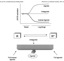
The action of a CB1 ligand at the CB1 receptor depends on whether it is an agonist,

antagonist, or inverse-agonist. These three terms are all relative to the unperturbed equilibrium

of active (R*) and inactive (R) states of the CB1 receptor. That is to say, the CB1 receptor

produces signal transduction in the absence of a ligand. It has basal activity. This activity is

referred to as constitutive activity. This is explained using a hypothetical thermodynamic

process.66 If binding of a ligand pushes the equilibrium in the direction of the active

confirmation (R*), it is considered to be an agonist. If it causes the equilibrium to favor the

inactive confirmation (R), it is considered to be an inverse agonist. If the ligand competitively

binds but shows no efficacy, that is, it stabilizes both the active and inactive confirmations in a

(12)

8

system shared by all GPCRs is considered useful but rudimentary.67-69 It provides a template for

understanding why inverse agonists produce the reverse effect of agonists (they reduce signal

transduction) and why neutral antagonists are sought (they would inhibit both agonists and

inverse agonists while not reducing basal signal transduction). CB1 receptors follow the same

receptor-ligand interactions as other GPCR. The basic equation used to quantify their

interactions is:

·

where Ki is the value at which 50% of the receptor sites are binded to by a ligand. and are

the unbound protein and ligand concentrations respectively. Though the kinetics of are the

same as for agonist, inverse agonist, and antagonist as far as setting the 50% occupancy as Ki,

may represent an agonist-receptor complex, inverse agonist-receptor complex, or antagonist-receptor complex, in binding scheme.

(13)

9

Figure 1.1.1:70_{An illustration of the dynamic between inverse agonist, antagonist, and agonist with active (R*) and inactive (R) CB} 1 receptor

confirmations is presented.

Though the CB1 receptor does express signaling without ligand binding, there are two known

lipid like ligands (agonist) that are endogenously produced. These are called the

endocannabinoids. The two endocannabinoids to have been discovered are anandamide and

2-arachidonoyl glycerol (2-AG).71-73 In in-vivo assays used to characterize the form of activity a

ligand produces, agonist of the CB1 receptor induce analgesia, catalepsia, hypomotility, and

hypothermia (in rats).74 Antagonist blockade the action of agonist. And inverse-agonist produce

effects opposite of those produce by agonist. In in-vitro assays commonly cAMP quantification

is used based on the cannabinoid receptors negative coupling to adenylyl cyclase. A decrease in

cAMP production is measurable with the administration of a CB1 agonist. [35S]-GTPγS, due to a

dual-coupling effect for the CB1 receptor, can also be used as an assay as it shares the

commonality with the CB1 as among all GPCRs in that it binds to a GTP molecule when

activated by an agonist. So an agonist will increase the binding to [35S]-GTPγS, a radiolabelled

(14)

10

neutral antagonist, and inverse agonist. Based on these two assays rimonabant is considered to

be a mild inverse agonist.76,77

Though the CB1 receptor has not been crystalized and no definite x-ray structure

obtained, the potential binding site of CB1 agonist/inverse agonist has been explored

computationally and experimentally by the use of homology and mutagenic studies. 3D

homology models are frequently based on bovine rhodopsin, a GPCR, which has been

structurally determined by x-ray crystallography at 2.8 Å resolution. And the resulting

predictions are tested by mutating specific amino acids in the presumed binding pocket to

determine if binding has increased or decreased by the aforementioned bioassays.23,78,79 From

these studies, specific amino acid residues have been identified as being directly involved in the

binding of antagonist and inverse agonist to specific binding regions of the CB1 receptor.

The CB1 receptor consists of seven hydrophobic alpha helix transmembrane segments

(TMH), an intracellular C terminus, and a 116 residue long extracellular N terminus tail, which

seems to have no relevance in receptor recognition.80 It consists of 472 total residues.70,81 There

is evidence that not all CB1 ligands bind to the same receptor site. Aminoalkylindoles, such as

WIN 55,212-2, have been shown not to bind to the same location of the receptor as anandamide

or classical cannabinoids (THC analogues), but bind to the same region as rimonabant. This has

been confirmed by mutation studies.17,18,82 This also points to the potential of there being

multiple activation confirmations. The binding site that has received the most attention is that of

(15)

11

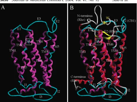
Figure 1.1.2:78_{A modeling based CB}

1 receptor to the left (A) and the crystal structure determined rhodopsin (red) superimposed with the

modeling based CB1 receptor on the right (B) are shown with the ligand binding region boxed in.

Several key areas of the receptor have been explored with modeling and mutation studies.

K3.28 (Lys192) located in the third transmembrane domain (TMH3) of the human CB1 receptor

(hCB1) was shown to be key in the inverse agonist action of rimonabant in mutation studies by

substitution with K3.28A, the non-polar residue alanine.83 This was verified when molecular

modeling techniques showed that the Lys192 residue interacts directly via hydrogen bonding

with the C3 substituent (carbonyl group) of rimonabant. This substitution does not stop

rimonabant from binding to the mutant receptor as it will still antagonize WIN 55,212-2, but

instead prevents it from acting as an inverse agonist/antagonist.84 When hydrogen bonding

(16)

12

D6.58 (Asp366) is stabilized.78 This stabilization of the Lys192-Asp366 salt bridge is thought to

be responsible for inverse agonism/antagonism as it has been shown by modeling mutagenic

studies to contribute to stabilizing the inactive state of the receptor (R).18 Studies of the binding

domain at the CB1 receptor revealed that rimonabant binds within the TMH3-4-5-6 aromatic

microdomain by aromatic stacking interactions with the F3.36 (Phe200), W6.48 (Try356),

W5.43 (Try279), and the dichlorophenyl ring system of Rimonabant, and W4.64 (Trp255),

Y5.39 (Tyr275), F5.42 (Phe278), and the monochlorophenyl ring system of Rimonabant. Also,

hydrophobic interactions occur between the piperidinyl moiety, V3.32 (Val196), F2.57 (Phe170),

Leu387, and Met384.18,78,85 These studies also reconfirmed the Lys192 hydrogen bonding

interactions with rimonabant. WIN 55, 212-2 was shown to bind in the same domain but with

aromatic stacking occurring with the Phe200, Try279, and Try356 residues. It does not stabilize

the Lys192-Asp366 salt bridge. This causes it to acts as an agonist as it stabilizes the active

confirmation. Within this domain only the F3.25A (alanine) mutation had an effect on

anandamide (which binds in the TMH2-3-6-7 region) binding, illustrating a separate binding

location for anandamide from rimonabant.18

From these binding cues, rational drug designers can begin to make sense of binding

affinity and efficacy data, and attempt to design drugs that mimic specific effects of a set of

ligands based on their structure. After key binding positions based on hydrogen bonding, sterics,

electrostatics, and aromatic stacking (other properties may also be included) have been

identified, a pharmacophore may be developed to represent a particular class of compounds, i.e.

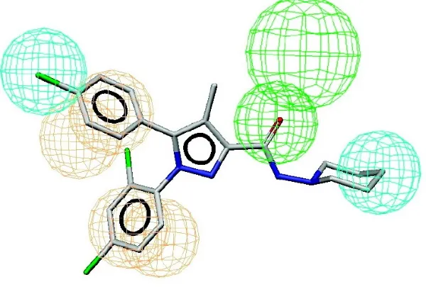
rimonabant-like inverse agonist. Figures 1.1.386 and 1.1.485 are a basic illustration of a

rimonabant-like inverse agonist pharmacophore (above), compared to rimonabant, and its

(17)

13

Figure 1.1.3:86_{A 3D pharmacophore mapped onto rimonabant: A) Cyan spheres represent hydrophobic features. B) Beige sphere represent}

(18)

14

Figure 1.1.4:85_{2D representations of the general pharmacophore’s (a) and rimonabant’s (b) interaction points with individual residues of the}

modeled CB1 receptor.

The CB1 ligands in this study are rimonabant-like compounds and follow this basic

pharmacophore model. However they are triazole-centered, as opposed to pyrazole-centered

compounds. They have been analyzed using high resolution x-ray crystallographic data,

providing a more detailed look at their surface electrostatics (as binding is achieved by

complementary surface properties), atomic basins, and bond ellipticities in an attempt to

(19)

15

Part 2: High Resolution X-Ray Crystallography and the Electron Density Distribution

In principle, all of the physical and chemical properties of a molecule are the result of its

distribution of electrons, the electron density distribution, ρ(r), and the distribution of nuclear

charges. From a knowledge of the electron density, it should be possible to obtain data useful for

drug design such as atomic charges, molecular electrostatic potentials, and intermolecular

interaction energies.87 This information can be gained in several fashions. It can be computed

theoretically using density functional theory or by a more traditional quantum mechanical

approach (molecular orbital calculations), and empirically by direct measurement of the electron

density via diffraction. This study utilizes the direct measurement of the electron density

distribution by high resolution x-ray diffraction intensity measurements at low temperature. A

high resolution description of the ED is necessary for an accurate determination of electrostatic

moments as the features in the ED responsible for the above molecular properties occur due to

slight alterations in the ED, caused by chemical bonding, at subatomic resolutions.87

In crystallography resolution can be quantified in terms of inverse angstroms (Å-1) as

2sin(θ)/λ where λ is the wavelength of the x-ray radiation (0.71073 Å from a Molybdenum

source, as used in this experimental setup) and θ is half the angle at which the x-rays diffract

relative to the incident beam. This formalism can be derived from the basic Bragg diffraction

equation

.

88_{High resolution data is collected out to approximately 1.0 Å}-1_or

greater. The use of this data not only allows for a better determination of positional and thermal

displacement parameters associated with individual atoms in the molecule, but also yields a

better deconvolution of the static electron density from the positional and thermal parameters.89

(20)

16

scattering factors, but on aspherical scattering factors. This is what makes high resolution x-ray

crystallography special in regards to a more accurate determination of the ED. What follows is a

basic description of this technique.87

The most fundamental equation in crystallography is:

ρr 1

!·" _{Equation 2.1}

where ρ(r) is the electron distribution within the unit cell,

# is the reciprocatal volume of the unit

cell, is the structure factor, H is the scattering vector (in terms of h,k,l), r is the position vector

in fractional coordinates (x,y,z) of the unit cell, and the !·" are terms of the Fourier series

expansion. The volume of the unit cell can be determined by geometric analysis and will not be

discussed here. The determination of , where the differences in the conventional independent

atom model (IAM) and high resolution x-ray crystallography are present, is more complicated.

The structure factor, a complex variable, is mathematically represented by this equation:

$%&'%&!·" (

%)

Equation 2.2

where _'_%_& is the temperature factor of atom (j), a dynamic parameter, and _$_%_& , a static

parameter, is the scattering power of atom (j) at position (r) within the unit cell and in the

direction of H, the scattering vector. Both of these variables decrease with an increase in

sin(θ)/λ.88 For anisotropic-harmonic temperature factors, the expression is as follows:

'%& !*"+·,·"

where U is the mean-square displacement amplitude matrix. This equation is the result of the

Fourier transform of the probability distribution function (pdf or P(u)) as a function of the

(21)

17

vibration about the equilibrium position of atom (j) which follows a normal distribution. Higher

order treatments of thermal motion (anisotropic-anharmonic motion) may be treated with the

Gram-Charlier expansion.90 The expression for aspherical scattering is:

$%& - ρ%.!·"/. Equation 2.3

where ρ_%. is the electron density of atom (j) at position (r). ρ_%. is represented using the

Hansen-Coppens formalism91:

ρ%. ρ0. 1 2ρ23. 1 ρ34. Equation 2.4

ρ0. is the core electron density expressed as a spherical function. ρ23. is the valence shell

electron density (expressed by a spherical harmonic monopole), normalized to one electron, with

an expansion-contraction parameter k that allows the monopole to scale in size. ₂ is the

population parameter used to adjust the value of the monopole. _ρ₃4_. is an expansion of

spherical harmonic multipoles that takes into account aspherical valence shell electron

deformations due to chemical bonding. It has its own expansion-contraction parameter 34.92 Its

expression is:

ρ34r 5634 6

. 67 6

7) 6

867_.r Equation 2.5

The radial functions ₅₆_. are normalized Slater functions:

5634. 3 496:;

<= 1 2! .96 @+" Equation 2.6

867A_" are normalized spherical harmonics that are multiplied by a population parameter in

order to attenuate the amount of electron density relocated. The _ρ₃4_. do not alter the total

(22)

18

to another part of the atomic environment they describe. All of these parameters are centered

about the nucleus of the atom who’s ED they describe.91

Thermal parameters are more accurately determined using higher resolution data. This is

based on the principle that the core electrons are relatively unaffected by chemical bonding. As

a result, near the core of each atom there is a sharp peak in electron density that is relatively

unaffected by bonding as in the case of valence electrons. At high angle diffraction, or high

resolution data _B

C 0.75 Å I, the valence or bond density contribution to the Bragg

reflections is greatly reduced due to limitations of the x-ray wavelength and electron density

falling out of phase.89 Due to this phenomenon, it is approximated that all of the electron density

contributing to the high angle Bragg reflections are from each atom’s core. As core electrons

occupy space near the nucleus and as mentioned earlier are not affected by chemical bonding,

and therefore of spherical geometry, the nuclear probability distribution functions are refined

using ED modeled on spherical scattering factors including this high resolution data. In an

attempt to limit the effect that temperature has on x-ray diffraction, as higher thermal parameters

result in lower diffraction at higher angles and to ensure better signal to noise ratios at higher

angles, data sets are collected on crystals that are cooled using a cryostream of nitrogen gas. In

this experimental setup data were collected at 120 K. The result is better position and thermal

parameters due to lower temperatures increasing the angle which x-ray intensities may be

observed, and thus the inclusion of data at higher angles in the least-squares refinement.

As the actual data collected, || (observed as the intensity of reflection H), contains

information on both the static scattering factor and the dynamic temperature factor, the two must

be separated in order to obtain the static ED.93 This process is called deconvolution and relies on

(23)

19

product of the Fourier transforms of the individual functions _{KLM$ N OP LM$P · LMOPQ}.94 As

the dynamic electron density of an atom is a convolution of static electron density with the

probability density function [_ρ_%. ρ_%._RSTS0 _{N U}] and the scattering factor is the Fourier

transform of the static electron density _$_{%& V ρ%}_.!·"_/.or$_%& LWρ_%.X and

the temperature factor is the Fourier transform of the probability distribution, '_%&

V U!·"_du_or_'

%& LMUP, then the Fourier transform of the convolution of

ρ%.RSTS0 with Uis the dynamic scattering factor which includes both the static aspherical

scattering factor and the temperature factors. That is:

LWρ%. N UX LWρ%.X · LMUP = $%& · '%& Equation 2.7

Once refined and deconvoluted the thermal parameters are subjected to a Hirshfeld test95_to

ensure their reasonability. In the Hirshfeld test, the mean square amplitudes of displacement due

to thermal motion for bonded atoms are compared along the bond direction.

Accurate determination of _'_%_& from refinement of high resolution data at low

temperature and $_%& with the use of the Hansen-Coppens formalism for asymmetric scattering

factors, which introduces more refinable parameters, ultimately leads to a better model of the

ED.91 The model parameters are refined using a least-squares method where the difference

between observed and calculated structure factors is minimized by setting the derivative of the

difference equal to 0,

0 YM|Z| [ 3|0|P\|3_]^0|

% Equation 2.8

where |_Z| and |₀| are the magnitudes of the observed and calculated structure factors

(24)

20

scale as the calculated structure factors. The validity of the model may be tested by computing

an R-factor which is the fraction of disagreement between |_Z| and |₀| in terms of |_Z|,

5 _∑a|_∑|Z| [ |0|a

Z| b Equation 2.9

Major improvements are noticed in this value after refinement with aspherical scattering factors

compared to independent atom model (IAM), a rudimentary refinement in which scattering

factors are approximated by spherical functions.93 It can also be visualized in order to assess the

fit of the aspherical scattering factors to individual atoms or group of atoms using a Fourier

difference map. This is called the residual density.

∆ρ"dR e1_{fg |}Z| [ |0|

hi !·" Equation 2.10

Since the phase factor j cannot be measured experimentally, both the observed and calculated

structure factors use the calculated phase information. This is referred to as the model biasing

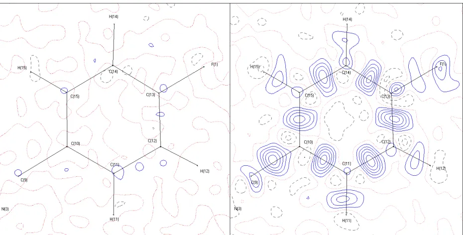
problem as the model is biased towards the calculated phases.88 In Figure 1.2.1 the

improvements to the fit of the model for one of the aromatic rings in the compound AVG-229Ph

can be seen due to the employment of aspherical scattering factors and high resolution x-ray

(25)

21

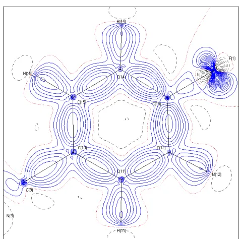
Figure 1.2.1: An illustration of the difference density with spherical scattering factors (right) and aspherical scattering factors (left). The lower R-factor and lower peaks in the residual density map indicate a substantial improvement in the aspherical model compared to the spherical IAM model for the ED. Contours are in 0.1 · Å ;_{increments. Blue solid lines are positive increments. Grey dashed lines are negative. Dotted red}

lines hold a value of zero. To the left is a residual map in the plane of C(10), C(12), and C(14), part of a ring system in AVG-229Ph, at an approximate resolution of sin(θ)/λ = 1.1 Å . The final refinement on F of the complete structure is R1 = 0.0248. To the right is the same ring

system refined with spherical scattering factors. The final refinement on F of the complete structure is R1 = 0.0462.

When a difference density is calculated by subtracting the density corresponding to

neutral spherical atoms from the electron density of the crystal, is is called an electron

deformation density (EDD), because it reveals how atoms are deformed due to chemical bonding

and their crystal environment.

∆ρ(r)EDD = ρ(r)multi - ρ(r)promolecule Equation 2.11

If _ρ_%._0"kRST6 is calculated by Fourier transformation of the experimental structure factors, _Z,

the deformation density is called an ‘experimental dynamic deformation density’ (as seen in the

right side of Figure 1.2.1). This density will include the smearing due to thermal motion of the

atoms, and will suffer from noise due to errors in the x-ray intensity measurements and series

termination errors due to the finite resolution of the experiment.

If, however, _ρ_%._0"kRST6 is calculated by direct evaluation of the multipole functions

(26)

22

is called the ‘model electron deformation density’, and can be either a ‘dynamic’ density if the

thermal motion is included, or a ‘static’ density if the thermal motion is omitted from the

calculation.96,97 Below is the (static) deformation density of the same ring system as in Figure

1.2.2.

Figure 1.2.2: Deformation density map of the same ring system in displayed in Figure 1.2.1. Contours are in 0.1 · Å ;_{increments. Blue solid}

lines are positive increments. Grey dashed lines are negative. Dotted red lines hold a value of zero.

It is clear that electron density has moved into regions between atoms to create chemical bonds.

This density may be analyzed to determine any one electron property such as atomic charge,

bond order, and aromatic bonding character (ellipticity). Once all qualifying measures of the

model’s fit to the data have been checked and reviewed for error and “chemical sense” (if the

results seem chemically reasonable), the molecular properties and moments of interest that are

(27)

23

Part 3: Useful Molecular Properties Determined From the Electron Density Distribution

For drug design, the principle molecular properties of interest include the electrostatic

potential, _., net atomic charges, _lm, and magnitude and ellipticity of the density in the

bonding region between atoms.98 π-stacking is considered to be a major interaction with the CB1

receptor binding site of the ligands tested. Each property of an individual molecule is derived

from the total electronic distribution and quantitatively analyzed relative to the rest of the

molecule set in an attempt to correlate molecular features with pharmacological affinity in (Ki).

Atomic charges are calculated by integrating the atomic basins of each nuclei in accord with

Bader’s quantum theory of atoms in molecules (QTAIM).99

A. Atomic Charges and QTAIM

The assignment of net charges has a long history in chemistry, and has proven to be a

useful method of prediction of electrostatic interactions between molecules. Atomic charge is

also an indicator of an atom’s capacity for hydrogen bonding. For instance if an oxygen or

nitrogen is highly negative, it may act as a hydrogen bond acceptor. If in the right orientation,

hydrogen bonds will contribute to the stabilizing of the ligand-receptor complex. In addition to

molecular shape, a complimentary distribution of atomic charges may stabilize the complex

through electrostatic interactions.100 This gain in stability may also be true of other

supramolecular interactions that rely on similar mechanisms. For this reason atomic charges are

tabulated and analyzed. In order to compute the atomic charges of an atom in a molecule, one

must partition the molecular density among the atoms of the molecule. In most schemes for

(28)

24

In QTAIM, defining where one atom ends and where another begins in a molecule is not

arbitrary. In order to properly understand the concept of an atom in a molecule, we must first

provide a basic background on QTAIM topological analysis of the electron density. This is not a

comprehensive review of the topic and is only intended to provide a meaningful understanding of

atomic basins and their charges.

Most attempts to obtain atomic charges and understand chemical bonding have been

based on molecular wavefunctions which are solutions to Schrödinger’s equation.99 Although

widely used, these methods are highly dependent on the approximations used, such as basis set

size, and suffer from the arbitrary nature of the partitioning method. Schrödinger himself warned

against attaching physical significance to wavefunctions.101 However, the properties of

chemistry and physics are based on phenomenon in real space. QTAIM was developed as a real

space description of the charge density distributions. Its topological features serve as the carrier

of physical information regarding the concepts of atoms, bonds, structure, and structural stability.

Topological features of _n. are associated with “critical points” (cp’s), locations in the

electron density where the first derivative of n. is equal to zero (on.₀ 0. They are

defined by the behavior of the ED surrounding them. The second derivative matrix, the Hessian

matrix, of _n. determines whether a cp is of a topology of (3,-3) [local maximum at _.₀ typically

at a nuclear attractor], (3,-1) [local maximum at _.₀ in the plane defined by two axes and a

minimum in the third, typically at the center of a bond], (3,+1) [local minimum at .₀ in two axes

and a maximum in the third, typically occurs at the interior of a ring system], or (3,+3) [ local

minimum at _.₀ typically at the interior of a cage system]. When taking the gradient field vector

(gradient path) starting from an arbitrary point and stepwise progressing to on.₀ 0, all paths

(29)

25

attractors to ED, which makes sense. A ridge line of density connects bonded atoms, with a

(3,-1) cp at the minimum (saddle point) along the ridge. Topologically an interatomic surface can be

defined as the set of trajectories that terminate at a (3,-1) cp. This results in a partitioning of the

ED in a molecule into individual point attractors centered at “atoms in the molecule” and the

surrounding “atomic basin”. Where one atomic partition ends and the other begins is considered

an interatomic surface (_p_qr) of each respective domain. It can be very elegantly expressed as:

on. · s. 0 for each point on the surface S(r) Equation 3.1

where _s. is the unit vector normal to the surface being evaluated at r. This is called the

zero-flux surface and it defines the atomic basin, and contains the nucleus and volume of the electron

density associated with it. From this definition of an atom in a molecule, the atomic charge can

be determined by taking the integral of the difference between the nuclear and electronic charges

over the atomic basin within the zero-flux surface.

lm tu[ vm Equation 3.2

tu is the electronic charge and vm is the nuclear charge. The result is a definition of atomic

charge and atomic volume based only on the electron density distribution which is independent

of the basis set, or the method used for obtaining the density. Below is a graph of the path

trajectories in the plane of ring system from Part: 2 of this intro to illustrate in 2D how these

(30)

26

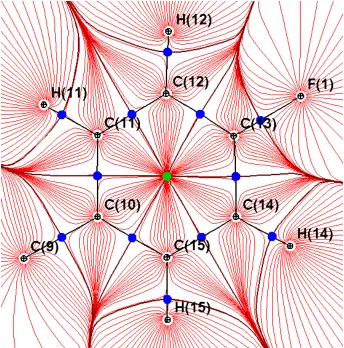
Figure 1.3.1: A 2D plane of trajectory paths in red through a ring system in AVG-229Ph. The blue dots are saddle points (3,-1). And the green dot is a ring center point (3,+1). Straight black lines represent chemical bonds. Curved black lines show the surface of the atomic basin as it passes though the plane.

B. The Electrostatic Potential and Binding

The electrostatic potential (ESP) is considered to be a molecular property which is highly

predictive of noncovalent interactions. This includes hydrogen bonding and interactions that

occur at the “surface” of a molecule and thus is expected to play a major role in initial phases of

ligand recognition by a receptor site.102_{Therefore we consider the computation of the ESP at the}

molecular surface of these compounds to hold useful information about the activity of each

molecule. This is because a ligand’s surface will be attracted to its negative compliment within

the receptor site causing it to approach and begin to orient. Along with complementary surface

(31)

27

neutral the ESP is at a molecule’s surface, the less polar it may appear to surrounding

molecules.103 This is far from the only factor involved in ligand-receptor binding. It does not

include entropy factors such as changes in the degrees of freedom of both the ligand or of the

surrounding environment. It also does not account directly for changes in molecular

conformation as the molecules are not rigid. But it is necessary at the outset of ligand

recognition.104

Before calculating the ESP, the value of an isodensity surface must be determined. This

is done by calculation of the ED at a particular isodensity value. It should also be taken into

consideration the effects that a perturbing field, such as that induced by an approaching

molecule, will have on the ESP at that density level. The nearer the ESP is to the “inside” of a

molecule, the greater the density and the less effected it is by outside forces. The isodensity

value commonly used as a molecular envelope in the experimental determination of ESP is 0.007

· Å ;_{(approximately 0.001 au in e/bohr}3_{) as proposed separately by Bader, and Politzer and}

Murray.100,105 Other low values are valid. At this isodensity surface, features such as the lone

pairs and π electronic charge are still apparent. Below is a visualization of a typical isodensity

(32)

28

Figure 1.3.2: An example of an isodensity surface of AVG-229Ph at the value of 0.007 · Å ;_.

If one has both the electron distribution and the charge and location of the nuclei in the

molecule, calculating the ESP is relatively straight forward. The ESP is calculated as:

. _|5tq

q[ .| [

-n.4_/.4

|.4_{[ .|} Equation 3.3

tq is the atomic charge of atom A at the position of 5q. |5q[ .| is the distance from the nuclei

to point r, which will be calculated on the isodensity surface. And the integral is the electronic

charge produced by the ED at a distance of |.4[ .| to point .4. The total integral of the ED is a

positive value and is then subtracted from the sum of the effects of all _t_q to account for the

negative charge of the electron.100 The data on which the ESP is based are obtained in the

crystalline environment, and the forces between the individual molecules in the crystal are

electrostatic and therefore are complimentary to each other. Thus, this ESP calculation may be

(33)

29

wavefunctions for a molecule in a vacuum.104 The ESP is not to be calculated at every point, but

only at points where _{n. 0.007 · Å} ;. The resulting ESP is the surface electrostatic

potential and is denoted as _R.106_{When projected with a color gradient it may be analyzed}

visually to determine whether it is positive or negative as well as the strength of the potential. In

this fashion one may compare multiple molecules against one another and compare the ESP with

other data such as each molecule’s affinity, to identify any regions whose ESP may play an

important role in binding. Figure 1.3.3 shows the ESP projected on to the molecular surface

from Figure 1.3.2. A similar type of analysis has been performed previously by Politzer and

Murray on a series of compounds to assess the toxicity of ligands (dibenzo-p-dioxins) that bind

to a porphine like receptor, the cytosolic receptor. It was found in that study, and later verified

by modeling studies, that two compounds exhibited very different toxicities due to an

accumulation of or lack of negative ESP in the center ring system. This feature of negative ESP

in dibenzo-p-dioxin, centered around oxygen groups, prevented it from binding due to

interactions with nitrogen lone pairs within the receptor site. The added chloro-groups in

2,3,7,8-tetrachlorodibenso-p-dioxin, which is structurally similar otherwise, provided enough

electronegativity to prevent this accumulation of negative ESP on the oxygen groups of the

molecule. This change in ESP (observed in other compounds as well) increased binding to the

receptor causing greater toxicity. Other compounds similar in structure with the added

chloro-groups that were able to maintain the negative ESP showed reduced toxicity as well.100 Efforts

to experimentally determine the affinity of compounds from experimental electron distributions

(34)

30

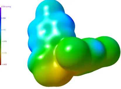
Figure 1.3.3: The isodensity surface from Figure 1.3.2 with the ESP mapped on to the molecular envelope.

Though very local alterations in the ESP may change binding affinity, it is also

recognized that more global parameters may be predictive of binding as well.100 This is because

not all ligand-receptor binding occurs in the same fashion. Some ligands-receptor interactions

are due to broader contacts. To asses this, it is possible to calculate several globally defined

statistics of the ESP to analyze the general interaction properties functions (GIPF). These are

properties introduced by Politzer and Murray.107,108 Of interest are the average deviation (w),

total variance(x_yzy), balance parameter (f), and maximum and minimum values of the ESP.

w 1_{< |}R{ [ |R| 9

)

Equation 3.4

xyzy x:1 x _{j }}1 R:K{%Q [ |R:~ h

%)

1_}1 R K{%Q [ |R ~

@)

(35)

31

f _xj:x

SZS Equation 3.6

C. Bond Ellipticity as an Indicator of Aromaticity

Another property of the ED of interest is the bond ellipticity, as π-stacking is considered

to be a significant factor in the binding of CB1 ligands. x-bonds are cylindrically symmetric

while π-bonds are elongated perpendicular to the molecular plane. For single or double bonds,

the amount of π character a bond has can be quantified by its ellipticity. Single bonds display an

ellipticity of close to zero while double bonds are near 0.2 among C-C interactions.109 In

QTAIM, bond ellipticity is calculated as:

[ 1 Equation 3.7

where and are the principle curvatures perpendicular to the bond path (the two negative

eigenvalues of the Hessian matrix). is the component that undergoes contraction (thus _<

). It will be analyzed to see if molecules with higher ellipticity in their aromatic ring systems

(36)

32

Methods

Part 1: Crystallization

Each crystal in this study was obtained by slow solvent evaporation from a solution

contained in a scintillation vial. By covering the vial with parafilm with small needle sized holes

poked in it, solvent was allowed to slowly evaporate at ambient temperature and pressure. Many

different solvents and mixed solvents with varying ratios of solvents were used until adequate

resulting crystals were grown. Frequently crystals took several weeks or months to form, if at

all, as the compounds are prone to retain non-polar solvents. Non-polar solvents generated the

best results. Compounds rarely dissolved in polar solvents. And attempts to “crash” crystals out

of solution via polar solvent dilution or by increasing the temperature to increase solubility, then

reducing the temperature to bring the saturated solution beyond its saturation point, resulted in

unsuitable crystals due to small size or disorder within the crystal on a molecular level.

Diffusion methods were also explored but generally failed to generate usable crystals within the

time invested. After evaporation of solvent, the vials were examined under a stereoscopic

microscope with light polarizing capabilities to determine if potential crystalline samples had

formed. Only crystals that appeared under polarized light to be single, non-twinned crystals

without satellite crystals were considered as candidates for data collection. If crystals were too

large in any dimension to remain within the diameter of the x-ray beam during the experiment, a

razor blade was used alter their shape. This was frequently problematic as many compounds

formed brittle crystals that shattered under the pressure of the blade. Table 1 contains details on

solvents used to obtain the crystals used for successful data collection, and the morphology of

(37)

33

Compound Mol. Formula Solvent Crystal Dimensions (in mm) Morphology

AVG-229Ph C21 N2 O2 Cl2 F1 H13 DCM 0.4 x 0.5 x 0.5 Block

HS-P183 C17 N3 O2 Cl3 H12 1 THF : 1 EtOH 0.15 X 0.3 X 0.5 Plate

HS-P226 C17 N3 O2 Cl3 H12 THF 0.5 X 0.5 X 0.6 Block

HS-P53-1 C16 N3 O2 Cl2 H11 1 THF : 2 EtOH 0.17 x 0.2 x 0.4 Needle

HS-P53-2 C14 N1 Cl2 H9

1 THF : 1 EtOH : 1 CHCl3

0.1 x 0.5 x 0.5

Plate

HS-P57-2 C14 N3 Cl3 H8 CHCl3 0.25 x 0.5 x 0.6 Plate

HS-P57-3 C17 N3 O2 Cl3 H12 1 THF : 1 Acetone 0.2 x 0.5 x 0.5 Plate

HS-P57-4 C18 N3 O2 Cl3 H14 EtOH 0.25 x 0.5 x 0.5 Plate

HS-P57-7 C21 N3 O2 Cl3 H18 1 THF : 3 Acetone 0.07 x 0.2 x 0.5 Needle

HS-P69 C20 N5 O1 Cl3 H18 1 DCM : 3EtOAc 0.15 x 0.25 x 0.5 Plate

Table 2.1.1: Basic compound and crystal information.

Part 2: Crystal Mounting and Data Collection

Once crystals were grown, selected, and trimmed, they were glued to a glass needle under

the microscope with an amorphous epoxy resin. Each needle was then individually placed at the

end of a goniometer head and fitted on to the goniometer of the x-ray diffractometer. Each

crystal was centered in the x-ray beam path and the cooling nozzle lowered into place. After

mounting, cooling to the final temperature, and centering the crystal, collecting data was begun.

Data were collected on a Bruker Kappa Apex II 4-circle diffractometer with each sample

cooled to 120(2) K via a gaseous N2 stream generated by an Oxford Cryostream 700 low

temperature device. A Molybdenum target x-ray source and graphite monochromator was used

producing x-rays with a wavelength of 0.71073 Å.110 An Apex II CCD detector was placed

40.00 mm or 60.00 mm away from the sample, depending on the size of the unit cell.

Compounds with larger unit cell dimensions were collected at 60.00 mm to avoid reflection

overlap as larger direct space cell dimensions result in contracted reciprocal space cell

dimensions, the space data is collected in. The length of x-ray exposure per frame varied from

20 to 300 seconds depending on the 2θ angle range being observed (higher angles require longer

(38)

34

was defined by a 0.6 mm collimator which limited the size of the uniform region of the x-ray

beam, and thus the size of the crystal sample that could be used. Scans were conducted varying

either omega or phi angles with the other axes remaining fixed per scan. That is, for an omega

scan over 115 degrees, phi, chi, and 2θ angles were set at fixed values while omega was varied.

Each frame was collected over a 0.5 degree sweep for the 20 to 300 seconds allotted for that

collection. The number of reflections, redundancy, and peak resolution differed from compound

to compound. The consistency/internal agreement of the data was verified against itself and

quantified in R(int):88

R |[ |

Equation 2.2

Table 2.2.2 is a basic description of each data set after data processing.

Compound Unique Reflections Avg. Redundancy Peak Resolution (Å) R(int) x 100

AVG-229Ph 15,821 12.86 0.48 1.83

HS-P183 18,220 6.37 0.45 2.28

HS-P226 14,985 7.17 0.456 1.51

HS-P53-1 11,923 8.74 0.5 2.41

HS-P53-2 9,174 9.71 0.47 2.47

HS-P57-2 10,494 8.24 0.47 2.24

HS-P57-3 12,952 4.4 0.47 1.53

HS-P57-4 42,192 15.7 0.55 2.53

HS-P57-7 10,740 7.51 0.45 2.39

HS-P69 15,848 9.43 0.52 2.00

Table 2.2.2: An overview of crystal data quality.

Part 3: Independent Atom Model Refinement Using Apex2/Shelx

After data were collected for a crystal, they were was processed and refined using the

Apex2/Shelx software package.111,112_{Initially, a small set of reflections were indexed and used}

to determine the unit cell of each compound, and the Bravais lattice was determined using

geometric analysis. This unit cell was then used to predict the locations of all reflections to be

integrated for total intensity. The integration program “searches” for a reflection in the predicted

(39)

35

entire reflection and subtracts out the background noise by measuring the intensity surrounding

each reflection. Reflections typically span several frames and it is the total intensity count across

these frames that yield the integrated intensity value. Also, using lower angle date, where the

signal to noise ratio is higher, a reflection’s 3D profile is computed to help box size optimization

and noise subtraction of weaker reflections and reflections that occur at greater 2θ values. This

is done because the signal to noise ratio at higher angles or higher resolution is much lower.

During this process, cell dimensions are further refined using a larger set of reflections. Once

reflection intensities have been determined, the data are corrected for absorption in the

subroutine Scale, formerly known as SADABS.113 This corrects for absorption of x-rays that

have to pass through a greater or lesser distance through the crystal, as the crystals are not

spherical. This is done by comparing differences in multiple measurements of the intensities that

should be equivalent due to Friedel’s Law or symmetry.114,115 The shape of the crystal’s

absorption correction surface is defined by refining coefficients of a spherical harmonic

expansion, which is used to calculate corrections for the remaining reflections. From this, each

reflection’s intensity is adjusted for absorption. The corrected file of intensities is analyzed

using Xprep.112 Xprep determines the space group of a crystal by looking for systematic absences

or “holes” in an x-ray pattern that are caused by the presence of specific symmetry elements.

Along with the Bravais lattice, this information is used to assign a space group may. Xprep

outputs an intensity data file (.hkl) for Shelx which is used to refine the parameters based on the

independent atom model (IAM).96,111. Also, for future use in the refinement strategy, a merged

HKL file is generated for use by the program XD2006116 in which all duplicate data is averaged

with the data spread present as a standard deviation for each observation. Structure solution was

(40)

36

the best figure of merit was used to calculate an approximate electron density (e-map). The XP

module with Shelx was used to assign atoms to peaks in the electron density, referred to as

Q-peaks, which also assigns the spherical scattering factor associated with that atom in the position

of the Q-peak. These are tabulated within Shelx. XP produces an instructions file (.ins). This

file, with its new scattering factors, in turn was used to refine thermal parameters and atomic

positions via least squares with the XL module. XL produces a results file (.res) that was used

by XP for further manipulation of atom assignment. This process of refining positional and

thermal parameters with least squares in XL (which also generates new Q-peaks) and assigning

atoms was performed repeatedly until no further improvements could be made. On all occasions

for the final data sets used in the study, after adding anisotropic thermal parameters, and peaks

corresponding to hydrogen atoms were clearly present in the difference map generated by XL,

and hydrogen atoms were added to the least squares refinement model. All final data sets were

absent of disorder and had reasonable thermal parameters, a prerequisite for high resolution

analysis of the ED. Once satisfactory results were achieved at this stage, the resulting .ins file

and merged .hkl file were exported to XD2006 for further refinement.116 Varying R-factors were

recorded for each compound and are tabulated in the results section.

Part 4: XD2006 and the Hansen-Coppens Formalism with Aspherical Scattering Factors

The computer program XD2006 was used for the refinement of high resolution data with

aspherical scattering factors using the Hansen-Coppens multipole formalism.91,116 The Windows

interface for XD2006 is shown in Figure 2.4.1 where graphics are displayed and text

notifications of refinements in process appear. In this case a simple stick model of AVG-229Ph

(41)

37

Figure 2.4.1: XD2006 interface screen.

Once a refinement has been completed in APEX2112_{and the instructions and HKL files copied to}

a working directory in the XD2006 file system, the XDINI module is executed. This produces

files usable to XD2006, namely the input file (.inp), a XD2006 compatible HKL file, and a

master file (.mas). The input file is where the parameters (temperature parameters, positions,

multipoles, kappa values) of the molecule are written. This file is ultimately the description of

the electron density of the asymmetric unit and is used to calculate all properties derived from it

(42)

38

and standard deviations of each reflection. The master file contains all basic information about

the cell (dimensions, symmetry operations, etc.) and instructions for each individual module.

The primary modules of XD2006 involved in this study are XDLSM, XDFOUR, XDPROP and

TOPXD. To illustrate how a refinement is performed in XD2006 and how these modules are

utilized, the refinement of AVG-229Ph will be detailed. All other compounds are refined in the

same basic fashion.

After usable files for XD2006 have been created, a local coordinate system must be

assigned to each atom in the asymmetric unit. This must be done keeping in mind the shape of

spherical harmonic functions that will be used to refine the ED and their orientation to each axis.

Shown below is a segment of the XDLSM module portion of the master file which contains a list

of atoms in the first column (ATOM) that corresponds to the molecule in the graphical display

above. This is the atom for which the local coordinate system will be centered. In the second

column (ATOM0) is the atom whose position will serve as the direction of a vector for which an

axis will be assigned. This axis assignment is in the third column (AX1). The fourth (ATOM1),

fifth (ATOM2), and sixth (AX2) columns function in the same fashion except that the only the

components perpendicular to the previous vector are used. This resulting vector is also centered

at the atom in the first column. The third axis (the only unlabeled axis left) is generated normal

to the plane defined by the first two vectors. The seventh column (R/L) defines the handedness

of the axis system and therefore the direction of the remaining axis. This means that for local

coordinates of O(2), the vector from O(2) to C(7) is defined as the x-axis. The component of the

vector from C(8) to O(1) that is perpendicular to the previous axis is defined as the y-axis. And

the normal vector to the resulting plane is the z-axis in the direction that creates a right handed

(43)

39

Figure 2.4.2: Atom list, local coordinate setup, chemical constraint, and refinement options layout of an XD2006 master file.

Also present in this section is the level of treatment for thermal parameters designated in column

(44)

40

anisotropic harmonic thermal parameters, and 3 and 4 designate anisotropic-anharmonic thermal

parameters. In most cases anisotropic-harmonic thermal parameters are sufficient. But in this

model Cl(1) refined better with anharmonic anisotropic thermal parameters.117,118 This was

evident in an improvement in the residual map of both atoms. Column 9 (TBL) defines which

core and valence scattering factor tables are used for each atom. Column 10 (KAP) specifies

which set of kappa values will be refined with that particular atom. Several atoms that are of a

similar environment will usually use the same kappa set. When XDLSM performs a least

squares refinement on a set of kappas it considers all atoms associated with that set. Column 11

(LMX) designates the level of the spherical harmonic multipoles whose populations may be

refined for that atom.91 Designations of these spherical harmonics are as follows: 0–monopole,

1–dipole, 2–quadrapole, 3–octapole, and 4–hexadecapole. If 2 is selected as in the case of the

hydrogen atoms monopole, dipole, and quadrapole spherical harmonic functions may be used to

refine the atoms ED but not octapole and hexadecapole functions. All other atoms in this study

that are not hydrogen use up to the hexadecapolar level of refinement. Column 12 (SITESYM)

was not used for any compounds as no atoms were located on special symmetry sites. The last

column (CHEMCON) is used to apply chemical constraints to the multipole parameters of the

atom in that row to be identical to those of the labeled atom. In this case Cl(2)’s multipoles are

constrained to be the same as Cl(1)’s. The least-squares process is modified so that the resulting

parameters are those that provide the best overall fit at both atoms.119 Typically all aliphatic

hydrogens are constrained to be equal as well as all aromatic hydrogens. The benefit of these

constraints is that there is a reduction in the number of refined parameters. For the optimization

problem to be over determined, for every parameter to be refined there must be more than one

High Resolution X-ray Diffraction Analysis of CB1 Receptor Antagonists as a Means to Explore Binding Affinity

ScholarWorks@UNO

ScholarWorks@UNO

High Resolution X-ray Diffraction Analysis of CB1 Receptor

High Resolution X-ray Diffraction Analysis of CB1 Receptor

Antagonists as a Means to Explore Binding Affinity

Antagonists as a Means to Explore Binding Affinity

Table of Contents

Abstract

Introduction

Methods