in the population sciences published by the Max Planck Institute for Demographic Research Konrad-Zuse Str. 1, D-18057 Rostock · GERMANY www.demographic-research.org
DEMOGRAPHIC RESEARCH
VOLUME 24, ARTICLE 25, PAGES 611-632
PUBLISHED 21 APRIL 2011
http://www.demographic-research.org/Volumes/Vol24/25/ DOI: 10.4054/DemRes.2011.24.25
Research Article
On the correspondence between CAL
and lagged cohort life expectancy
Michel Guillot
Hyun Sik Kim
© 2011 Michel Guillot & Hyun Sik Kim.
This open-access work is published under the terms of the Creative Commons Attribution NonCommercial License 2.0 Germany, which permits use, reproduction & distribution in any medium for non-commercial purposes, provided the original author(s) and source are given credit.
1 Introduction 612
2 CAL and LCLE 613
2.1 CAL, the Cross-sectional Average length of Life 613
2.2 LCLE, the Lagged Cohort Life Expectancy 614
2.3 Correspondence between the two indexes 615
3 Mortality models producing an exact or near exact correspondence 616
3.1 Linear shift pattern of mortality change 616
3.2 Gompertz pattern of mortality with constant log-linear decline 618
4 Correspondence between CAL and LCLE in actual populations 620
4.1 Database 620
4.2 Measurement issues 620
4.3 Example: Swedish females 621
4.4 Generalization 624
5 Discussion 628
6 Acknowledgements 630
On the correspondence between CAL and
lagged cohort life expectancy
Michel Guillot1
Hyun Sik Kim2
Abstract
It has been established that under certain mortality assumptions, the current value of the Cross-sectional Average length of Life (CAL) is equal to the life expectancy for the cohort currently reaching its life expectancy. This correspondence is important, because the life expectancy for the cohort currently reaching its life expectancy, or lagged cohort life expectancy (LCLE), has been discussed in the tempo literature as a summary mortality measure of substantive interest. In this paper, we build on previous work by evaluating the extent to which the correspondence holds in actual populations. We also discuss the implications of the CAL-LCLE correspondence (or lack thereof) for using CAL as a measure of cohort life expectancy, and for understanding the connection between CAL, LCLE, and underlying period mortality conditions.
1 Population Studies Center, University of Pennsylvania, 3718 Locust Walk, Philadelphia PA 19104, USA.
E-mail: [email protected].
2 Center for Demography and Ecology, University of Wisconsin-Madison, 1180 Observatory Drive, Madison
1. Introduction
In recent years several alternative summary measures of mortality have emerged in the context of the debate on “tempo effects.” The existence of tempo effects in mortality is still a controversial issue. Nonetheless this debate has generated a healthy discussion about various ways of summarizing a population’s mortality experience.
One measure that has been discussed in the context of this debate is the Cross-sectional Average length of Life (CAL). CAL’s original purpose was not to address tempo effects in mortality. In fact CAL was developed prior to Bongaarts and Feeney’s proposition that there are tempo effects in mortality, and it has its own interpretation aside from tempo effects. Nonetheless CAL is closely related to Bongaarts and Feeney’s tempo-adjusted life expectancy. In particular, the two indicators are equal to one another when mortality follows some specific patterns.
One other finding that has emerged from the tempo debate is the fact that, under some assumptions, CAL is equal to the life expectancy for the cohort currently reaching its life expectancy. The life expectancy for the cohort currently reaching its life expectancy, or lagged cohort life expectancy (LCLE), is an interesting index in itself, as we will explain below. However it cannot be observed for the current year, because a cohort’s life expectancy or mean age at death cannot be observed until the cohort is extinct, i.e., many years after the time at which that mean age at death was reached. CAL, however, can be readily calculated for the current year with no reference to the future, as long as sufficient historical mortality data are available. Therefore the existence of a precise and consistent correspondence between CAL and LCLE could justify the use of CAL as a proxy for LCLE, an unobservable yet informative quantity. Another reason for further studying the CAL-LCLE correspondence is the fact that Bongaarts and Feeney see the existence of a correspondence between CAL (or their tempo-adjusted life expectancy) and LCLE as evidence in support of their proposition that current period life expectancy overestimates life expectancy under current mortality conditions.
2. CAL and LCLE
2.1 CAL, the Cross-sectional Average length of Life
CAL is defined as follows:
dx
∫
∞ − = 0 ) , ( )(t p xt x
CAL c (1)
where pc(x, t-x) is the probability of surviving from birth to age x for the cohort born at time t-x. In a population, pc(x, t-x) corresponds to the proportion of cohort survivors for the cohort aged x at time t. Simply put, CAL is the cross-sectional sum of proportions of cohort survivors at a given time. CAL is a mortality measure that summarizes the mortality history of all cohorts present in a population at a given time. It also corresponds to the size of the “birth-standardized,” or “constant-births” population, i.e., the total size of a population with a constant unit stream of births exposed to actual, changing mortality trends.
Equation (1) takes into account mortality at all ages. Like the life expectancy, CAL can also be calculated for any starting age x:
∫
∞ − − = x c c x a t x p a t a p t CAL ) , ( ) , ( )( da (2)
By involving cohort survival to age a conditional on survival to age x, CALx takes into account mortality rates above age x only.
CAL was first defined by Brouard (1986). Further developments were introduced by Guillot (1999, 2003), including equations for the relationship between CAL change and period mortality, and the population size interpretation of CAL. Guillot (2005) has also shown that the discrepancy between e0 and CAL during a given year can be interpreted in terms of population momentum. More recently Wachter (2005) has shown that CAL is essentially a weighted average of past levels of period life expectancy.
to one another (Bongaarts and Feeney 2003). Under steady mortality decline, these three indicators are all lower than period life expectancy (Bongaarts 2005).
2.2 LCLE, the Lagged Cohort Life Expectancy
Each cohort that is now extinct has a known value for its life expectancy at birth:
)dx
∫
∞
=
0 0(t) p (x,t
eC c (3)
In closed populations cohort life expectancy is equal to the observed mean age at death for that cohort. For cohorts that are not yet extinct, their remaining mortality experience is unknown, and thus their life expectancy or mean age at death is unknown. Unless some assumption about future mortality is made, cohort life expectancy can be calculated with certainty only for cohorts that are extinct or near extinct.
The year at which a cohort born in year c reaches its life expectancy (or mean age at death) is t= c+e0c(c). Year t is an important year for cohort c; it is the mean year of death for that cohort. If there was no variation in ages at death, year t would be the time at which all members of cohort c die.
Lagged cohort life expectancy, or LCLE, is simply a graphical representation of the classic cohort life expectancy. Instead of plotting cohort life expectancy against the cohort’s year of birth c, as commonly done, cohort life expectancy is plotted against its mean year of death, or c+e0c(c). This lag provides a useful time reference for an indicator that summarizes a mortality experience spread over many years, but centered around its mean year of death. This graphical representation of cohort life expectancy is somewhat similar to the well-known representation of the cohort TFR, often plotted against the time at which a cohort reaches its mean age at childbearing (Ryder 1980; Schoen 2004; Keilman 2006).
LCLE(t) can be interpreted as the life expectancy for the cohort reaching its life expectancy during year t. Evidently it is not possible to know with certainty which cohort is currently reaching its life expectancy, because that cohort has not yet completed its mortality trajectory. LCLE can only be calculated for past years, using retrospective mortality information for cohorts that are now extinct. However even if LCLE cannot be observed for the current year, the concept it represents is useful.
changes much more gradually. In the data we use in this paper there are only a few exceptional cases in which e0c changes by one year or more from one cohort to the next.
For the overwhelming majority of years, there is only one value of LCLE(t) associated with each year t. (As long as e0c(c) is a continuous function of c, there will always be at
least one cohort currently reaching its life expectancy.)
2.3 Correspondence between the two indexes
The parallel between CAL and the life expectancy of an actual cohort was first drawn by Guillot (2003:47-48). However the observation that the current CAL value might correspond to the cohort life expectancy of the cohort born CAL years earlier, or that a cohort’s life expectancy might correspond to the CAL value observed at the time when that cohort reaches its life expectancy, emerged as part of the debate on tempo effects. Bongaarts and Feeney (2006) observed that in Denmark, England & Wales, and Sweden, the lagged cohort mean age at death is relatively close to MAD(t) when there is no mortality below age 30. Rodriguez (2006) and Goldstein (2006) show that when cohort survival shifts linearly over time (a pattern that we describe later), there is perfect correspondence between CAL and LCLE. Finally Bongaarts (2005) simulate a Gompertz mortality model with a constant rate of improvement over time, and find a near-exact correspondence between CAL, LCLE, and M4 over the 50-year period of their simulation.
3. Mortality models producing an exact or near exact
correspondence
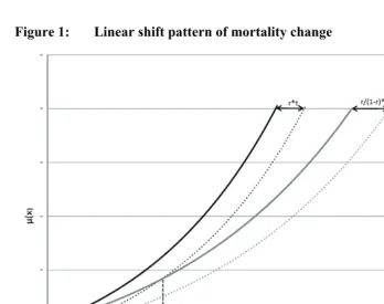
3.1 Linear shift pattern of mortality change
The linear shift pattern of mortality change is a pattern in which a baseline schedule of period mortality rates, µ(x, 0), is shifted every year along the age axis by a quantity r:
) 0 , ( ) ,
(xt =μ x−rt
μ . (4)
The linear shift assumption also assumes that µ(x,t)=0 for x<rt.
As a consequence of this shifting pattern in period mortality rates, the amount of shift for each successive cohort will be r/(1-r). Starting from a baseline schedule of cohort mortality rates, µc(x, 0):
) 0 , 1 ( ) ,
( t
r r x t
x C
c
− − =μ
μ (5)
and µc(x,t)=0 for x<r/(1-r)·t.
Figure 1: Linear shift pattern of mortality change
Rodriguez (2006:99-100) has shown that, with a linear shift for periods starting at time t=0, CAL will follow a linear trajectory:
rt
+
e t
CAL()= P(0)
0 (6)
where e0p(0) is the baseline life expectancy embodied in µ(x,0). He also showed that,
given a linear shift starting at time t=0, the cohort life expectancy at birth will also change linearly, but at a different rate rc = r/(1-r):
t r r r e t e
P C
− + − =
1 1
) 0 ( )
( 0
Combining Equations (6) and (7), Rodriguez (2006) finds that:
) (t
) (t
t e−ρ
)) ( (t e0 t e0
CAL + C = C (8)
Or, alternatively, that:
)) ( (
0 t CALt CAL
eC − = (9)
In other words under the linear shift assumption, the correspondence between CAL and LCLE is perfect. Goldstein (2006) and Wilmoth (2005) reach the same conclusion with somewhat different demonstrations. Note that this result is exact and does not involve any other assumptions besides the linear shift assumption described in Equation (4). Again no assumption is made about the shape of the mortality schedule.
We would like to note that the linear shift assumption described here generates a situation in which the period force of mortality is proportional to the concurrent age intensity of the constant-birth population, a situation which Bongaarts and Feeney’s refer to as the “proportionality assumption” (Bongaarts and Feeney 2003). However the proportionality assumption is a more general assumption which does not necessarily guarantee that CAL and LCLE will agree. For example, in Bongaarts and Feeney’s well-known “pill” scenario (i.e., a one-time shift in a cohort mortality happening for all cohorts at the same time), the proportionality assumption is met, but the linear shift assumption is not. There is no CAL-LCLE correspondence in this scenario. We will discuss this scenario and its implications later in the paper.
3.2 Gompertz pattern of mortality with constant log-linear decline
This is a simple model of mortality change in which age-specific mortality follows a Gompertz model with a constant rate of improvement over time:
x e t x α β
μ( , )= (10)
This model of mortality change is in fact quite similar to the linear shift assumption described above. Under this model, as in the linear shift model,
) 0 , rt ( ) ,
(xt =μ x−
μ (11)
where r= ρ/β.
One difference, however, with the linear shift described above is that mortality at ages x<rt is not equal to 0. There is some mortality at these ages, following Equation 10. As a result CAL does not increase exactly by an amount of ρ/β, but by a slightly smaller amount. Similarly e0c does not increase exactly by an amount of ρ/(β-ρ), as one
would expect under the linear shift assumption. Nonetheless the additional mortality existing under this scenario is small enough that Equations (6) and (7) can be approximated using r= ρ/β. (See Goldstein and Wachter (2006) for the details of this approximation.) Thus this Gompertz model will produce an approximate correspondence between CAL and LCLE, as Bongaarts and Feeney illustrated with their simulation. Figure 2 shows the difference between the model of mortality change described in this section, and a linear shift model in which mortality follows a Gompertz schedule.
Figure 2: Gompertz pattern of mortality with log-linear decline, and its
An interesting feature of these two models is that they produce a linear change in both CAL and LCLE, either exactly in the case of the linear shift assumption, or approximately in the case of the Gompertz model with constant log-linear decline.
4. Correspondence between CAL and LCLE in actual populations
4.1 Database
The data that we use in this paper come from the human mortality database (http://www.mortality.org). The number of country-years for which we can study the correspondence varies depending on the amount of historical data available and the choice of starting age for the calculation of life expectancies and CAL. In this paper we choose three starting ages: 0, 30, and 60. The number of country-years increases dramatically when using a starting age of 60.
4.2 Measurement issues
There are two ways of assessing the correspondence between CAL and LCLE in actual populations. The first option involves the comparison of e0c(t) vs. CAL(t+e0c(t)) for
each cohort born in year t. In a graph of CAL vs. LCLE, this difference amounts to the vertical difference between the two indicators. The second option involves comparing CAL(t) vs. e0c(t-CAL(t)) for each year t. In a graph of CAL vs. LCLE, this difference
amounts to the vertical projection of the diagonal difference between the two indicators. These two ways of representing discrepancies between CAL and LCLE can each be analyzed by period or by cohort. Thus there are four different ways of representing the correspondence between CAL and LCLE.
When the correspondence exactly holds, these various ways of representing the correspondence provide the same answer. When there is some discrepancy, however, the amount of discrepancy varies slightly depending on the choice of approach. Nonetheless the results are not substantially different, especially when CAL and cohort life expectancy are calculated on an annual basis.
the cohort currently reaching its life expectancy, we decided to study vertical differences by year. The existence of multiple vertical differences is rare enough in the mortality database that it can be disregarded in this empirical analysis.
Using age-specific death rates for each year and single-year age groups organized by cohorts, we calculated cohort survival probabilities for each annual cohort centered on January 1. These survival probabilities are then used to calculate cohort life expectancy for each cohort centered on January 1. These cohort survival probabilities are then summed cross-sectionally to calculate CAL for each year centered on January 1. The CAL series is then linearly interpolated to calculate the CAL value corresponding to each value of t+e0c(t). The difference between CAL(t+e0c(t)) and e0c(t)
can then be examined for each year at which CAL(t+e0c(t)) can be calculated.
When using a starting age other than 0, the CAL-LCLE correspondence is analyzed in a similar fashion. Defining t as the year at which a given cohort reaches age
x, we examine the correspondence between exc(t) and CAL
x(t+exc(t)).
4.3 Example: Swedish females
The top panel of Figure 3 shows trends in e0p, CAL
0, and LCLE0 among Swedish females. The bottom panel presents the difference between CAL0 and LCLE0 for the years when the two indicators overlap. During these years, the difference evolves from about -4 years to about +4 years.
Figure 3: Correspondence between CAL0 and LCLE0 among Swedish females
20
40
60
80
year
s
e0p LCLE_0 CAL_0
-4
-2
0
2
4
year
s
1750 1800 1850 1900 1950 2000
year CAL_0-LCLE_0
Source: The Human Mortality Database http://www.mortality.org
Figure 4: Correspondence between CAL30 and LCLE30 among Swedish females
20
30
40
50
60
year
s
e30p LCLE_30 CAL_30
-4
-2
0
2
4
year
s
1750 1800 1850 1900 1950 2000
year CAL_30-LCLE_30
The correspondence for life expectancy at age 60 is shown in Figure 5. At this age the correspondence is excellent. The difference is clearly centered around zero, with only very small deviations. There is no particular trend in the amount of difference.
Figure 5: Correspondence between CAL60 and LCLE60 among Swedish females
10
15
20
25
year
s
e60p LCLE_60 CAL_60
-4
-2
0
2
4
year
s
1750 1800 1850 1900 1950 2000
year CAL_60-LCLE_60
Source: The Human Mortality Database http://www.mortality.org
Figure 6: CAL/LCLE ratio among Swedish Females
.9
1
1.15 CAL_0/LCLE_0
.9
1
1.15 CAL_30/LCLE_30
.9
1
1.15
1800 1850 1900 1950 2000
year CAL_60/LCLE_60
Source: The Human Mortality Database http://www.mortality.org
4.4 Generalization
Figure 7: CAL0/LCLE0 ratio among countries in the human mortality database
Legend: De=Denmark; Fr=France; Sw=Sweden; F=Females; M=Males. Source: The Human Mortality Database http://www.mortality.org
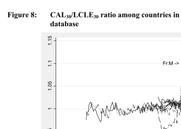
Figure 8: CAL30/LCLE30 ratio among countries in the human mortality
database
Fr:M ->
<- En:M <- It:M
.9
.95
1
1.05
1.1
1.15
1800 1850 1900 1950 2000
year
Legend: Fr=France; En=England & Wales; It=Italy; M=Males. Source: The Human Mortality Database http://www.mortality.org
Note: This figure includes data from the following countries (by sex): Denmark, France, England & Wales, Italy, Netherlands, New Zealand, Norway, Sweden, and Switzerland.
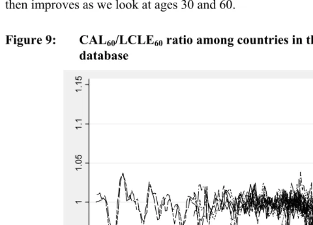
The correspondence is excellent with a starting age of 60 (Figure 9). We see oscillations around 1, with no particular pattern (except for a tendency for CAL60 to slightly underestimate LCLE60 towards the end of the period). For the country-years presented in the Figure 9, we find that CAL60 can be used as a precise proxy for cohort life expectancy at age 60 for the cohort reaching e60 in a given year.
ages has indeed shifted over time along the age axis in a somewhat linear fashion, especially after 1950. This helps explain why the correspondence is worse at age 0, and then improves as we look at ages 30 and 60.
Figure 9: CAL60/LCLE60 ratio among countries in the human mortality
database
.9
.95
1
1.05
1.1
1.15
1800 1850 1900 1950 2000
year
Source: The Human Mortality Database http://www.mortality.org
Note: This figure includes data from the following countries (by sex): Denmark, France, Finland, England & Wales, Italy, Netherlands, New Zealand, Norway, Spain, Sweden, and Switzerland.
5. Discussion
We find that the correspondence between CAL and LCLE holds exactly or approximately in a number of situations. It holds exactly under the constant shift assumption. It holds approximately under the Gompertz model with log-linear decline. The correspondence also holds extremely well for mortality above age 60 in all populations and time periods available in the human mortality database. Given the regularity of this finding across time periods and contexts, we find that when considering mortality above age 60, CAL provides an accurate estimate of the mean age at death for the cohort currently reaching its life expectancy. LCLE provides a useful way of representing cohort mortality, and we find that CAL can indeed be used as a shortcut for this representation above age 60. Thus the existence of an excellent CAL-LCLE correspondence at these ages provides an additional, concrete interpretation to CAL, an indicator which already has a number of known properties.
However we also find that the CAL-LCLE correspondence is not general. In particular the correspondence is somewhat less accurate at age 30, and far from accurate at age 0. This implies that when it comes to estimating lagged cohort life expectancy at birth or at age 30, CAL should not be used as a proxy. This means that there will be no alternative to mortality forecasts for estimating the current value of LCLE at birth. The mortality forecast approach to LCLE has the added advantage of making it clear what the assumptions are for the cohort’s future mortality.
As we said in the introduction the correspondence between CAL and LCLE was first observed in the literature on tempo effects in mortality. Indeed Bongaarts (2005) observed a correspondence, in the linear shift scenario and its Gompertz approximation, between their proposed measures of tempo-adjusted life expectancy (which include CAL, MAD, and M4) and LCLE. Although they do not propose LCLE as an indicator of tempo-adjusted life expectancy, they interpret this correspondence as a piece of evidence, in the linear shift scenario, that current period life expectancy overestimates life expectancy under current mortality conditions, and that their tempo-adjusted life expectancy corrects for this bias. The logic behind this conclusion is based on a parallel with fertility analysis where lagged cohort indicators are often used. Specifically the TFR for the cohort reaching its mean age at childbearing at time t is often compared to the period TFR at time t to assess the scale of tempo effects (Ryder 1980; Schoen 2004).
representation of changes in cohort completed fertility in a way that is more timely than its unlagged counterpart, yet not distorted by changes in the mean age at childbearing like the period TFR (Schoen 2004).
With their tempo-adjusted life expectancy, Bongaarts and Feeney are following a different route. They do not seek to better capture trends in cohort life expectancy. They seek to capture a life expectancy that better reflects underlying period mortality conditions. While CAL and LCLE are equal to one another under the linear shift scenario, they address two drastically different goals in the tempo literature: measuring period conditions vs. tracking cohort behavior.
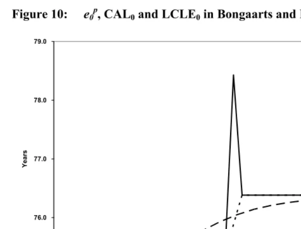
Figure 10: e0p, CAL0 and LCLE0 in Bongaarts and Feeney’s single shift scenario.
75.0 76.0 77.0 78.0 79.0
1950 1960 1970 1980 1990 2000 2010 2020 2030 2040 2050 Year
Y
ear
s
e0p LCLE CAL
LCLE is useful in other respects. In particular associating cohort life expectancy with its corresponding mean year at death is a useful way of summarizing many years of mortality influences, spanning the entire life course of a cohort. However average year at death for a given cohort appears to have little to do with the underlying mortality conditions of that year.
6. Acknowledgements
References
Bongaarts, J. (2005). Five measures of period longevity. Demographic Research
13(21): 547-558. doi:10.4054/DemRes.2005.13.21.
Bongaarts, J. and Feeney, G. (2003). Estimating mean lifetime. Proceedings of the National Academy of Sciences 100(23): 13127–13133. doi:10.1073/ pnas.2035060100.
Bongaarts, J. and Feeney, G. (2006). The quantum and tempo of life-cycle events.
Vienna Yearbook of Population Research 2006: 115–151. doi:10.1553/populationyearbook2006s115.
Brouard, N. (1986). Structure et dynamique des populations. La pyramide des années à vivre, aspects nationaux et exemples régionaux. Espaces, Populations, Sociétés
(2): 157–168.
Goldstein, J. (2006). Found in translation: A cohort perspective on tempo-adjusted life expectancy. Demographic Research 14(5): 71–84. doi:10.4054/ DemRes.2006.14.5.
Goldstein, J. and Wachter, K. (2006). Relationships between period and cohort life expectancy: Gaps and lags. Population Studies 60(3): 257-269. doi:10.1080/00324720600895876.
Guillot, M. (1999). The period average life (PAL). Paper presented at the PAA annual meeting, New York City, USA, March 25-27, 1999.
Guillot, M. (2003). The cross-sectional average length of life (CAL): A cross-sectional mortality measure that reflects the experience of cohorts. Population Studies
57(1): 41–54. doi:10.1080/0032472032000061712.
Guillot, M. (2005). The momentum of mortality decline. Population Studies 59(3): 283–294. doi:10.1080/00324720500223427.
Guillot, M. (2006). Tempo effects in mortality: An appraisal. Demographic Research
14(1): 1-26. doi:10.4054/DemRes.2006.14.1.
Keilman, N. (2006). Demographic translation: From period to cohort perspective and back. In: Wunsch, G., Caselli, G., and Vallin, J. (eds.). Demography: Analysis and Synthesis. Burlington, San Diego, and London: Elsevier: 215-225.
Ryder, N. (1980). Components of temporal variations in American fertility. In: Hiorns, R.W. (ed.). Demographic Patterns in Developed Societies. London: Taylor & Francis: 15-54.
Schoen, R. (2004). Timing effects and the interpretation of period fertility. Demography
41(4): 801-819. doi:10.1353/dem.2004.0036.
Wachter, K. (2005). Tempo and its tribulation. Demographic Research 13(9): 201–222. doi:10.4054/DemRes.2005.13.9.
Wilmoth, J. (2005). On the relationship between period and cohort mortality.