Analysis of Vector Estimating Modulation Method to
Eliminate Common Mode Voltage
N. Rashidirad
i; A. Rahmati
iiand A. Abrishamifar
iiiReceived 17 Mar 2012; received in revised 28 Sep 2012; accepted 15 Oct 2012
A
BSTRACTThe problem of common mode voltage in inverters can be considered as a major issue which leads to
motor bearing failures. To eliminate these voltages, proposing some methods seems to be necessary. This
paper has a comparative study on estimating modulation methods of eliminating common mode voltage. The
main idea of these methods is based on generation of reference vector with nearest vector/ vectors with zero
common mode voltage. Depending on the number of delivering nearest vectors, there are two estimating
methods. For the reference method, reference vector is synthesized only by the nearest vector. But for the
proposed method, the reference vector is synthesized by more than one vector. Dwell time calculations of
these vectors are based on the distance between the afore-mentioned vectors and the reference vector. In this
paper, some characteristics such as linear relationships among output voltage and modulation index, and
also total harmonic distortion of output voltage and stator current are considered. Finally, it is concluded
that the new method has more advantages such as more linear relationships and lower THD of current with
respect to the reference method.
K
EYWORDSCommon Mode Voltage, Modulation, Harmonic Distortion, Modulation Index
i * Corresponding Author,N. Rashidirad is with the Department of Electrical Engineering, Iran University of Science and Technology, Tehran, Iran (e-mail: [email protected])
iiA. Rahmati is with the Department of Electrical Engineering, Iran University of Science and Technology, Tehran, Iran (e-mail: [email protected]) iiiA. Abrishamifar is with the Department of Electrical Engineering, Iran University of Science and Technology, Tehran, Iran, (e-mail:
1. INTRODUCTION
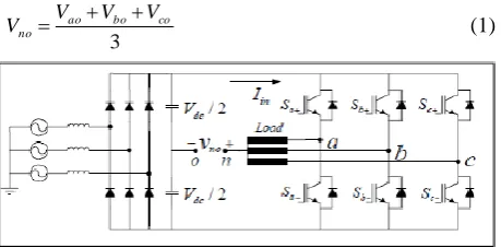
The problem of common‐mode voltage generation in an inverter-fed ac machine has been studied in the last two decades [1‐3]. Considering figure 1 that shows circuit configuration of an inverter, common mode voltage can be defined as:
(1) 3
co bo ao no
V V V
V
Figure 1: Circuit configuration of an inverter to define common mode voltage.
This voltage can lead to some problems in motor and its operations. The common‐mode voltage enables motor
shaft voltage to build up through electrostatic couplings between the rotor and the stator windings and between the rotor and the frame [4].
As the coupling currents find their way via the motor bearings, they form the so‐called bearing currents which have been shown in figure 2. When the shaft voltage exceeds the dielectric capability of the bearing grease, result in excessive currents that may cause bearing failures [2].
To reduce this voltage there are different solutions. Some solutions are based on additional hardware, like filters and other solutions are based on advanced modulation strategies which avoid the generation of common mode voltages. Among them SVM, due to its simplicity in hardware, software and reducing common mode voltage is more popular [4‐5].
2. CONVENTIONAL SVMALGORITHM
Since there are n distinct switching states for each phase of an n-level inverter, the total number of switching
states is
n
3 (which are the three-phase voltages in theabc
frame). In this format each switching state is represented by(
i
,
j
,
k
)
[
0
,
1
,
...,
n
1
]
and can defineappropriate connection of switches of the three phases. A set of balanced three-phase voltages in
abc
frame can be transformed into a two-dimensional
complexframe by the following transformation:
c b a
v
v
v
v
v
2
/
3
2
/
3
0
2
/
1
2
/
1
1
(2)
Applying this transformation, the switching voltage vectors in the
plane, form an (n-1) layer hexagoncentered at the origin of the
plane and also n zerovoltage vectors at the origin.
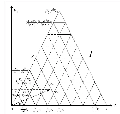
Figure 3: Representation of space voltage vectors of an n-level inverter in plane.
The hexagon is divided into six 60 degrees sectors and
each sector includes
(
n
1
)
2triangles.Projection of three-phase reference voltages into the new plane is a vector called the reference voltage vector,
ref
V
. This voltage has a constant magnitude and rotatescounterclockwise with a constant angular frequency. The SVM method is a discrete type of modulation technique. By this method, the reference vector is synthesized by the time average of a number of appropriate voltage vectors.
When the reference vector is located in one sector, it will lie in a specified triangle. As shown in figure 4, each triangle is formed by the three switching vectors adjacent to it. Therefore, these vectors are the best set of vectors to synthesize the reference vector which lies in the triangle. Therefore, the dwell times of the switching voltage vectors adjacent to the reference vector of an n-level inverter can be calculated as:
S ref j
j j j j
j
T
p
T
p
T
V
T
p
,1 ,1
,2 ,2
.
(3)S j j
j
T
T
T
T
,1
,2
(4)ref j
ref
ref
V
e
V
V
,
(5)dc ref
V
V
m
3
2
(6)
where
T
S is the switching period, m is the modulationindex,
p
j,p
j,1 andp
j,2 are the three voltage vectorsadjacent to the reference vector, and
T
j,T
j,1andT
j,2arethe calculated duty cycles of the voltage vectors, respectively [9].
Therefore, it can be concluded that calculations needed to synthesize the reference vector in the conventional SVM strategy can be classified into three steps.
The first step is based on identification of the sector and also the triangle in which the reference vector is located. The second step is to select the appropriate switching voltage vectors and finally the third step is to calculate dwell times of voltage vectors. Furthermore, as triangles change, the equations used for the calculations will be changed. In other words, each triangle has its own equations for calculation.
Therefore, as the number of levels of an inverter increases, the number of triangles and consequently the computations and also the complexity of calculations will increase. On the other hand, multilevel voltage source inverters offer several advantages compared to their conventional two-level inverters. In these inverters, by synthesizing several levels of dc voltages, the staircase output waveform is produced. The structure of this waveform will have lower total harmonic distortion which leads to a desired sinusoidal waveform. Achieving a higher output voltage and also a lower stress on power switches are other advantages of these inverters [6], [9].
As we know the problem of common mode voltage in multilevel inverters which had been found in conventional two level inverters can still be considered as a major issue which leads to motor bearing failure.
Therefore, proposing easier modulation methods based on space vector modulations to eliminate common mode voltage in multilevel inverters seems to be necessary.
3. VECTOR ESTIMATION METHODS
In inverters with an odd number of levels there is always a middle level that is called zero level. Due to this level in inverters with an odd level, there are switching sates with zero common mode voltage. Therefore, one of the easiest modulation methods with simple calculations to eliminate common mode voltage is to deliver nearest zero common mode voltage vectors.
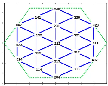
In the case of even level inverters, due to absence of switching states with zero common mode voltage, this strategy cannot be applied. Therefore, achieving elimination of common mode voltage in even level inverters is impossible. Figure 5 shows all zero common mode voltage vectors for a five level inverter. Since this estimation is based on restriction of voltage vectors, linear relationship will decrease [1, 8].
-4 -3 -2 -1 0 1 2 3 4 -4
-3 -2 -1 0 1 2 3 4
321 330
420
411
402 303 204 213 114 123
222 312 231 240 141
132 042
033
024
Figure 5: Voltage vectors with zero common mode voltage for a five-level inverter.
As it was mentioned, the number of switching states in
a three phase n-level inverter will be
n
3. Among these states, the number of voltage vectors in the space vector diagram will be calculated based on the following relations [7]:1
) 1 (n
Vn
(7)further,
)
1
(
6
) 1 ( )
(
n
n
n
V n V n (8)Therefore as shown in table 1, the number of voltage vectors with zero common mode voltage for a 5-level inverter is 19 vectors which have been shown in figure 5.
TABLE 1
RELATIONS BETWEEN NUMBER OF VECTORS AND SWITCHING
STATES
n
Number of Switching States in an n-level Inverter
Number of Voltage Vectors in an n-level Inverter
Number of Voltage Vectors withVcom=0 in
an n-level Inverter
1 1 1 1
3 27 19 7
5 125 61 19
7 343 127 37
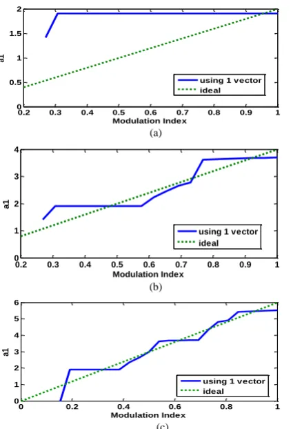
In this paper, the proposed method which leads to eliminate common mode voltage is known as a reference method. In higher level inverters the number of vectors with zero common mode voltage will increase. This increment leads to decrease the error of the generated voltage with respect to the reference voltage [1]. Figure 6 shows fundamental voltage versus modulation index in a 3-level, 5-level, and 7-level inverter. Therefore, as shown the linear relationship will improve.
0.2 0.3 0.4 0.5 0.6 0.7 0.8 0.9 1 0 0.5 1 1.5 2 Modulation Index a1
using 1 vector ideal
(a)
0.2 0.3 0.4 0.5 0.6 0.7 0.8 0.9 1 0 1 2 3 4 Modulation Index a1
using 1 vector ideal
(b)
0 0.2 0.4 0.6 0.8 1 0 1 2 3 4 5 6 Modulation Index a1
using 1 vector ideal
(c)
Figure 6: Fundamental voltage versus modulation index in a (a) 3-level, (b) 5-level, (c) 7-level inverter.
The main idea of the new vector estimating method is to deliver 2 or 3 nearest vectors to the reference vector. Identification of the nearest vectors can be achieved by comparison of calculated distances between the reference vector and each of the nearest vectors.
It should be noted that for the reference vector we have:
)
Im(
)
Re(
ref refref
V
j
V
V
(9)Furthermore, for each of the nearest vectors named as
k
V
, we have:3
,
2
,
1
),
Im(
)
Re(
V
j
V
k
V
k k k (10)In order to calculate the distances, the following equation is used:
2
2)
Im(
)
Im(
)
Re(
)
Re(
ref k ref kk
V
V
V
V
d
(11)To express the reference vector by these vectors dwell times of them are required. As we know, if one vector will be nearer to the reference vector, its dwell time will be longer. Furthermore, since for the nearest vectors method we have:
S
T T
T1 2 (12)
For the 3 nearest vectors method we also have:
S
T T T
T1 2 3 (13)
For a constant
T
S, (depending on the switchingfrequency), by increasing one dwell time, the others will
decrease. Therefore, if the reference vector is very close
to one of the estimated vectors (for example
V
1), it isexpected that the dwell time(s) of the other vector(s) will be negligible.
In other words, in this method the distance between the reference vector and each vector has a reverse relation with its dwell time. Hence the equations for using 2 nearest vectors become:
S T d d d T 2 1 2 1 (14) S T d d d T 2 1 1 2 (15)
And the equations for using the 3 nearest vectors are:
(16) S T d d d d d d T 3 2 1 1 3 2 1 (17) S T d d d d d d T 3 2 1 2 3 1 2 (18) S T d d d d d d T 3 2 1 3 2 1 3
where
T
1,T
2andT
3 are the dwell times of the threenearest voltage vectors to the reference vector, and
also
d
1,d
2 andd
3are the distance between each vectorand the reference vector.
Figure 7 shows the algorithm flowchart of the new estimation method (utilizing 2 nearest vectors). It is important to consider that selected values for a and b should be greater than the afore-mentioned nineteen distances.
4. SIMULATION RESULTS
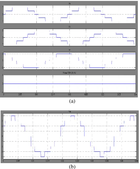
Figures 8 and 9 represent the phase voltages, line to line voltage, and common mode voltage in the five‐level inverter controlled respectively by the reference and the new (2 nearest vectors) estimation methods operating with a modulation index of m=.9 and fundamental frequency of 50Hz.
As expected, both of the estimation methods can eliminate the common mode voltage. But to have a better comparison, linear relationship and also THD will be studied in the next sections.
(a)
(b)
Figure 8: (a) phase and common mode voltages, (b) line to line voltage in the 5-level inverter by the reference method.
(a)
(b)
Figure 9: (a) phase and common mode voltages, (b) line to line voltage in the 5-level inverter by the new estimation method.
A. Linear Relationship Comparison
Figure 10 shows the comparison of fundamental voltage versus modulation index. Considering this figure it can be concluded that in the new modulation method, a better estimation of nearest voltage vectors will lead to a more linear relationship.
It should be noted that the proposed method with the three nearest vectors, in some ranges, has a negative slope. It means by increasing the modulation index in these ranges, fundamental voltage will decrease, which is assumed as a disadvantage. Therefore, using this method (three nearest vectors) is not recommended.
Furthermore, as is shown in figure 10, in the reference method the output voltage in the initial indexes is zero, which is undesired, while the proposed methods do not have this disadvantage.
B. THD Comparison
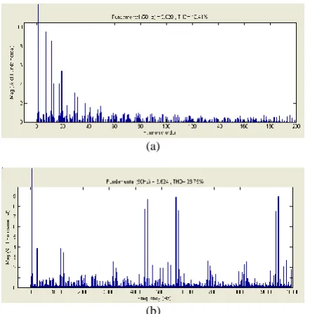
In this section, total harmonic distortions generated by new and reference estimation methods have been compared. Considering figure 11, which shows this comparison, it can be concluded that in the reference estimation method THD is less than that of the new estimation method. Moreover, considering figure 12, which shows line to line voltage spectrums, it can be concluded that in the new estimation method, the spectrum of line to line voltage has more high frequency components comparing with the reference method.
0.1 0.2 0.3 0.4 0.5 0.6 0.7 0.8 0.9 1 0
0.5 1 1.5 2 2.5 3 3.5 4
Modulation Index
a1
using 1 vector using 2 vectors using 3 vectors ideal
0.2 0.3 0.4 0.5 0.6 0.7 0.8 0.9 1 0
20 40 60 80 100 120 140 160 180 200
Modulation Index
%THD
using 1 vector using 2 vectors using 3 vectors
Figure 11: Comparison of total harmonic distortion (THD) versus modulation index (m) .
Appearance of these high frequency components can have an important role in THD comparison of stator currents. Figure 13 shows current spectrums for new and reference estimation methods. As shown in this figure, THD of stator current in the new estimation modulation method is less than that of the reference method.
(a)
(b)
Figure 12: Comparison of line to line voltage spectrum (a) in the reference estimation method and (b) in the new estimation method.
(a)
(b)
Figure 13: Comparison of current spectrum (a) in the reference estimation method and (b) in the new estimation method.
5. CONCLUSION
In this paper, two estimation modulation methods to eliminate common mode voltage have been compared. The difference between these methods is based on the number of delivering nearest voltage vectors. In this paper, to have a comparative study among these methods and the reference method some characteristics such as linear relationship and also total harmonic distortion have been considered.
In the new modulation method better estimation has led to decrement of the error of the generated voltage and improvement in linear relationship. Furthermore, because of high frequency components of the voltage spectrum, THD of stator current for the new method will be less than that of the reference one. Finally, it can be concluded that the new modulation method has more advantages such as a more linear relationship and a lower THD of current compared to the reference method.
6. ACKNOWLEDGMENT
7. REFERENCES
Periodicals:
[1] Jose Rodriguez, Jorge Pontt, Pablo Correa, Patricio Cortes, Cesar Silva, “A New Modulation Method to Reduce Common-Mode Voltages in Multilevel Inverters”, IEEE TRANSACTIONS ON INDUSTRY ELECTRONICS, VOL.51, NO.4, AUGUST 2004. [2] Shaotang Chen, Thomas A.lipo, Dennis Fitzgerald, “Modeling of
Motor Bearing Currents in PWM Inverter Drives”,IEEE TRANSACTIONS ON INDUSTRY APPLICATIONS, VOL. 32, NO. 6, NOVEMBER/ DECEMBER 1996.
[3] A. Muetze and A. Binder, “Don’t lose your bearings—Mitigation techniques for bearing currents in inverter-supplied drive systems,” IEEE Ind. Appl. Mag., VOL. 12, NO. 4, JULY/AUGUST 2006.
[4] Haoran Zhang, Annette von Jouanne, Shaoan Dai, Alan K.Wallace, Fei Wang, “Multilevel Inverter Modulation Schemes to Eliminate Common‐Mode Voltages”, IEEE TRANSACTIONS ON INDUSTRY APPLICATIONS, VOL. 36, NO. 6, NOVEMBER /DECEMBER 2000.
[5] Wenix Yao, Haibing Hu, Zhengyu Lu, “ Comparsions of Spacevector Modulation and Carrier-Based Modulation of Multilevel Inverter”, IEEE TRANSACTIONS ON POWER ELECTRONICS, VOL. 23, NO. 1, JANURAY 2008.
[6] Nasim Rashidirad, Abdolreza Rahmati, Adib Abrishamifar, “Comparison of Reliability in Modular Multilevel Inverters”, Electrical Review journal (PRZEGLAD ELEKTROTECHNICZNY), ISSN: 0033-2097, 2012
[7] Nasim Rashidirad, Abdolreza Rahmati, Adib Abrishamifar, “A Novel Scheme to Eliminate Common Mode Voltage in Multilevel Inverters”, International Journal of Scientific and Engineering Research, Jun 2011.
Papers from Conference Proceedings (Published):
[8] N. Rashidi‐ rad, A. Rahmati and A. Abrishamifar, “A New Modulation Method to Eliminate Common Mode Voltages in Modular Multilevel Inverters”, in Proc. 2011 IEEE International Conference on Information and Industrial Electronics, pp. 113-116.
Dissertations: