Accurate splitting approach to characterize the solution set of boundary layer problems

Accurate splitting approach to characterize the solution set of

bound-ary layer problems

Khosro Sayevand∗

Faculty of Mathematical Sciences, Malayer University, P. O. Box 16846-13114, Malayer, Iran.

E-mail: [email protected]

Jos´e Ant´onio Tenreiro Machado Institute of Engineering of Polytechnic of Porto, Department of Electrical Engineering, Porto, Portugal. E-mail: [email protected]

Abstract The boundary layer (BL) is an important concept and refers to the layer of fluid in the immediate vicinity of a bounding surface where the effects of viscosity are significant. This paper studies singularly perturbed fractional differential equations where the fractional derivatives are defined in the Caputo sense. The solution of such equations, with appropriate boundary conditions, displays BL behavior. The solution out of the BL is estimated by the solution of the reduced problem and the layer solution is approximated by means of a modified truncated Chebyshev series. The coefficients of the truncated series are evaluated using a novel operational matrix technique. Moreover, the stability and the error analysis of the proposed method are analyzed. Several examples illustrate the validity and applicability of the method.

Keywords. Singular perturbation, Boundary value problem, Shifted Chebyshev polynomial, Operational matrix, Boundary layer, Caputo fractional derivative.

2010 Mathematics Subject Classification. 26A33, 34K26, 34K10.

1. _Introduction

Singularly perturbed equations are ubiquitous in real-life phenomena and pose dif-ficulties for numerical approximations. Examples of application are geophysical fluid dynamics, oceanic and atmospheric circulation, chemical reactions, optimal control and many others [1]. We consider this type of problem where perturbations are op-erative over narrow regions across which the dependent variables undergo very rapid changes. These regions often adjoin the boundaries of the domain of interest, because a parameter with small numerical value multiplies the derivative of highest order. Such systems are referred, respectively as boundary, edge and skin layers in fluid mechanics, solid mechanics, and electrical applications respectively. We find many physical systems having sharp changes inside the domain of interest. The narrow regions where these changes occur are referred to as shock layers, in fluid and solid

Received: 26 January 2018 ; Accepted: 7 April 2019.

∗Corresponding author.

mechanics, transition points, in quantum mechanics, or Stokes lines and surfaces, in mathematics. The rapid variations cannot be handled by slow scales; however, they can be solved by means of fast, magnified, or stretched scales. For detailed discussion on the analytical and numerical treatment of such problems readers may refer to the works of O’Malley [15], Doolan et al. [5], Roos et al. [18], Nayfeh [12,13] and Miller et al. [10].

Fractional calculus (FC) has been in the mind of mathematicians during 300 years. In the last decades, FC became the object of increasing interest, due to its applications in different areas of science and engineering. Recently, it was verified that differential equations involving derivatives of non-integer order can model adequately various physical phenomena with long range memory effects [6,16]. The book by Oldham and Spanier [14] played a key role in the development of the subject. Some fundamental results related to fractional differential equations may be found in the seminal books of Miller and Ross [11], Kilbas et al. [9] and Baleanu et al. [2].

Despite the large number of studies dedicated to the solution of the singularly perturbed boundary value problems (e.g., Attili [1] and the survey by Kadalbajoo and Gupta [8]), we find only a few papers addressing fractional singularly perturbed boundary value problems (e.g., Bijura [4], Roop [17] and the references therein). Therefore, the topic remains an open area that deserves further research.

This paper focuses on the singularly perturbed boundary value problems of frac-tional order

ϵDmα_∗x y(x) +∑m

i=1fi(x, ϵ)D (m−i)α

∗x y(x) =g(x, ϵ), x∈[0,1], 0< α≤1,

(1.1)

with the boundary conditions

y(ik)_{(0) =a}

k, 0≤k≤i−1, y(jk)(1) =bk, 0≤k≤m−i−1, (1.2)

where i−1 < iα ≤ i, i = 1, . . . , m, and ϵ is a small parameter. The boundary conditions (1.2) constitute integer order derivatives ofy with respect to x, ik, jk ∈ {0,1, . . . , m−1}, with ik1̸=ik2 andjk1̸=jk2, ifk1≠ k2. Furthermore,fi(x, ϵ), i= 1, . . . , m, andg(x, ϵ) are continuous functions on [0,1]×[0, ϵ] andDiα

∗x,i= 0,1, . . . , m, denotes the Caputo fractional derivative that is defined in the follow-up.

stability analysis is performed considering the properties of the Mittag-Leffler func-tion. In section 4, the error of the method is analyzed. In section 5, some numerical examples are presented. Finally, section 6 outlines the concluding remarks.

2. _{Main idea of the method}

2.1. The shifted Chebyshev polynomial of the first kind. The main tool

to construct the spectral approximation of the layer solutions consists of the shifted Chebyshev polynomials. The shifted Chebyshev polynomial [3] of the first kindT_n∗(x), with degreenin x∈[0, δ], is defined by the relation

T_n∗(x) = cos (

ncos−1(2x

δ −1)

)

, n∈N, (2.1)

with following properties:

(i). Tn∗(x) has exactly nreal zeroes on the interval [0, δ]. The i-th zero of Tn∗(x) is located at

xi−1= δ

2 (

1 + cos

(_(n−i+1 2)π n

))

, i= 1,2, . . . , n. (2.2)

(ii). The relation between the powers xn and the shifted Chebyshev polynomials

Tn∗(x) is given by:

xn= δ n

22n₋1

n ∑

k=0 ′

( 2n

k

)

T_n∗_−k(x), (2.3)

where the prime indicates that the term fork= 0 to be halved.

2.2. Singularly perturbed boundary value problems. We consider the

gen-eral case of singularly perturbed boundary value problems with two BL (f1(x, ϵ) = 0,

for more details see [15]). It is straightforward to verify that this class of problems also contains problems includes also the case of a single BL. Let us first examine the reduced problem for (1.1)-(1.2)

∑m

i=1fi(x,0)D (m−i)α

∗x y0(x) =g(x,0), x∈[0,1], i−1< iα≤i, (2.4)

with the appropriate boundary conditions

y(ik)_{(0) =a}

k, 0≤k≤i−2, y(jk)(1) =bk, 0≤k≤m−i−2. (2.5)

The operatorDα

∗xy(x) represents the Caputo derivative which is defined by [7,19,20, 21]

1 Γ(n−α)

∫ x

0

(x−χ)n−α−1y(n)(χ)dχ, n−1< α≤n, n∈N, (2.6)

Problem (2.4)-(2.5) has the solution y0(x) which displays BL atx= 0 andx= 1.

Therefore, we seek a solution of (1.1)-(1.2) in the form

y(x)≈               

y1(x), x∈[0, δ],

y0(x), x∈[δ,1−γ],

y2(x), x∈[1−γ,1],

(2.7)

wherey1 andy2 are the layer functions satisfying

ϵDmα_∗x yς(x) + ∑m

i=1fi(x, ϵ)D (m−i)α

∗x yς(x) =g(x, ϵ), ς = 1,2, (2.8)

with the boundary conditions

y(ik)

1 (0) =ak, 0≤k≤i−1, (2.9)

y(ik) 1 (δ) =y

(ik)

0 (δ), 0≤k≤i−1, (2.10)

and

y(jk)

2 (1) =bk, 0≤k≤m−i−1, (2.11)

y(jk)

2 (1−γ) =y (jk)

0 (1−γ), 0≤k≤m−i−1. (2.12)

The parametersδ, γ >0 represent lengths of the layers are to be determined in the follow-up.

Let us now, construct the spectral approximation for the layer functiony1(x) and y2(x) in the form of truncated series

yςN(x) = N ∑

k=0

akTk∗(x), ς = 1,2, (2.13)

where ak, k = 0,1, . . . , N, are unknown coefficients, Tk∗(x), k = 0,1, . . . , N, are the shifted Chebyshev polynomials of the first kind andN is chosen any positive integer.

2.3. Fundamental matrix relations. In this section, we find the matrix forms

of terms and conditions of the Equations (2.8)-(2.12). We first consider the solution

yςN(x), ς = 1,2, and its derivatives D_∗kαxyςN(x) defined by a truncated Chebyshev series. Then, we can write series in matrix form

yςN(x) =T∗(x)A, D∗kαxyςN(x) =D∗kαxT∗(x)A, k= 0,1, . . . , m, ς= 1,2, (2.14)

where

T∗(x) = [T₀∗(x) T₁∗(x). . . T_N∗(x)], (2.15)

Dkα_∗xT∗(x) = [D_∗kα_xT₀∗(x), . . . , D_∗kα_xT₀∗(x)], (2.16)

Let us consider Equation (2.8) forς = 1. Consequently, one will set

T∗(x) =X(x)(DT)−1, (2.18)

where

X(x) = [1 x . . . xN], (2.19)

and D=            

δ020(0₀) 0 0 . . . 0

δ12−2(2₁) δ12−1(2₂) 0 . . . 0 δ2₂−4(4

2 )

δ2₂−3(4 3 )

δ2₂−3(4 4 )

. . . 0

. . . . . . . . . ._. . . . .

δN2−2N (_2N

N

)

δN2−2N+1 ( _2N

2N+1

)

δN2−2N+1 (_2N

N+2 )

. . . δN2−2N+1 (_2N

2N )             . (2.20)

Moreover, the relation between the matrixX(x) and its derivativeDkα_∗xX(x) is given by

Dkα_∗xX(x) =X−kα(x)Bk, (2.21)

where

X−kα(x) = [0· · ·0xj−kα· · ·xN−kα], k= 0,1, . . . , m, (2.22)

j = {

the largest integer such thatj≤[kα], kα∈N,

the largest integer such thatj−1≤[kα], kα̸∈N, (2.23)

and

Bk=           

0 . . . 0 0 . . . 0

..

. . .. ... ... . . . 0

0 . . . 0 0 . . . 0

0 . . . 0 _Γ((Γ(_j+1)j+1)_−kα) . . . 0 ..

. ... ... ... . .. ... 0 0 0 . . . 0 _Γ(Γ(_N+1N+1)_−kα)

          

, k= 0,1, . . ., m.

(2.24)

Using the relation (2.21), the derivative of the matrixT∗(x) defined in (2.18), can be expressed as

Dkα_∗xT∗(x) =D_∗kα_xX(x)(DT)−1=X−kα(x)Bk(DT)−1, k= 0,1, . . . , m, (2.25)

whereD0

∗xT∗(x) =T∗(x),X0(x) =X(x) andB0 is an identity matrixI. Substituting (2.25) into (2.14), we obtain

Dkα_∗xy1N(x) =X−kα(x)Bk(DT)−1A, k= 0,1, . . . , m, (2.26)

Using (2.26), the matrix form of the conditions given by (2.9)-(2.10) can be written as

y(ik)

1 (0) =ak=⇒X−ik(0)Bik(DT)−1A= [ak], (2.27)

y(ik) 1 (δ) =y

(ik)

0 (δ)=⇒X−

ik_(δ)Bik_(DT₎−1_{A= [y}(ik)

0 (δ)], (2.28)

where 0≤k≤I−1,and

X(0) = [1 0 · · · 0], (2.29)

X(δ) = [1 δ · · · δN], (2.30)

andX−ik _{is defined by (2.22).}

Let us consider Equation (2.8) for ς = 2. Then we can obtain the corresponding matrix relation as

T∗(x) =Z(x)(CT)−1, (2.31)

such that

Z(x) = [1 (x−1)· · ·(x−1)N], C=( C1 C2

)

, (2.32)

where

C1=

      

γ0₂0(0 0

)

0 −γ1₂−2(2

1

)

γ1₂−1(2 2

)

γ2₂−4(4 2

)

−γ2₂−3(4 3

)

..

. ...

(−1)N_γN₂−2N(2N N

)

(−1)N+1_γN₂−2N+1( 2N

2N+1

)       

, (2.33)

C2=

      

0 . . . 0

0 . . . 0

γ2₂−3(4 4

)

. . . 0

..

. . .. ...

(−1)N+2_γN₂−2N+1(2N N+2

)

. . . (−1)2N_γN₂−2N+1(2N

2N )

      

. (2.34)

Moreover, the relation between the matrixZ(x) and its derivativeD_∗kα_xZ(x) is

Dkα_∗xZ(x) =Z−kα(x)Bk, (2.35)

where

Z−kα(x) = [0· · ·0 (x−1)j−kα· · ·(x−1)N−kα], k= 0,1, . . . , m. (2.36)

Adopting (2.35), the derivative of the matrixT∗(x), defined in (2.31), can be expressed as

Dkα_∗xT∗(x) =D_∗kα_xZ(x)(CT)−1=Z−kα(x)Bk(CT)−1, k= 0,1, . . . , m, (2.37)

whereD0_∗xT∗(x) =T∗(x),Z0(x) =Z(x),B0=I. Substituting (2.37) into (2.14) leads to

whereD_∗0xy2N(x) =y2N(x).

Using (2.38), the matrix form of the conditions given in (2.11)-(2.12) can be written as

y(jk)

2 (1) =bk=⇒Z−jk(1)Bjk(CT)−1A= [bk], (2.39)

y(jk)

2 (1−γ) =y (jk)

0 (1−γ)=⇒Z−

jk₍₁−_γ)Bjk_(CT₎−1_{A= [y}(jk)

0 (1−γ)], (2.40)

where 0≤k≤m−I−1,and

Z(1) = [1 0 · · · 0], (2.41)

Z(1−γ) = [1 (−γ) · · · (−γ)N], (2.42)

andZ−jk _{is defined by (2.36).}

2.4. Method of solution. We can now construct the fundamental matrix

equa-tion corresponding to Equaequa-tion (2.8). For simplifying things, and without loss of generality, we assume that the boundary conditions are at most of first order deriva-tive. Substituting the matrix relation (2.26) into (2.8) forς = 1, we obtain

(

ϵX−mα(x)Bm(DT)−1+

m ∑

i=1

fi(x, ϵ)X−(m−i)α(x)B(m−i)(DT)−1 )

A=g(x, ϵ). (2.43)

For computing the Chebyshev coefficient matrixA, the zeroes of the shifted Cheby-shev polynomials of the first kind are substituted in Equation (2.43). Consequently, it yields

(

ϵX−mα(xi)Bm(DT)−1+ m ∑

i=1

fi(xi, ϵ)X−(m−i)α(xi)B(m−i)(DT)−1 )

A=g(xi, ϵ).

(2.44)

The fundamental matrix equation is given by: (

EX−mαBm(DT)−1+ m ∑

i=1

FiX−(m−i)αB(m−i)(DT)−1 )

A=G, (2.45)

where

Fi=     

fi(x0, ϵ) 0 0 . . . 0

0 fi(x1, ϵ) 0 . . . 0

..

. ... ... . .. ... 0 0 0 . . . fi(xN, ϵ)

   

, i= 1, . . . , m, (2.46)

X=     

1 x0 x20 . . . xN0

1 x1 x21 . . . xN1

..

. ... ... . .. ... 1 xN x2N . . . xNN

   

E=     

ϵ 0 0 . . . 0 0 ϵ 0 . . . 0

..

. ... ... . .. ... 0 0 0 . . . ϵ

   

, G=     

g(x0, ϵ) g(x1, ϵ)

.. .

g(xN, ϵ)    

. (2.48)

The fundamental matrix Equation (2.45) corresponds to a system of (N+ 1) algebraic equations for the (N+ 1) unknown coefficients {a0, a1, . . . , aN}. Therefore, we can write Equation (2.43) as

WA=G, or [W;G], (2.49)

so that, forp, q= 0,1, . . . , N, it yields

W= [wp,q] =EX−mαBm(DT)−1+ m ∑

i=1

FiX−(m−i)αB(m−i)(DT)−1. (2.50)

The matrix form for conditions (2.9)-(2.10) are

A0A= [a0], or [A0;a0], B0A= [a1], or [B0;a1], (2.51)

AδA= [y0(δ)], or [Aδ;y0(δ)], BδA= [y′0(δ)], or [B0;y′0(δ)], (2.52)

where

Ai=X(i)(DT)−1≡[ai0ai1· · ·aiN], i= 0, δ, (2.53)

Bi=X−1(i)B(DT)−1≡[bi0bi1· · ·biN], i= 0, δ. (2.54)

For obtaining the solution of Equation (2.8) under the conditions (2.9)-(2.10), we replace the rows matrices (2.51)-(2.52) by the first and last two rows of the matrix (2.49), respectively. Therefore, we have the augmented matrix

[W∗;Y∗] =             

w2,0 w2,0 . . . w2,N ; g(x2) w3,0 w3,1 . . . w3,N ; g(x3)

..

. ... . . . ... ... ...

w(N−2),0 w(N−2),1 . . . w(N−2),N ; g(xN₋2) a0,0 a0,1 . . . a0,N ; a0 aδ,0 aδ,1 . . . aδ,N ; y0(δ) b0,0 b0,1 . . . b0,N ; a1 bδ,0 bδ,1 . . . bδ,N ; y0′(δ)

            

, (2.55)

and the corresponding matrix equation

W∗A=Y∗. (2.56)

Ifrank(W∗) =rank[W∗;Y∗] =N+ 1, then we can write

Thus, the coefficientsai, i= 0, . . ., N, are uniquely determined by Equation (2.57). Similarly, substituting the matrix relation (2.37) into (2.8) forς= 2 we obtain

(

ϵZ−mα(x)Bm(CT)−1+

m ∑

i=1

fi(x, ϵ)Z−(m−i)α(x)B(m−i)(CT)−1 )

A=g(x, ϵ). (2.58)

The fundamental matrix equation is given by

(

EZ−mαBm(CT)−1+ m ∑

i=1

FiZ−(m−i)αB(m−i)(CT)−1 )

A=G, (2.59)

where

Z=     

1 (x0−1) (x0−1)2 . . . (x0−1)N

1 (x1−1) (x1−1)2 . . . (x1−1)N

..

. ... ... . .. ... 1 (xN −1) (xN −1)2 . . . (xN −1)N

   

. (2.60)

We can write Equation (2.58) as

WA=G, or [W;G], (2.61)

so that, forp, q= 0,1, . . . , N, we have

W= [wp,q] =EZ−mαBm(CT)−1+ m ∑

i=1

FiZ−(m−i)αB(m−i)(CT)−1. (2.62)

Furthermore, the matrix form for conditions (2.11)-(2.12) are

C1A= [a0], or [C1;b0], D1A= [b1], or [D1;b1], (2.63)

C1−γA= [y0(1−γ)], or [C1−γ;y0(1−γ)], (2.64)

D1−γA= [y0′(1−γ)], or [D1−γ;y0′(1−γ)], (2.65)

where

Ci=Z(i)(CT)−1≡[ci0ci1· · ·ciN], i= 1,1−γ, (2.66)

Di=Z−1(i)B(CT)−1≡[di0di1· · ·diN], i= 1,1−γ. (2.67)

(2.61) respectively, and we obtain the augmented matrix

[W∗;Y∗] =             

w2,0 w2,0 . . . w2,N ; g(x2) w3,0 w3,1 . . . w3,N ; g(x3)

..

. ... . . . ... ... ...

w(N₋2),0 w(N₋2),1 . . . w(N₋2),N ; g(xN−2) c1,0 c1,1 . . . c1,N ; b0 c1−γ,0 c1−γ,1 . . . c1−γ,N ; y0(1−γ)

d1,0 d1,1 . . . d1,N ; b1 d1−γ,0 d1−γ,1 . . . d1−γ,N ; y0′(1−γ)

            

. (2.68)

The corresponding matrix equation is:

W∗A=Y∗. (2.69)

Thus, the coefficientsai, i= 0, . . ., N, are uniquely determined by Equation (2.69).

3. _{Stability and error analysis}

In this section, the stability and error of the proposed method are analyzed based on properties of the Mittag-Leffler function and shifted Chebyshev polynomials.

3.1. On the asymptotic Mittag-Leffler stability.

Definition 1. The Mittag-Leffler function Eα,β(z)with α > 0,β >0 is defined by the following series representation, valid in the whole complex plane

Eα,β(z) = ∞ ∑

n=0 zn

Γ(nα+β), z∈C. (3.1)

Forβ= 1, we obtain the Mittag-Leffler function with one parameter:

Eα,1(z) = ∞ ∑

n=0 zn

Γ(nα+ 1) ≡Eα(z). (3.2)

It is to be noted that the fractional differential equation

dα_y

dxα =g(x, y), (3.3)

is asymptotic Mittag-Leffler stable if there exist positive constantskandλsuch that

|y(x)| ≤kEα(−λ(x−s)α), 0≤s≤t < ∞. (3.4) We consider the changes in the solution that are caused by small variations in the orderαand boundary conditions and functions fi(x, ϵ) andg(x, ϵ). Let us introduce small changes in problem (1.1)-(1.2) as follows:

ϵDm_∗xα˜y˜(x) +∑m i=1

˜

fi(x, ϵ)D_∗(mx−i) ˜αy˜(x) = ˜g(x, ϵ), x∈[0,1], 0< α≤1, (3.5)

with the boundary conditions

y(ik)_{(0) = ˜a}

Theorem 3.1. Ify(x)defined as (2.7) is a solution of the Equation (1.1) satisfying the boundary conditions (1.2), andy˜(x)is a solution of Equation (3.5) satisfying the conditions (3.6), then there exists a constantl such that the following relation holds:

y(x)≈y˜(x) +Emα ( l ϵx mα ) . (3.7)

Proof. Substitutingy(x) defined as (2.7) in Equation (1.1) and applying the operator

Iα

x, the inverse of the operatorDα∗x, to both sides of this equation yields

y(x) = m∑−1

i=0 cixi

i! + 1

ϵΓ(mα) ∫ x

0

(x−χ)mα−1 (

g(χ, ϵ)

− ∑m

i=1fi(χ, ϵ)D (m−i)α ∗χ y(χ)

)

dχ, (3.8)

where the constants ci can be determined by the boundary conditions (1.2). The same relation holds for ˜y. Therefore, we can write

|y(x)−y˜(x)| ≤ m∑−1

i=0

(ci−c˜i)xi

i!

+ 1

ϵΓ(mα) ∫ x

0

(x−χ)mα−1 (

g(χ, ϵ)− m ∑

i=1

fi(χ, ϵ)D

(m−i)α ∗χ y(χ)

−g˜(χ, ϵ) + m ∑

i=1

˜

fi(χ, ϵ)D

(m−i) ˜α ∗χ y˜(χ)

)

dχ

+ 1

ϵΓ(mα) ∫ x

0

(x−χ)mα−1 (

˜

g(χ, ϵ)− m ∑

i=1

˜

fi(χ, ϵ)D

(m−i) ˜α ∗χ y˜(χ)

)

dχ

− 1

ϵΓ(mα˜) ∫ x

0

(x−χ)mα˜−1 (

˜

g(χ, ϵ)− m ∑

i=1

˜

fi(χ, ϵ)D

(m−i) ˜α ∗χ y˜(χ)

)

dχ. (3.9)

We now consider the following relation:

_ϵΓ(1_mα) ∫ x

0

(x−χ)mα−1 (

g(χ, ϵ)− m ∑

i=1

fi(χ, ϵ)D_∗(mχ−i)αy(χ)

−g˜(χ, ϵ) + m ∑

i=1

˜

fi(χ, ϵ)D_∗(mχ−i) ˜αy˜(χ) )

dχ

= 1

ϵΓ(mα) ∫ x

0

(x−χ)mα−1 [(

g(χ, ϵ)− m ∑

i=1

fi(χ, ϵ)D_∗(mχ−i)αy(χ)

−g(χ, ϵ) + m ∑

i=1

fi(χ, ϵ)D_∗(mχ−i) ˜αy˜(χ) )

+

(

g(χ, ϵ)−

m ∑

i=1

fi(χ, ϵ)D_∗(mχ−i)αy(χ)−g(χ, ϵ) +˜ m ∑

i=1

˜

fi(χ, ϵ)D(_∗mχ−i) ˜αy(χ)˜ )]

Hence, we obtain

|y(x)−y˜(x)| ≤ m∑−1

i=0

|ci−c˜i|xi

i!

+ 1

ϵΓ(mα) ∫ x

0

(x−χ)mα−1|y(χ)−y˜(χ)|dχ+ 1

ϵΓ(mα) ∫ x

0

(x−χ)mα−1dχ

+sup˜g(χ, ϵ)− m ∑

i=1

˜

fi(χ, ϵ)D_∗(mχ−i) ˜αy˜(χ)× 1

ϵΓ(mα) ∫ x

0

(x−χ)mα−1dχ

− 1

ϵΓ(mα˜) ∫ x

0

(x−χ)mα˜−1dχ. (3.11)

Therefore, we conclude that

y(x)≈y˜(x) + l

ϵΓ(mα) ∫ x

0

(x−χ)mα−1|y(χ)−y˜(χ)|dχ. (3.12)

In summary, we have

y(x)≈y˜(x) +Emα (

l ϵx

mα )

. (3.13)

3.2. Error analysis for BL problems. Let y(x) and y1(x) be the solutions of

(1.1)-(1.2) and the boundary value problem (2.8)-(2.12), respectively. Then, we have:

Theorem 3.2. Consider problems with left BL. Ify1∈Cα+1[0,1], then the error on the BL[0, δ] can be estimated as follows

Ξ(x)≤Ξ1+ Ξ2, (3.14)

where

|y(x)−y1(x)| ≤C|y(δ)−y0(δ)|= Ξ1, (3.15) and

δα+1

22α+1_{(α+ 1)!}∥y (α+1)

1 ∥∞= Ξ2, n−1< α≤n, n∈N. (3.16)

Proof. First, consider the following definition:

”A real functiony(x), x >0, is said to be in the spaceCα, α∈R, if there exists a real numberp(> α), such thaty(x) =xp_y

c(x), whereyc(x)∈C[0,∞), and it said to be in the spaceCαn,n∈N∪ {0}, if and only if y(n)(x)∈Cα.”

Now, inside the BL, forx∈[0, δ] and based on (2.13), we have

Ξ(x)≤ |y(x)−y1(x)|+|y1(x)−y1N(x)|. (3.17)

Since∥T_k∗₊₁∥_∞= 1, we conclude that if we choose the grid nodes (xi)0≤i≤N, it comes

sup∥ k ∏

i=0

(x−xi)∥∞=

δα+1

In particular, for anyy1∈Cα+1[0,1] we have

∥y1−y1N∥∞≤

δα+1

22α+1_{(α+ 1)!}∥y (α+1)

1 ∥∞. (3.19)

By use of (3.19), forx∈[0, δ] it yields

Ξ(x)≤Ξ1+ Ξ2, (3.20)

and this proves Theorem3.2.

Proposition 1. The error estimate for x ∈ [1−γ,1] can be provided in the same manner.

4. _{Illustrative problems}

To demonstrate the applicability of the method, and to assess its performance we consider in the follow-up three problems. The examples are discussed in the literature for α = 1. In the last two cases, their exact solutions are available for comparison whenα= 1. The approximate solutions are calculated by means of the Maple software.

Example 1. Consider the following fractional singularly perturbed differential equa-tion

−ϵ2D_∗2αxy +

2 + 4ϵ2−2ϵ2x (2−x)2 D

α

∗xy=

ϵ2π2 (2−x)4cos

(

π(1−x) 2−x

)

+ 2π

(2−x)4 sin

(

π(1−x) 2−x

)

, (4.1)

i−1< iα≤i, i= 1,2, y(0) =y(1) = 0. (4.2)

Whenϵ→0, the order of the differential equation reduces to one and one of the boundary conditions must be dropped. It is clear that, the BL is at the right end, and the reduced equation satisfies the boundary conditiony(0) = 0. Hence, for sufficiently small ϵ, we have a thin BL on the right hand side, making it an ideal problem for application of the present method.

Forα= 1 (see[5]),ϵ= 0.1 andN = 5, the approximate solutions have the following form:

        

1−γ= 0.9802, y0=cos(π(1₂₋−_xx)),

y2= 0.5815T₀∗_,[1−γ,1]−0.5390T₁∗_,[1−γ,1]−0.1100T₂∗_,[1−γ,1]+ 0.0342T₃∗_,[1−γ,1]

+0.0276T₄∗_,[1−γ,1]+ 0.0057T₅∗_,[1−γ,1].

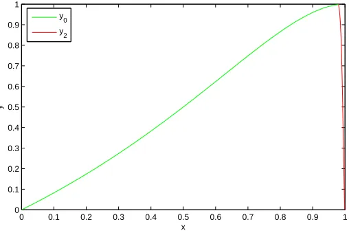
Figure 1. Numerical results for Example 1, when ϵ = 0.1, α = 1

andN = 5.

0 0.1 0.2 0.3 0.4 0.5 0.6 0.7 0.8 0.9 1 0

0.1 0.2 0.3 0.4 0.5 0.6 0.7 0.8 0.9 1

x

y

y₀

y 2

Example 2. Consider the following fractional singularly perturbed differential equa-tion

−ϵ2D_∗2xαy+y=−cos2(πx)−2(ϵπ)2cos(2πx), 1<2α≤2, (4.3)

y(0) =y(1) = 0. (4.4)

The order of the highest derivative is greater than the order of the second term. In this case there are two BL, one at each end.

For α = 1 (see [5]), ϵ = 0.01 and N = 5, the approximate solutions have the following form:

                    

δ=γ= 0.0630,

y0=−cos2(πx),

y1=−0.7476T0∗,[0,δ]−0.3708T1∗,[0,δ]+ 0.2322T2∗,[0,δ]−0.1005T3∗,[0,δ]

+0.0347T₄∗_,[0,δ]−0.0093T₅∗_,[0,δ],

y2=−0.7476T0∗,[1₋γ,1]−0.3708T1∗,[1₋γ,1]+ 0.2322T2∗,[1₋γ,1]−0.1005T3∗,[1₋γ,1]

+0.0347T₄∗_,[1−γ,1]−0.0093T₅∗_,[1−γ,1].

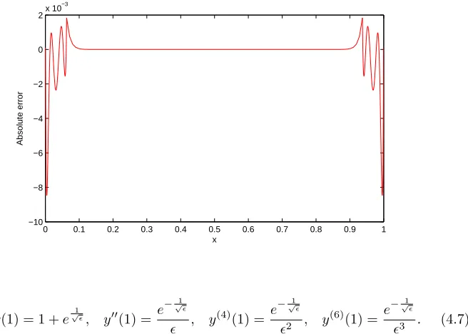
Example 3. Consider the following fractional singularly perturbed differential equa-tion

−ϵD8_∗α_xy+D_∗6α_xy−y=−x−e−√xϵ_{, i}−_{1< iα}≤_{i, i= 6,8, (4.5)}

y(0) = 1, y′′(0) =1

ϵ, y

(4)_{(0) =} 1 ϵ2, y

(6)_{(0) =} 1

Figure 2. Numerical results for Example 2, when ϵ= 0.01, α = 1

andN = 5.

0 0.1 0.2 0.3 0.4 0.5 0.6 0.7 0.8 0.9 1 −1

−0.9 −0.8 −0.7 −0.6 −0.5 −0.4 −0.3 −0.2 −0.1 0

x

y

y Exact(α=1) y₀

y 1 y

2

Figure 3. Absolute error for Example 2, whenϵ= 0.01, α= 1 and N = 5.

0 0.1 0.2 0.3 0.4 0.5 0.6 0.7 0.8 0.9 1 −10

−8 −6 −4 −2 0 2x 10

−3

x

Absolute error

y(1) = 1 +e√1ϵ_{, y}′′_{(1) =} e −_√1

ϵ

ϵ , y

(4)_{(1) =} e− 1

√_ϵ

ϵ2 , y

(6)_{(1) =} e− 1

√_ϵ

ϵ3 . (4.7)

Table 1. Numerical results for Example 2, when ϵ= 0.01, α = 1

andN = 5.

x yExact yOur method(N = 5) Absolute error

0.03 -0.941356556996480 -0.939137344081353 2.2192E-3 0.05 -0.968790311148491 -0.969804240304260 1.0139E-3

δ=0.0630 -0.959500065158029 -0.961336369935057 1.8363E-3

0.1 -0.904463097257711 -0.904508497187474 4.5399E-5 0.5 3.857499695890342E-22 -3.749399456654644E-33 3.8574E-22 0.9 -0.904463097257711 -0.904508497187474 4.5399E-5 1−γ= 0.9370 -0.959500065158029 -0.961336369935057 1.8363E-3 0.95 -0.968790311148491 -0.969804240304260 1.0139E-3 0.97 -0.941356556996480 -0.939137344081354 2.2192E-3

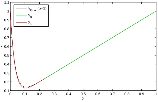
Figure 4. Numerical results for Example 3, when ϵ = ₂110, α = 1

andN = 8.

0 0.1 0.2 0.3 0.4 0.5 0.6 0.7 0.8 0.9 1 0.1

0.2 0.3 0.4 0.5 0.6 0.7 0.8 0.9 1 1.1

x

y

y Exact(α=1) y₀

y 1

For α = 1 (see [22]), ϵ = ₂110 and N = 8, the approximate solutions have the

following form: 

       

δ= 0.2339, y0=x,

y1= 0.3268T₀∗_,[0,δ]−0.2460T₁∗_,[0,δ]+ 0.2378T₂∗_,[0,δ]−0.1197T₃∗_,[0,δ]

Figure 5. Absolute error for Example 3, when ϵ= 2110, α= 1 and N = 8.

0 0.1 0.2 0.3 0.4 0.5 0.6 0.7 0.8 0.9 1 −2

0 2 4 6 8 10 12 14x 10

−3

x

Absolute error

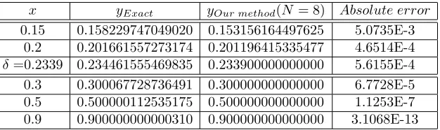
Table 2. Numerical results for Example 3, whenϵ=2110,α= 1 and N = 8.

x yExact yOur method(N = 8) Absolute error 0.15 0.158229747049020 0.153156164497625 5.0735E-3

0.2 0.201661557273174 0.201196415335477 4.6514E-4

δ=0.2339 0.234461555469835 0.233900000000000 5.6155E-4

0.3 0.300067728736491 0.300000000000000 6.7728E-5 0.5 0.500000112535175 0.500000000000000 1.1253E-7 0.9 0.900000000000310 0.900000000000000 3.1068E-13

5. _{Concluding remarks}

References

[1] B. S. Attili, Numerical treatment of singularly perturbed two point boundary value problems exhibiting boundary layers, Commun. Nonlinear Sci. Numer. Simul.,16(2011), 350-411. [2] D. Baleanu, K. Diethelm, E. Scalas, and J. J. Trujillo,Fractional calculus models and numerical

models (Series on Complexity, Nonlinearity and Chaos), Word Scientific, 2012.

[3] A. H. Bhrawy and A. S. Alo,The operational matrix of fractional integration for shifted Cheby-shev polynomials, Appl. Math. Lett.,26(2013), 25-31.

[4] A. M. Bijura, Nonlinear singular perturbation problems of arbitrary real orders, The Abdus Salam International Centre for Theoretical Physics, Trieste (Italy), 2003, 1-16.

[5] E. P. Doolan, J. J. H. Miller, and W. H. A. Schilders,Uniform numerical methods for problems with initial and boundary layers, Boole Press, Dublin, Ireland, 1980.

[6] O. Guner and A. Bekir,Solving nonlinear space-time fractional differential equations via ansatz method, Comput. Methods Differ. Equ.,6(1) (2018), 1-11.

[7] H. Jafari, H. Tajadodi, and D. Baleanu, A numerical approach for fractional order Riccati differential equation using B-spline operational matrix , Fract. Calculus Appl. Anal., 18(2) (2015), 387-399.

[8] M. K. Kadalbajoo and V. Gupta,A brief survey on numerical methods for solving singularly perturbed problems, Appl. Math. Comput.,217(2010), 3641-3716.

[9] A. Kilbas, H. M. Srivastava, and J. J. Trujillo,Theory and applications of fractional differential equations, Elsevier. Amsterdam, 2006.

[10] J. J. H. Miller, E. O’Riordan, and G. I. Shishkin,Fitted numerical methods for singular pertur-bation problems, World Scientific, Singapore, 1996.

[11] K. S. Miller and B. Ross,An introduction to the fractional calculus and fractional differential equations, John Willey and Sons, Inc. New York, 2003.

[12] A. H. Nayfeh,Introduction to perturbation techniques, Wiley, New York, 1993. [13] A. H. Nayfeh,Perturbation methods, Wiley, New York, 1973.

[14] K. B. Oldham and J. Spanier,The fractional calculus, Academic Press, New York, 1974. [15] R. E. O’Malley, Singular perturbation methods for ordinary differential equations, Springer

Verlag, New York, 1991.

[16] I. Podlubny,Fractional differential equations calculus, Academic Press, New York, 1999. [17] J. P. Roop,Numerical approximation of a one-dimensional space fractional advection-dispersion

equation with boundary layer, Comput. Math. Appl.,56(2008), 1808-1819.

[18] H. G. Roos, M. Stynes and L. Tobiska,Numerical methods for singularly perturbed differential equations, Springer, Berlin, 1996.

[19] A. Saadatmandi and M. Dehghan,A new operational matrix for solving fractional-order differ-ential equations, Comput. Math. Appl.,59(2010), 1326-1336.

[20] K. Sayevand and K. Pichaghchi, Successive approximation: A survey on stable manifold of fractional differential systems, Fract. Calc. Appl. Anal.,18(3) (2015), 621-641.

[21] J. A. Tenreiro Machado and V. Kiryakova,The chronicles of fractional calculus, Fract. Calc. Appl. Anal.,20(2) (2017), 307-336.