Almost periodic solution of a delayed Nicholson's blowflies model with feedback control

Commun. Math. Biol. Neurosci. 2015, 2015:10

ISSN: 2052-2541

ALMOST PERIODIC SOLUTION OF A DELAYED NICHOLSON’S BLOWFLIES

MODEL WITH FEEDBACK CONTROL

XIAOYING CHEN

Fuzhou University Zhicheng College, Fuzhou, Fujian 350002, China

Copyright c2015 Xiaoying Chen. This is an open access article distributed under the Creative Commons Attribution License, which permits unrestricted use, distribution, and reproduction in any medium, provided the original work is properly cited.

Abstract. In this paper, we study the problem of positive almost periodic solutions for the Nicholson’s blowflies mode with feedback control and multiple time-varying delays. By applying the properties of almost periodic function and exponential dichotomy of linear system as well as fixed point theorem, we establish the conditions for the existence uniqueness and exponential convergence of the positive almost periodic solution of the equations. Moreover, an example and its numerical simulation are given to illustrate our main results.

Keywords:Nicholson’s blowflies model; Positive almost periodic solution; Delay; Feedback control.

2010 AMS Subject Classification:34K14, 92D25.

1. Introduction

It is well known that the theory of Nicholson’s blowflies model has made a remarkable progress in the past forty years with main results scattered in numerous research papers; see, for example, [1-7] and the references cited therein.

In the real world, the delays in differential equations of population and ecology problems are usually time-varying. Recently, Chen and Liu [8] considered a class of the generalized Nicholson’s blowflies mode with multiple

∗_{Corresponding author}

E-mail address: [email protected] (X. Chen) Received December 15, 2014

time-varying delay as follows:

x0(t)−α(t)x(t) +

m

∑

βj(t)x(t−τj(t))e−γj(t)x(t−τj(t)), (1.1)

wheret ∈R, α,βj,γj,τj(j=1,· · ·,m):R→(0,+∞)are almost periodic functions. By constructing suitable Lyapunov functional, they showed that under a set of algebraic conditions, system (1.1) has a unique positive almost periodic solution. The solutions of this model converge exponentially to a positive almost periodic solution. On the other hand, ecosystem in the real world is continuously disturbed by unpredictable forces such as survival rates. Practical interest in ecology is the question of whether or not an ecosystem can withstand those unpredictable disturbances which persist for a finite period of time. In the language of control variable, we call the disturbance functions as control variables. Recently, some excellent results [9-12] which are concerned with existence and the stability of almost periodic solution of the single species or multi-species competition system with feedback control are obtained. However, to the best of the author’s knowledge, to this day, few work has dealt with the almost periodic solution of Nicholson’s blowflies models with feedback control and time-varying delays.

Motivated by the above, we consider the following generalized Nicholson’s blowflies model with feedback control and multiple time-varying delays:

x0(t) =−α(t)x(t) +

m

∑

βj(t)x(t−τj(t))e−γj(t)x(t−τj(t))−c(t)x(t)u(t−ζ(t)),

u0(t) =−λ(t)u(t) +g(t)x(t−δ(t)),

(1.2)

wherex(t)is a population size at timet,u(t)is the indirect control variable, andc(t),λ,g(t)are almost periodic functions. For convenience, we introduce the notations

f−=inf

t∈Rf(t), f

+_=sup

t∈R

f(t),

wheref is a continuous bounded function defined on[0,+∞). It will be assumed that

α−>0,β−_j >0,γ−_j >0,c−>0,λ−>0,g−>0,(j=1,· · ·,m)

and

τ+= max

1≤j≤m{sup_t∈R

τj(t)}>0,(j=1,· · ·,m),τ=max{τ+,ζ+,δ+}.

LetR2(R2+0)be the set of all (nonnegative) real vectors. DenoteC=C([−τ,0],R2)andC+=C([−τ,0],R2₊₀)as

the Banach space of continuous functions. Ifx(t),u(t)are defined on[t0−τ,σ)witht0,σ∈R1, then we defined Xt ∈CasXt= (x(t),u(t))wherext(θ) =x(t+θ),ut(θ) =u(t+θ)for allθ∈[−τ,0]. From the viewpoint of

mathematical biology, we consider (1.2) together with the following initial conditions

xt0=ϕ1,ut0=ϕ2,ϕ= (ϕ1,ϕ2)

T _∈

C+,ϕi(0)>0,i=1,2, (1.3)

We takeXt(t0,ϕ) =X(t,t0,ϕ)as a solution of the initial value problem (1.2) and (1.3) withXt0(t0,ϕ) =ϕ(t0∈

R). Also, let[t0,η(ϕ))be the maximal right-interval of existence ofXt(t0,ϕ).

2. Preliminaries

Definition 2.1(see [13]) Letx∈RnandQ(t)be an×ncontinuous matrix defined onR. The linear system

x0(t) =Q(t)x(t). (2.1)

is said to admit an exponential dichotomy onRif there exist positive constantsk,α, projectionPand the funda-mental solution matrixX(t)of (2.1) satisfying

kX(t)PX−1(s)k≤ke−α(t−s) _{for allt≥s,}

kX(t)(I−P)X−1(s)k≤ke−α(s−t) _{for allt≤s.}

Set

B={ϕ|ϕ= (ϕ1(t),ϕ2(t))Tis an almost periodic function onR}.

For anyϕ∈B, we define an induced modulekϕkB=sup t∈R

kϕ(t)k, theBis a Banach space.

Lemma 2.1(see [13])If the linear system (2.1) admits an exponential dichotomy, the almost periodic system

x0(t) =Q(t)x(t) +g(t). (2.2)

has an unique almost periodic solution x(t), and

x(t) =

Z t

−∞

X(t)PX−1(s)g(s)ds−

Z +∞

t

X(t)(I−P)X−1(s)g(s)ds. (2.3)

Lemma 2.2(see [13])Let ci(t)be an almost periodic function on R and

M[c_i] = lim

T→+∞ 1

T

Z t+T

T

ci(s)ds>0, i=1,2,· · ·,n.

Then the linear system

x0(t) =diag(−c1(t),−c2(t),· · ·,−cn(t))x(t),

admits an exponential dichotomy on R.

SetB∗={ϕ|ϕ∈B,k1≤ϕ1≤K1, k2≤ϕ2≤K2}.

Lemma 2.3(see [14])If u(t),g(t):R→R are almost periodic, then u(t−g(t))is almost periodic. We also suppose the following condition (H1) hold.

(H1)there exist four constants K1,K2,k1,and k2such that

K1>k1,K2>k2,K1>

m

∑

βj

γj

+ 1

α−e,

1 min

1≤j≤mγ

−

j

<k1<

m

∑

β−_j α+K1e

−γ+_jK1₋c

+_K

Lemma 2.4Let (H1) hold, and B∗={ϕ|ϕ∈B,k1≤ϕ1≤K1, k2≤ϕ2≤K2}. Then, forϕ∈B∗, the solution X(t,t0,ϕ)of (1.2) and (1.3) satisfies

k1<x(t,t0,ϕ1)<K1,k2<u(t,t0,ϕ2)<K2,for allt∈[t0,η(ϕ)) (2.4)

andη(ϕ) = +∞.

Proof.Setx(t) =x(t,t0,ϕ1). Let[t0,T)⊆[t0,η(ϕ)]be a interval such that

0<x(t) for allt∈[t0,T). (2.5)

We claim that

0<x(t)<K1for allt∈[t0,T). (2.6)

Assume, by way of contradiction, that (2.6) does not hold. Then, it existt1∈[t0,T)such that

x(t1) =K1and 0<x(t)<K1for allt∈[t0−τ,t1). (2.7)

Calculating the derivative ofx(t), from(H₁)and the fact that sup

u≥0

ue−u=1

e, the first equation of system (1.2) and

(2.7) yield that

0≤x0(t1) ≤ −α(t1)x(t1) +

m

∑

βj(t1)x(t1−τj(t1))e−γj(t1)x(t1−τj(t1))

≤ −α−x(t1) +

m

∑

βj(t1) γj(t1)

γj(t1)x(t1−τj(t1))e−γj(t1)x(t1−τj(t1))

≤ −α−x(t1) +

m

∑

βj

γj

+1 e

= α−−K1+

m

∑

βj

γj

+ 1 α−e

<0,

which is a contradiction and implies that (2.6) holds. In view ofu(t0) =ϕ2(0)>0, integrating the second equation

of (1.2) fromt0tot, we have

u(t) = e−

Rt

t₀λ(s)ds_u(t

0) +e

−Rt t₀λ(s)dsRt

t0e

Rs

t₀λ(ω)dω_{g(s)x(s−δ(s))ds} > 0, for allt∈[t0,η(ϕ)).

(2.8)

From (2.6) and (2.8), we obtain thatu(t)is bounded and there exist positive constantsK2such that

0<u(t)≤K2, for allt∈[t0,η(ϕ)). (2.9)

We next show that

x(t)>k1, for allt∈[t0,η(ϕ)). (2.10)

Otherwise, there existst2∈(t0,η(ϕ))such that

Then, from(H₁)and (2.6), we get

k1<x(t)<K1, γ+_j x(t)≥γ+_j 1

min

1≤j≤mγ

−

j

,for allt∈[t0−τ,t2), j=1,2,· · ·,m. (2.12)

Calculating the derivative ofx(t), together with(H1)and the fact that min

1≤u≤ω

ue−u=ωe−ω_{, the first equation of}

system (1.2), (2.11) and (2.12) imply that

0≥x0(t2) = −α(t2)x(t2) +

m

∑

βj(t2)x(t2−τj(t2))e−γj(t2)x(t2−τj(t2))−c(t2)x(t2)u(t2−ζ(t2))

≥ −α+x(t2) +

m

∑

βj(t2) γ+_j γ

+

j x(t2−τj(t2))e−γ +

jx(t2−τj(t2))_−c+_K

1K2

≥ −α+x(t2) +

m

∑

βj(t2) γ+_j γ

+

j K1e−γ +

jK1_−c+_K

1K2

= α+−k1+

m

∑

β−_j α+K1e

−γ+_j K1₋c

+_K

1K2 α+

>0,

which is a contradiction and yield that (2.10) holds. From (2.8) and (2.10), we obtain thatu(t)is bounded and there exist positive constantsk2such that

u(t)≥k2, for allt∈[t0,η(ϕ)). (2.13)

It follows from (2.6) (2.9) (2.10) and (2.13) that (2.4) is true. From Theorem 2.3.1 in [15], we easily obtain

η(ϕ) = +∞. This end the proof of Lemma 2.1.

3. Main results

Let

K2> g+K1

λ− , g−k1

λ+ >k2,max (

m

∑

j=1 β+_j α−e2 +

c+K2

α− + c+K1

α− , g+

λ− )

<1. (3.1)

Then, there exists a unique positive almost periodic solution of system (1.2) in the regionB∗.

Proof.For anyφ∈B, we consider an auxiliary equation



 

 

x0(t) = −α(t)x(t) +

m

∑

j=1

βj(t)φ1(t−τj(t))e−γj(t)φ1(t−τj(t))−c(t)φ1(t)φ2(t−ζ(t)), u0(t) = −λ(t)u(t) +g(t)φ1(t−δ(t)).

(3.2)

It follows from Lemma 2.3 thatφ1(t−τj(t)),φ1(t−δ(t)),φ2(t−ζ(t)),are almost periodic. Notice thatM[α]>

0, M[λ]>0, it follows from Lemma 2.2 that the linear equation







x0(t) = −α(t)x(t), u0(t) = −λ(t)u(t),

admits an exponential dichotomy on R. Thus, by Lemma 2.1, we obtain that the system (3.2) has exactly one almost periodic solution:

Xφ_{(t) = {x}φ_(t),uφ_(t)}

= nRt

−∞e −Rt

sα(u)du

m

∑

j=1

βj(s)φ1(s−τj(s))e−γj(s)φ1(s−τj(s))−c(s)φ1(s)φ2(s−ζ(s))

ds,

Rt

−∞e −Rt

sλ(u)du_{g(s)φ1(s−δ(s))ds}o_.

(3.4)

Define a mappingT :B→Bby setting

T(φ(t)) =Xφ_{(t), ∀}

φ∈B.

It is easy to see thatB∗is a closed subset ofB. For anyφ∈B∗, from (3.4) and sup

u≥0 ueu=1

e, we have

xφ_{(t) ≤} Rt

−∞e −Rt

sα(u)du

m

∑

j=1 βj γj +1 e ds

≤ ∑m

j=1

βj

γj + 1

α−e<K1,

uφ_{(t) ≤} Rt

−∞e −Rt

sλ(u)du_g+_K1ds=g

+_·K1

λ− <K2.

Noting thatk1>

1 min

1≤j≤mγ

−

j

and min

1≤u≤mue

−u_=me−m_{, we have}

xφ_{(t) ≥} Rt

−∞e −Rt

sα(u)du

m

∑

j=1

β_j−K1e−γ +

jK1_−c+_K

1K2

ds

≥ ∑m

j=1

β−_j K1e−γ+jK1

α− −

c+K1K2

α+ >k1,

uφ_{(t) ≥} Rt

−∞e −Rt

sλ(u)du_g−_k1ds=g

−_·k

1 λ+ >k2.

This implies that the mappingT is a self-mapping fromB∗toB∗.

Now, we prove that the mappingT is a contraction mapping onB∗. In fact, forφ,ψ∈B∗, we get

kT(φ)−T(ψ)kB=

sup

t∈R

| T(φ)(t)−T(ψ)(t) 1|,sup

t∈R

| T(φ)(t)−T(ψ)(t) 2|

sup

t∈R

| T(φ)(t)−T(ψ)(t)

1| = sup

t∈R

Rt

−∞e −Rt

sα(u)du

n m

∑

j=1 βj(s)

φ1(s−τj(s))e−γj(s)φ1(s−τj(s))

−ψ1(s−τj(s))e−γj(s)ψ1(s−τj(s))

−c(s)φ1(s)φ2(s−ζ(s))−ψ1(s)ψ2(s−ζ(s)) o

ds

Since sup

u≥1

|1−u

eu |=_e12, we obtain

|xe−x−ye−y| =

1−(x+θ(y−x)) ex+θ(y−x)

|x−y|

≤ 1

e2|x−y|, wherex,y∈[1,+∞),0<θ<1.

(3.5) combine with 1

min

1≤j≤mγ

+

j

<k1, we get

sup

t∈R

| T(φ)(t)−T(ψ)(t)₁| ≤

m

∑

j=1 β+_j

α−e2 kφ−ψkB +sup

t∈R

Rt

−∞e −Rt

sα(u)du_c(t)

φ1(s)φ2(s−ζ(s))−ψ1(s)φ2(s−ζ(s))|

+|ψ1(s)φ2(t−ζ(t))−ψ1(s)ψ2(s−ζ(s)) ds ≤ m ∑

j=1 β+_j

α−e2 kφ−ψkB+sup

t∈R

Rt

−∞e −Rt

sα(u)du_c(t)

K2

φ1(s)−ψ1(s)

+K1

φ2(s−ζ(s))−ψ2(s−ζ(s)) ds ≤ m ∑

j=1 β+_j

α−e2 kφ−ψkB+ c+K2

α− kφ−ψkB+ c+K1

α− kφ−ψkB

=

m

∑

j=1 β+_j α−e2 +

c+K2

α− + c+K1

α−

kφ−ψkB.

sup

t∈R

T(φ)(t)−T(ψ)(t)

2

= sup

t∈R

Rt

−∞e −Rt

sλ(u)du

g(s)φ₂(s−δ(s))−g(s)ψ2(s−δ(s)) ds ≤ sup

t∈R

Rt

−∞e −Rt

sλ(u)du_g+φ2(s−δ(s))−ψ2(s−δ(s)) ds

≤ g

+

λ−kφ−ψkB.

Hence

kT(φ)−T(ψ)kB≤max

(

m

∑

j=1 β_j+ α−e2

+c +_K2 α− +c +_K1 α− ,g + λ− )

kφ−ψkB.

Noting that

max

(

m

∑

j=1 β+_j α−e2 +

c+K2

α− + c+K1

α− , g+

λ− )

<1,

it is clear that the mappingT is a contraction onB∗. By the fixed point theorem of Banach space,T possesses a unique fixed pointφ∗∈B∗such thatTφ∗=φ∗. By (3.2),φ∗satisfies (1.2). Soφ∗is an almost periodic solution

of (1.2) inB∗. The proof of Theorem 3.1 is now complete.

Theorem 3.2. Let X∗(t)be the positive almost periodic solution of system (1.2) in the region B∗. Suppose that (3.1) holds. Then, the solution X(t;t0,ϕ)of (1.2) withϕ∈C converges exponentially to X∗(t)as t→+∞.

Proof.SetX(t) =X(t;t0,ϕ),z1(t) =x(t)−x∗(t)andz2(t) =u(t)−u∗(t), wheret∈[t0−τ,+∞). Then

          

z0₁(t) = −α(t)z1(t) +

m

∑

j=1

βj(t) x(t−τj(t))e−γj(t)x(t−τj(t))−x∗(t−τj(t))e−γj(t)x

∗_(t−

τj(t))

−c(t) x(t)u(t−ζ(t))−x∗(t)u∗(t−ζ(t)), z0₂(t) = −λ(t)z2(t) +g(t)z1(t−δ(t)).

Define a continuous functionΓ(µ)by setting

Γ(µ) =−(α−−µ) +

m

∑

β+_j 1 e2e

µ τ_,

µ∈[0,1].

Then, we have

Γ(0) =−α−+

m

∑

β+_j 1

e2<0, Γ(µ)→+∞(µ→+∞),

which implies that there exist two constantsη>0 andσ∈(0,λ−)∩(0,1]such that

Γ(σ) =−(α−−σ) +

m

∑

β_j+1 e2e

σ τ_<−

η<0. (3.7)

We consider the Lyapunov functional

V(t) =z1(t)eσt.

Calculating the upper right derivative ofV(t)along the solutionzt(t)of (3.6), we have

D+(V(t)) = −α(t)z1(t)eσt+

m

∑

j=1

βj(t) x(t−τj(t))e−γj(t)x(t−τj(t))−x∗(t−τj(t))e−γj(t)x

∗_(t−

τj(t))_eσt

−c(t) x(t)u(t−ζ(t))−x∗(t)u∗(t−ζ(t))eσt_+σz1(t)eσt

≤ h(σ−α(t))z1(t) +

m

∑

j=1

βj(t) x(t−τj(t))e−γj(t)x(t−τj(t))

−x∗(t−τj(t))e−γj(t)x

∗

(t−τj(t))i

eσt_{, for allt>t0.}

(3.8)

We claim that

V(t) =z1(t)eσt<eσt0

max

t∈[t0−τ,t0]

|ϕ1(t)−x∗(t)|+K1

:=M1, for allt>t0 (3.9).

Contrarily, there must existT1>t0such that

V(T1) =M1andV(t)<M1for allt∈[t0−τ,T1), (3.10)

which implies that

V(T1)−M1=0 andV(t)−M1<0 for allt∈[t0−τ,T1). (3.11)

Together with (3.5), (3.8) and (3.11), we obtain

0 ≤ D+(V(T1−M1)) = D+(V(T1))

≤ h(σ−α(T1))z1(T1) +

m

∑

j=1

βj(T1) x(T1−τj(T1))e−γj(T1)x(T1−τj(T1))

−x∗(T1−τj(T1))e−γj(T1)x

∗₍

T1−τj(T1)) i

eσT1

≤ (σ−α(T1))z1(T1)eσT1+

m

∑

j=1 βj(T1)

1

e2|z1(T1−τj(T1))|e

σ(T1−τj(T1))_eσ τj(T1)

≤ h−(α−−σ) +

m

∑

j=1 β+_j 1

e2e

σ τi_M1.

Thus,

0≤ −(α−−σ) +

m

∑

β_j+1 e2e

which contradicts with (3.7). Hence, (3.9) holds. It follows that

z1(t)<M1e−σt for allt>t0. (3.12)

Integrating the second equation of (3.6) fromT0tot(≥T0+τ), by (3.12), we get

z2(t) = e−

Rt

T₀λ(s)ds_{z2(T0) +}Rt

T0e

−Rt

sλ(v)dvg(s)z1(s−_δ(s))ds

≤ z2(T0)e−λ

−₍

t−T0)_+g+_M

1RTt0e

λ−(s−t)_e−σ(s−δ(s))_ds

= z2(T0)eλ

−_T

0_e−λ−t_+g+_M

1e−λ

−_tRt T0e

(λ−−σ)s_e−σ δ(s)_ds

≤ z2(T0)eλ−T0_e−λ−t₊g

+_M

1e−λ

−

t_eσ τ

λ−−σ e

(λ−−σ)t_−e(λ−−σ)T0

≤ z2(T0)eλ

−_T

0_e−λ−t₊g+M1eσ τ λ−−σ e

−σt

≤ z2(T0)eλ

−

T0_e−(λ−−σ)t₊g

+_M

1eσ τ λ−−σ

e−σt

≤ z2(T0)eλ

−_T 0₊g

+_M

1eσ τ λ−−σ

e−σt_.

LetM2=z2(T0)eλ−T0₊g

+_M

1eσ τ

λ−−σ , we have

z2(t)≤M2e−σt for allt>t0. (3.13)

It follows from (3.12) and (3.13) that the solutionX(t;t0,ϕ)of (1.3) converges exponentially toX∗(t)ast→+∞.

This completes the proof of Theorem 3.2.

4. An example

The following example shows the feasibility of our main results.

Example 4.1 Consider Nicholson’s blowflies model with feedback control:



   

   

x0(t) = −(19+cos2t)x(t) +ee−1(11+0.01|sin(√2t)|)x(t−e)e−x(t−e)

+ee−1_{(11+0.01|cos(}√_{3t)|)x(t−e)e}−x(t−e)₋ 1+t2

10+t2x(t)u(t−e−1),

u0(t) = −(1+0.1 cos4t)u(t) + (0.8+0.1|sint|)x(t−e−1).

(4.1)

Here corresponding to the system (1.2), we assume that

α−=19,α+=20, β_j−=11e−1, β_j+=11.01e−1,γ−_j =γ+_j =1,

c−=0, c+=0.1, τ=e>0, λ−=1,λ+=1.1, g−=0.9,g+=0.8,

and

2

∑

βj

γj

+ 1

α−e=2×11.01e

e−1 1

193 =2.377<e,

2

∑

β−_j α+K1e

−γ+_jK1₋c

+_K

1K2 α+ >2

11ee−1

20 ee

−e₋0.1e2

2

∑

j=1 β+_j α−e2 +

c+K2

α− + c+K1

α− =0.903<1, g+

λ−=0.9<1.

This implies that Nicholson’s blowflies model (4.1) satisfies the condition(H₁)and (3.1) withK1=K2=e,k1=

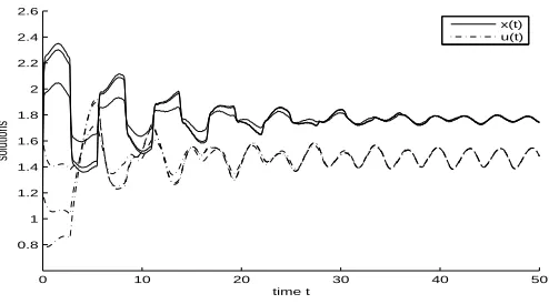
1, ,k2=0.5. Hence, from Theorem 3.1 and 3.2, system (4.1) has a positive almost periodic solution. Numeric

simulation (Fig. 1) strongly imply the above conclusion.

0 10 20 30 40 50

0.8 1 1.2 1.4 1.6 1.8 2 2.2 2.4 2.6

time t

solutions

x(t) u(t)

Fig. 1 Dynamic behavior of the solution(x(t),u(t))T of system (4.1) with the initial value

(ϕ₁(θ),ϕ1(θ))T= (1,0.8)T,(1.2,1.2)T and(1.6,1.6)T forθ∈[−τ,0], respectively.

Conflict of Interests

The author declares that there is no conflict of interests.

Acknowledgements

This work is supported by the Foundation of Fujian Education Bureau (JA13361) and the National Natural Science Foundation of Fujian Province (2013J01010).

REFERENCES

[1] K. Yang, X. D. Xie, F. D. Chen, Global stability of a discrete mutualism model, Abst. Appl. Anal. 2014 (2014), Article ID 709124.

[2] F. D. Chen, M. S. You, Permanence for an integrodifferential model of mutualism, Appl. Math. Comput. 186 (2007), 30-34.

[3] L. J. Chen, X. D. Xie, Feedback control variables have no influence on the permanence of a discrete N-species cooperation system, Discrete Dyn. Nature Soc. 2009 (2009), Article ID 306425.

[5] F. D. Chen, J. H. Yang, L. J. Chen, X. D. Xie, On a mutualism model with feedback controls, Appl. Math. Comput. 214 (2009), 581-587.

[6] L. J. Chen, L. J. Chen, Z. Li, Permanence of a delayed discrete mutualism model with feedback controls, Math. Comput. Modelling 50 (2009), 1083-1089.

[7] L. J. Chen, X. D. Xie, Permanence of an n-species cooperation system with continuous time delays and feedback controls, Nonlinear Anal. 12 (2001), 34-38.

[8] Y. K. Li, T. Zhang, Permanence of a discreteN-species cooperation system with time-varying delays and feedback controls, Math. Comput. Modelling 53 (2011), 1320-1330.

[9] X. D. Xie, F. D. Chen, Y. L. Xue, Note on the stability property of a cooperative system incorporating harvesting, Discrete Dyn. Nature Soc. 2014 (2014), Article ID 327823.

[10] X. D. Xie, F. D. Chen, K. Yang and Y. L. Xue, Global attractivity of an integrodifferential model of mutualism, Abst. Appl. Anal. 2014 (2014), Article ID 928726.

[11] K. Gopalsamy, X. Z. He, Persistence, attractivity, and delay in facultative mutualism, J. Math. Anal. Appl. 215 (1997), 154-173.

[12] X. P. Li, W. S. Yang, Permanence of a discrete model of mutualism with infinite deviating arguments, Discrete Dyn. Nature Soc. 2010 (2010), Article ID 93178.

[13] G. C. Sun, W. L. Wei, The qualitative analysis of commensal symbiosis model of two populations, Math. Theory Appl. 23 (2003), 64-68.

[14] M. Fan, K. Wang, Periodic solutions of a discrete time nonautonomous ratio-dependent predator-prey system, Math. Comput. Modell. 35 (2002), 951-961.