The Sustainable Development

Sustainable Development

Zahra Fotourehchi*1

Received: 2016, October 17 Accepted: 2016, December 13

Abstract

This research has aimed to examine the feedback effects between economic growth and environmental degradation through health that is one of human capital elements and also the consequences of such these relationships on economic convergence process during the period 1990-2013 for 60 developing countries in framework of simultaneous equations model by using imbalanced panel data analysis. This requires analyzing the interrelationships between economic growth, health, and environmental degradation. The results show the positive direct feedback effects between economic growth and health status, also positive indirect and reverse direct feedback effects between economic growth and environmental degradation. Although economic growth increases environmental degradation, sustaining the convergence process of developing countries and reaching the environmental Kuznets curve to turning point of CO2 emission represent stronger

indirect feedback effects between economic growth and environmental degradation than direct feedback effects.

Keywords: Economic Growth, Environmental Degradation, Health, Convergence, Sustainability

JELClassification: I10, Q56.

1. Introduction

Does economic growth increase or decrease environmental degradation? During the recent decades, many authors tried to give theoretical and empirical responses to this question and the most popular answer remains the Environmental Kuznets Curve Hypothesis (EKC). The EKC (Grossman and Krueger, 1991) describes the relationship between declining environmental qualities and increasing income as an inverted-U, in which environmental degradation increases until economic growth reaches a certain point, and then

decreases while the growth continues. However, the relationship between economic growth (income per capita) and environmental quality depends on scale, composition and technology effects. Environmental quality to worsen with increasing income, as greater output generates more pollution (the scale effect). On the other hand, environmental quality could improve with increasing income or the monotonic relationship between economic growth and environmental degradation could delink if this scale effect was eclipsed by the combination of both composition and technology effects. Line with increasing income per capita, the composition of output shifts from capital and pollution intensity based economies to information - technology/service based economics (the composition effect). Moreover, with increasing income transition from high polluting to low polluting technology leads to less environmental degradation (the technology effect). However, prior condition for EKC delinking is the increment of demand in the improvement of environmental quality that leads to the implementation of policies for environmental protection, also in the delinking process of EKC all said stages depend on sustainability of the increment of income.

One important critique for the existing empirical EKC studies is that although in the first stage of economic development, increasing income declines environment quality, there is no feedback effect from environmental degradation to economic growth and income rises continuously. However, the environmental degradation in turn can have significant effects on economic activity and economic growth (Bovenberg and Smulders 1995). The best way to understand how environmental degradation can affect economic growth is to explain the channels through which this occurs. In economic literature we can find implicitly or explicitly some of these channels. Most of the channel was met in the literature is the human capital especially health degradation.

Air pollutants such as CO2, SO2, NOx, CO, PM10 etc. affect health and leave people unable to work over short or long periods and reduce the productivity of those who work. This leads to declining quality and quantity of production/economic growth.

development and the potency of variant factors that affect on health status. Generally, it is assumed that health outcomes for a population improve when the economy grows (gains of growth), but degradations in the quality of environment and lifestyle (tendency to unhealthy and stressful life style) are generated line with economic growth adversely affect on health status (losses of growth). The gains and losses in health can cancel each other out and this challenges the idea that as income increases, health would always improve, this process also impacts on income simultaneously and leads to creating different types of feedback effects between economic growth/income and health.

At the same time, negative effect of environmental degradation on health status that restricts economic growth leads to indirect feedback effects between economic growth and environmental degradation, hence due to declining of income it is possible that EKC does not reach to its turning point.

The main goal of this research is the analysis of the feedback effects between economic growth and environmental degradation through health that is one of human capital elements and the consequences of considered relationships on economic convergence process during the period 1990-2013 for 60 developing countries. This requires examining the interrelationships between economic growth, health, and environmental degradation.

2. Materials & Methods

To highlight empirical analysis of the feedback effects between economic growth and environmental degradation through health, I combine three equations: Environment, health and economic growth equations for formulating Simultaneous Equations Models (SEM). Empirically, the SEM can be given as Eq. (1), (2) and (3):

 

it i0 i1 1it i2 1it i4 it 1it

e   α y α y   z  

it i i1 1it i2 2it i it i it i it 2it

lnh   α lny  lny  lns γ lne  lnw  

it i i, t i1 kit i2 it i3 it i4 it i t 3it

lny  lny _  1ns   lne   lnh   lnp       (1)

Where i=1, 2,..., N, and t=2τ,..., Tτ.

In this simultaneous regression model, environmental degradation

(e) is a function of economic growth (y1) and other determinant factors of environmental deterioration (z) like as educational level (s), urbanization (u), population density (p) and globalization (g). Health status (h) is a function of socio-economic factors like as economic growth (y1), health expenditure (y2), education level (s) and life style

(w). Economic growth (real GDP per capita) is a function of its lagged

value, (skit) which is the percentages of GDP saved and invested in the

physical capital, (eit) and (hit) which are the average proxies for

environmental and human capitals stocks and Pit which is the effective

labor force.

The first environment equation is reduced form of Environmental

Kuznets Curve (EKC) model. y1it2 denotes the sustainability of

environmental degradation, but if αi1<0 and αi2>0, there will be U link between them. Different from others I add globalization into environment equation to explain the impact of globalization on environmental degradation.

The second health equation is health production function that there are not implicit costs of environmental degradation.

The third economic growth equation is Solow (1956) neoclassical

growth model that has been extended by Knowles and Owen (1995)

through incorporating human capital (health and education) in the

model. Following Drabo (2010), I further extend this model by adding

environment quality to model (for more detail see appendix). The

coefficient of the lagged value of economic growth variable is expected to be superior to 0 and inferior to 1 (o<ƞ1<1) to confirm economic convergence hypothesis. I also expect βi2 to be inferior to 0.

3. Data

The data used in this paper are obtained from the World Development Indicators (2015), compiled by the World Bank and Global Information System on Alcohol and Health (GISAH) compiled by the World Health Organization. There are total 60 countries included in the analysis. 54% come from the upper middle-income and 46% are lower middle-income. In this paper for achieving consistent and robust results, I have used different proxy variables for human capital.

Proxy variable for the level of environment stock that is available for the analysis is carbon dioxide CO2 emission (metric tons per capita). This air pollutant through reducing air quality leads to decreasing quality and quantity of environment stock.

Like as previous studies (for example Knowles and Owen 1995;

McDonald and Roberts 2004), for the health stock level, I use life expectancy at birth proxy variable. Life expectancy at birth, (years) which is defined as the mean age at death of a fictitious generation subject to the mortality conditions of the period considered

(McDonald and Robert, 2004, p.8). I also use school enrollment,

secondary and tertiary (% gross) as proxies for education stock level which have been used in previous studies (for example webber, 2002;

McDonald and Robert, 2004).

GDP per capita (2005 constant dollar) for economic growth, gross

fixed capital formation (% of GDP) for the percentages of GDP saved

and invested in the physical capital and pi the sum of population

growth rate (ni), depreciation rate and technological progress

(g+δ=0.05) for workforce growth.

In the environmet equation proxy variables for population factors and globalization are population density (people per sq. km of land area), urban population (% of total) and KOF index, respectively. KOF index comprises social, economical and political aspects of globalization. In the health equation proxy variables for life style factor and health expenditure are alcohol per capita (15+) consumption and total per capita health expenditure, respectively. However, the use of health expenditures per capita may be had econometric problem of multicollinearity that arises from co-movement of health expenditures and GDP per capita. To reduce the possible effects of multicollinearity, like as the research of Fayissa

and Gutema (2005), I used the ratio of total health expenditure (y2) to

GDP (y1) as indicator for health expenditure per capita.

Before choosing an estimation method, the identification problem and choice of instruments of the nonlinear SEM should be mentioned. The identification problem for simultaneous equations models that are nonlinear in some endogenous variables is well discussed in Wooldridge (2002). The critical issue here is the choice of instruments for the quadratic term of GDP per capita. If the coefficient αi2 in Eq.(1) equals zero, then the model of Eqs. (1), (2), and (3) turns into a linear simultaneous equations system. In most linear simultaneous equations system, it is common to use all the exogenous variables in the system to be the instruments for all the endogenous variables. In the nonlinear case, a general approach is to also use some squares and cross products of the exogenous variables (Wooldridge, 2002, p. 235). From this view, the instruments for the quadratic term of GDP per capita are therefore chosen as all exogenous variables, their interaction and quadratic terms. After solving the instruments issue, the system in Eqs. (1), (2), and (3) can be studied using the usual rank and order conditions.

method used for estimating simultaneous equations models may be the best simple estimation method for the model in this paper. However, I prefer (3SLS) system estimation method to (2SLS) because of using full information in the system and considering both heteroskedasticity and contemporaneous correlation in the residuals (in the estimation unobserved heterogeneity among countries are not considered).

4.Results & Discussion

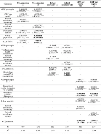
The results for the environment equation (see Tables 1 and 2) show that GDP per capita, different levels of education, urbanization, population density, as well as globalization significantly influence on CO2 emission. Furthermore, there is an inverse-U shaped EKC for

CO2 emission with turnig points between $7740-$8850 (GDP per

capita). The results further indicate that urbanization is positively related to CO2 emission, while population density and educational levels are inversely related to it. Hence, with increasing the percentage of population living in urban areas (urbanization), CO2 emission intesifies. In addition, as a country gets more crowded (more people on a fixed area of land/more population density), the higher will be their CO2 emission. This can be due to the fact that as population density increases, there are increasing pressure to use fossil fuel consumption and the existing land more intensively, but size squre. Km2 of land area in a country also has a significant role in the determination of impacts amount of population density on emission of pollutants. Especially, as the sample of the study (developing countries) has more land area, this leads to negative coefficient of population density.

said that in the formation of environmental policies for achieving efficient results line with the economic growth the effects of social and demographic factors on pollutants should not be ignored.

In the health equation, the coefficients of GDP per capita and health expenditure are found to be statistically significant, suggesting that both variables favorably influence health status. A higher level of income permits more access to consumption of higher quality of goods and services, better housing, and medical care services which favorably influence the health status, furthermore, increasing both per capita public and private health expenditure lead to higher health status.

Moreover, sections 2 of both Tables report that the coefficients of different levels of education have statistically positive impact on health status. This is possible as more education gives the people more awareness about their own health status and of what preventive measures may increase their own health.

Furthermore, the both Tables indicate that an increase in CO2 emission and per capita alcohol consumption contribute to the reduction of health status. Thus, it can be seen negative effect of per capita alcohol consumption on health status is very less than CO2 pollutant.

In general, the estimates suggest socio-economic factors (such as education levels, GDP per capita and health expenditure (in the Table 1) and GDP per capita, education levels and health expenditure (in the

Table 2), respectively) have stronger effects on health status than CO2

and alcohol consumption, respectively. However, health policies which focus on just socio-economic aspects and ignore the adverse impacts of CO2 emission may do little in efforts directed to improve the existing health status of the country, also may not deliver the full realizable health gains that can be derived from higher socio-economic levels.

In the economic growth equation, the coefficients on the lagged

value of GDP per capita and gross fixed capital formation (% of GDP)

are both positive and significant. These results are consistent with those of Mankiw, Romer and Weil (1992), Islam (1995) and McDonald and Roberts (2004).

negative although one of them is significant. For education, the regression results are also consistent with the theoretical predictions.

The coefficients on school enrollment, secondary and tertiary (%

gross) are all positive and significant. The positive sign indicates that the improvement in stock level of education increases economic growth. For the health stock proxy variables, the coefficients on life expectancy at birth and infant mortality are significantly positive and negative, respectively. Hence, increasing in life expectancy at birth and declining in infant mortality contribute to economic growth in the developing countries. These results are congruent with of those Knowles and Owen (1995) and McDonald and Roberts (2004).

However, coefficients on CO2 emission that reflect decreasing in

quality and quantity of environmental stock level are significantly negative. These results indicate that line with increasing air pollution emission in upper and lower middle income countries economic

growth declines.

Furthermore, general evaluation for the simultaneous equations model represents the positive direct feedback effects between economic growth and health and also positive indirect and negative direct feedback effects between economic growth and environmental degradation. Positive signs of coffiecients of economic growth and health variables in the health and economic growth equations show positive direct feedback effects between economic growth and health. Positive coffiecient of health in the economic growth equation is due to positive factors (GDP per capita, total per capita health expenditure, education levels) that affect on health (in the health equation) are stronger than negative factors (CO2 emission and Alcohol per capita (15+) consumption). This has creared positive direct feedback effect between economic growth and health.

Moreover, positive sign of cofficient of GDP per capita (proxy variable for the first stage of economic growth) in the environment equation and negative sign of cofficient of CO2 emission in the economic growth equation indicate that line with economic growth

increasing environmental degradation (the increment of CO2

Positive cofficient of intervening health variable in the economic growth equation also implies there is a positive indirect feedback effects between economic growth and environmental degradation. Although line with economic growth increasing environmental degradation negatively affects on health status, positive effect of health on economic growth has led to positive indirect (through health) feedback effects between economic growth and environmental degradation. On the other words, in the health equation, the effects (cofficients) of positive factors on health are stronger than negative factors. This has led to positive coffiecient of health in the economic growth equation and positive indirect feedback effects between economic growth and environmental degradation.

Generally, although economic growth increases environmental

degradation, sustaining the convergence process (convergence rates

take value between 0-1) of developing countries and reaching the

environmental Kuznets curve to turning point of CO2 emission

represent stronger indirect feedback effects between economic growth and environmental degradation than direct feedback effects.

5. Conclusion

Table1: 3SLS Estimation Results of SEM

Variables CO2 emission

(1)

CO2 emission

(2)

Life expectancy at birth (1)

Life expectancy at

birth (2)

GDP per capita (1) GDP per capita (2)

GDP per capita 0.000584 (5.7616) ***

0.000723

(6.6301) *** - - - -

(GDP per capita)2 _{(-3.0666) ***} -3.30E-08 _{(-4.1005) ***} -4.67E-08 - - - -

School enrollment, secondary

-0.03882

(-10.9112) *** - - - - -

School enrollment, tertiary -

-0.04582

(-9.2422) *** - - - -

Population density -0.002652 (-4.2503) ***

-0.0021

(-3.2226) *** - - - -

Urban population 0.01255 (2.6095) ***

0.0024

(0.4366) - - - -

KOF index _{(-2.1162) ***} -0.1605 _{(-1.94111) *} -0.0012 - - - -

GDP per capita - -

0.02449 (4.8842) ***

0.02387

(5.578838) *** - -

Total per capita health

expenditure - -

0.01621 (1.9277) *

0.01842

(2.8242) *** - -

School enrollment,

secondary - -

0.1653 (16.9441)

***

- - -

School enrollment,

tertiary - - -

0.08043

(21.097) *** - -

CO2 emission - -

-0.03191 (-3.3238) ***

-0.02368

(-4.4788) *** - -

Alcohol per capita

(15+) consumption - -

-0.001100 (-4.9459)

***

-0.00199

(-1.0711) - -

GDP per capita

(-1) - - - -

0.9873 (36.2611) ***

0.9848 (20.7668) *** Gross fixed capital

formation (% of GDP)

- - - - _{(5.1224) ***} 0.0350 _{(3.2222) ***} 0.0372

Workforce growth”

(ln(n+g+δ)) - - - - (-0.6744)-0.00227

-0.0014 (-1.9824) *

Life expectancy at birth - - - - _{(2.3112) **} 0.033051 _{(1.7325) *} 0.0858

School enrollment,

secondary - - - -

0.01602

(2.4222) ** - School enrollment,

tertiary - - - - -

0.0010 (1.8686) *

CO2 emission - - - - _{(-1.9778) *} -0.0019 _{(-2.2386) **} -0.0075

N 707 678 563 536 563 537

R2 _{0.59 0.54 0.64 0.55 0.99 0.99}

Note 1: Figures in the parenthesis indicate t-statistic. *%10, **%5 and ***%1 denote statistical significant level.

Table 2: 3SLS Estimation Results of SEM

Variables CO2 emission

(1)

CO2 emission

(2)

Infant mortality (1)

Infant mortality (2)

GDP per capita (1) GDP per capita (2)

GDP per capita 0.000655

(6.523655) *** (7.036108) *** 0.000762 - - - - (GDP per

capita)2 _{(-3.6199) ***} -3.85E-08 _{(-4.3638) ***} -4.92E-08 - - - -

School enrollment,

secondary

-0.0390

(-11.0088) *** - - - - -

School enrollment,

tertiary

- _{(-8.85888) ***} -0.043703 - - - -

Population density

-0.00274 (-4.467307) ***

-0.0024448

(-3.6552) *** - - - -

Urban population

0.013747 (2.91347) ***

0.003848

(0.697217) - - - -

KOF index _{(-1.922668) *}-0.01027 _(-0.5432) -0.0046 - - - - GDP per capita _{- -} -0.3994

(-18.0312) ***

-0.3945

(-19.6507) *** - - Total per capita

health

expenditure - -

-0.117922 (-2.3887) **

-0.021703

(-1.967602) * - - School

enrollment, secondary

- - _{(-12.8371) ***} -0.1324 - - -

School enrollment,

tertiary

- - - _{(-21.7065) ***} -0.3869 - -

CO2 emission - - 0.28E-06 _{(0.0014) (1.950231)*} 0.03499 - -

Alcohol per capita (15+) consumption

- - _{(3.31137) ***} 0.01223 _(1.2488)0.1080 - -

GDP per capita

(-1) - - - - (26.8546) *** 0.9834 (146.66) *** 0.96099

Gross fixed capital formation

(% of GDP) - - - -

0.03425

(5.01405) *** (2.7052) *** 0.03113

Workforce growth”

(ln(n+g+δ)) - - - -

-0.002034

(-0.614641) (-0.23335) -0.001135

Infant mortality - - - - (-2.025508) * -0.01298 _{(-5.3582) ***} -0.06739

School enrollment,

secondary

- - - - _{(1.6684) *} 0.01173 -

School enrollment,

tertiary

- - - _{(3.2155) ***} 0.02042

CO2 emission - - - - -0.002293 _{(-1.1793) (-2.837148) ***} -0.00933

N 707 678 563 537 563 537

R2 _{0.62 0.56 0.65 0.72 0.98 0.99}

Note: Figures in the parenthesis indicate t-statistic. *%10, **%5 and ***%1 denote statistical significant level.

economic growth and environmental degradation relative to its direct feedback effects needs to simultaneous implementation of improvement in health and environment protection policies.

References

Bovenberg, A. L., & Smulder, S. (1995). Environmental Quality Pollution-Augmenting Technological Change in a Two Sector

Endogenous Growth Model. Journal of Public Economics, 1, 369-391.

Drabo, A. (2010). Interrelationships between Health, Environment Quality and Economic Activity: What Consequences for Economic

Convergence? International Journal for Quality Research, 1, 9-24.

Fayissa, B., & Gutema, P. (2005). Estimating a Health Production

Function for Sub-Saharan Africa (SSA). Applied Economics, 37,

155-164.

Gangadharan, L., & Valenzuela, M. R. (2001). Interrelationships between Income, Health and the Environment: Extending the

Environmental Kuznets Curve Hypothesis. Ecological Economics, 36,

513-531.

Grossman, G. M., & Krueger, A. B. (1991). Environmental Impacts of

the North American Free Trade Agreement. NBER Working Paper,

3914, Retrieved from http://core.ac.uk/download/pdf/6853464.pdf.

Islam, N. (1995). Growth Empirics: A Panel Data Approach.

Quarterly Journal of Economics, 110, 1127-1170.

Knowles, S., & Owen, D. (1995). Health Capital and Cross-Country

Variation in Income Per Capita in the Mankiw–Romer–Weil Model.

Economics Letters, 48, 99-106.

Mankiw, N.G., Romer, D., & Weil, D.N. (1992). A Contribution to

the Empirics of Economic Growth. The Quarterly Journal of

McDonald, S., & Roberts, J. (2004). AIDS and Economic Growth: A

Human Capital Approach. Sheffield Economic Research Paper Series,

2004008, 1-26.

Solow, R. M. (1956). A Contribution to the Theory of Economic

Growth. Quarterly Journal of Economics, 70, 65-94.

Webber, D. J. (2002). Policies to Stimulate Growth: Should We Invest

in Health or Education. Applied Economics, 34, 1633-1643.

Wooldridge, J. M. (2002). Econometric Analysis of Cross-Section and

Panel Data. Cambridge, MA: MIT Press.

World Bank. (2015). World Bank Group Official Web Page. Retrieved

from https://www.worldbank.org.

Appendix

Mankiw, Romer and Weil (1992) first extended the Solow (1956) neoclassical growth model to include human capital in education. Based on Mankiw et al. (1992) paper, Knowles and Owen (1995) further extended the neoclassical growth model to incorporate both health and education as human capital. Following Drabo (2010), we begin with this model by adding environment quality as factor of production. The Cobb–Douglas production function with labor-augmenting technological progress, for country i and time period t, is:

(1 )

i i i i i i

Y tK t E t H t (A tL t)    ,, 0 α  β  γ, , 1,  α β γ  (1) Where Y is real output, K is physical capital, H is human capital and E environmental capital/natural environmental quality (Drabo, 2010, p. 12), L is labor and A is the level of technology. L and A grow at rates nit and gt:

 

it io

L L exp nit (2)

 

it t 0

A A A exp gt (3)

is therefore ni+g. The rates of savings, population growth and technological progress are constant and are exogenously given.

E, the stock of environment capital affects the production process through the providing of productive services (an example is the impact of air quality on employees’ health, the productivity of labor and the depreciation of physical equipment (Drabo, 2010, p. 12). We are not the first authors who use environment quality as factor of production; others did it (Bovenberg and Smulders, 1995; Drabo, 2010).

Equation (1) can be written in the level of output per effective unit of labor:

β γ α it it it it

y k e h (4)

Where k̅ = k (AL)⁄ , e̅ = E (AL)⁄ and h̅ = H (AL)⁄ are as the stocks

of physical capital, environmental and human capital in per effective unit of labor, respectively.

Define ski, sei, and shi as the constant fractions of output that is invested in physical capital, environmental and human capital, respectively, the accumulation of physical capital, environmental and human capital can be modeled as:









˙

β γ α

it ki it i it ki it it it i it

k s y  η  g δ k s k e h  η  g δ k (5)









˙

β γ α

it ei it i it ei it it it i it

e s y  η  g δ k s k e h  η  g δ e (6)









˙

β γ α

it hi it i it hi it it it i it

h s y  η  g δ k s k e h  η  g δ h   (7)

Where δ is the rate of depreciation, as MRW (1992) we assume physical capital depreciation rate is same as human capital. We also assume that environmental capital depreciation rate is same as that that of physical capital (assumed to be constant over time for all countries), also following MRW (1992) it is assumed that (α+β+γ<1). This implies that 𝒌̅𝒊𝒕̇ , 𝒆̅𝒊𝒕̇ and 𝒉̅𝒊𝒕̇ converge to their steady-state value

1/θ 1 β γ β γ

* ki ei hi

i i

s s s

k

η g δ

 

 

 _ _  

  (8)

1/θ 1 α γ γ α

ki

* ei hi

i i

s s s

e

η g δ

 

 

 _ _  

  (9)

1/θ β 1 α β α

ki

* ei hi

i i

s s s h

η g δ

     _ _     (10)

Where θ = 1 − α − β − γ, Define pi=ni+g+δ1. Substituting Eqs. (8),

(9), and (10) into the production function (4) and takinglogs, we obtain the implied steady-state income per capita:

it io ki ei hi it

α β γ 1 θ

Iny InA gt Ins Ins Ins Inp

θ θ θ θ



      (11)

Where y=Y/L is the per capita output.

The equation derived is about what determines the level of income per capita. However, what we are interested in is the determinants of economic growth. Also yit variable cannot be observed and suppose that we are at steady state the estimation period and this is strong assumption. As a result to solve this problem, and to get the determinants of economic growth, we follow the ideas of linearization from Mankiw et al. (1992) and Webber (2002) to convert the level Eq. (11). They first define ȳi* as the steady level of income per effective unit of labor, and ȳit as its value at any time t for country i. The rate of convergence is given as:

* it

i i it

dlny

λ Iny Iny

dt

 

 _  _ (12)

Where λi=(ni+g+δ)(1−α−β−γ)=(ni+g+δ)θ.Eq. (12) implies:

1. Pi denotes summary of population growth rate, depreciation rate and technological progress





2 1

λ τ * λ τ

it i it

Iny  1 e Iny e Iny (13)

Whereτ = t2− t1we therefore can easily get:













2 1 1

*

it it i i it

Iny Iny  1 exp λ τ Iny Iny (14)

Substituting Eq. (11) into Eq. (14) yields:





2 1 1

λ τ

it it ki ei hi it it

α β γ 1 θ

Iny Iny 1 e ( Ins Ins Ins Inp Iny

θ θ θ θ

 

       (15)

Since ȳit is the income per effective labor and we are interested in income per capita, we can substitute ln ȳit=ln yit−lnA0i−gt into Eq. (15) and get the growth equations:

























i i i

2 1

i t

i i 1

it it Ki ei hi

it 0i 2

lny e lny 1 e ln s 1 e ln s 1 e ln s

1

1 e ln p 1 e ln A g t e

                                   (16)

Eq. (16) investigates the effects of investment ratios in human and environmental capitals on economic growth. However, if we are interested in the level of human and environmental capitals stocks on economic growth, we can convert Eqs. (9) and (10) to express sei and shi in terms of 𝐞̅𝐢∗and𝐡̅𝐢∗ , respectively and substitute those converted

expressions into Eq. (16). The result equations are:





















it it ki i

λ τ λ τ

hi it

α β

ny e Iny 1 e Ins 1 e Ine

1 α γ 1 α γ

α γ γ

1 e Ins 1 e Inp

1 α γ 1 α γ

                       









0i 2 1





















i i

2 1

i i

λ τ λ τ

λτ

it it ki ei

λ τ * λ τ

i it

α β

Iny e Iny 1 e Ins 1 e Ins

1 α β 1 α β

α β γ

1 e Inh 1 e Inp

1 α β 1 α β

                      









0i 2 1

1 e InA g t e t

    (18)













2 1

λ τ λ τ

λτ *

it it ki it i

α β

Iny e Iny 1 e Ins Inp 1 e Ine

1 α 1 α

 



     

 













i 0i 2 1

γ

1 e Inh 1 e InA g t e t

1 α

  

     

 (19)

Islam (1995) advocates a dynamic panel data approach to estimate Eqs. (16) – (19). The main usefulness of the panel data approach lies in its ability to allow for differences in the aggregate production functions across economies. Consequently, Eq. (16) can be rewritten in the form of a dynamic panel data model, which is the baseline regression model in our econometric work:

,

it i i t τ i1 kit i2 eit i3 hit i4 it i t it

Iny η Iny _ β Ins β Ins β Ins β Inp  μ φ ε   (20)

,

it i i t τ i1 kit i2 eit i3 hit i4 it i t it

Iny η Iny _ β Ins β Ins β Ins β Inp  μ φ ε

Similarly, we can apply the same idea to convert Eqs. (17) - (19) into (21) - (23).

,

it i i t τ i1 kit i2 it i3 hit i4 it i t it

Iny η Iny _ β Ins β Ine β Ins β Inp  μ φ ε (21)

,

it i i t τ i1 kit i2 eit i3 it i4 it i t it

Iny η Iny _ β Ins β Ins β Inh β Inp  μ φ ε (22)

,

it i i t τ i1 kit i2 it i3 it i4 it i t it

Iny η Iny _ β Ins β Ine β Inh β Inp  μ φ ε (23)

respectively. eit and hit are the average proxies for environmental and human capitals stocks. Pit is the effective labor force. The regression coefficients are defined as:

i

λ τ i

η e





i1

i α

β 1 e

θ



 





i2

i β

β 1 e

θ



 





i3

i γ

β 1 e

θ



 





i4

i 1 θ

β 1 e

θ

 

  





 

i i

μ  1 e InA 0









t

φ g t e  t τ

Finally, according to availability of data corresponded more closely rate of accumulation or to level of environmental and human capitals