Export Demand Elasticity Estimation for U.S. Cotton

(1)

ECONOMICS AND MARKETING

Export Demand Elasticity Estimation for U.S. Cotton

Bing Liu* and Darren Hudson

B. Liu* and D. Hudson, Department of Agricultural and Applied Economics, Texas Tech University, Lubbock, TX 79409 *Corresponding author: [email protected]

ABSTRACT

U.S. cotton exports have been characterized by

large fluctuations in the last two decades. However,

the latest available elasticity estimates of U.S.

cot-ton exports are from 1982. New and more precise

estimates of export demand elasticities for U.S.

cotton are necessary to forecast future U.S. cotton exports and accurately analyze potential political policy and market changes. This study provides updated estimates of the elasticity of foreign

demand for U.S. cotton in selected major cotton

importing countries using an Armington frame

-work for the years 1978 to 2017. Additionally, this study examines the evolution of the export demand elasticities over time in a dynamic framework of

time-varying parameters (TVP) based on the

Kal-man filter methodology. Our results indicate that short-run price elasticities of foreign demand for

U.S. cotton are price inelastic for major cotton

im-porting countries, except for Pakistan. Countries with lower export demand elasticities are associ

-ated with relatively large U.S. cotton market shares for these countries. The import demand elasticity

for U.S. cotton in recent years is becoming less

elastic, implying that cotton import demand in major importing countries has become less price sensitive than it was historically, and the U.S. has

competitive advantages in these major cotton

im-porting countries over other suppliers.

E

xport demand elasticity plays a key role in international trade research on several points. First, knowledge of the relative elasticities involved provides understanding of the structure and performance of commodity markets. Second, price elasticities of export demand have been used extensively to construct agricultural simulation models for testing economic theories and forecasting

policy analysis, such as estimating the effect of tariffs

on trade flows. Finally, the magnitude of export

demand elasticities is considered one of the critical parameters used behind different assessments of impacts by agricultural policy researchers, which in turn conditions agricultural policy analysis (Devadoss and Meyers, 1990; Gardiner and Dixit, 1987; Miller and Paarlberg, 2001; Reimer et al., 2012).

In this study, we define the elasticity of demand

for U.S. exports as the percentage change in the quantity of exports associated with a 1% change in export prices, given that all other factors remain unchanged. With an elastic international demand (absolute value of price elasticity greater than one), U.S. policies aiming at lowering commodity world prices will lead to a rise in export volume and an increase in the net revenue received by U.S. farmers. Programs with an inelastic export demand (absolute value of price elasticity less than one) will be costly and export growth will be slow.

U.S. cotton exports have been characterized by

large fluctuations in the last two decades, with U.S.

exports as a share of world total exports gradually weakening (Fig. 1), which stood on average at 37% for the period 2000 to 2009 (USDA PSD, 2018). After reaching a peak of 14.4 million bales (41%) at the end of 2010, during 2011 to 2017 it shrank 31% on average to 12.3 million bales. Meanwhile, international cotton markets have changed dramatically as well. Global cot-ton trade has increased in line with global consumption, with most of the increases coming from China, Turkey, and Vietnam, and the largest decreases occurring in Japan, South Korea, and Taiwan (Fig. 2). Added to these changes, the development and implementation of

trade policies further affects the nature of cotton trade.

Among the most important were (1) implementation in 1995 of the North American Free Trade Agreement

(NAFTA). Prior to 1994, Mexico levied a 10% tariff

on U.S. cotton. Under NAFTA, Mexico gradually

eliminated this tariff over the nine-year period that

ended on 1 January 2003 (Zahniser and Link, 2002). (2) China’s entry into the World Trade Organization (WTO) in 2001. Pursuant to the U.S.-China WTO

agreement, China increased the tariff-rate quota (TRQ)

to 890,000 tons in 2006. It levied a 1% duty on imports under the annual quota, whereas volumes in excess of

the level were subject to a 40% tariff. (3) The phasing

(2)

and 2005. The MFA, established in 1974, developed an import quota system that restricted exports of textiles and clothing products from most developing countries to developed countries including the U.S., European Union, and Canada. Because of changing conditions in the world cotton market, short-run demand elasticities are expected to change. However, the latest available elasticity estimates of U.S. cotton exports to multiple

countries were done by Duffyet al. (1990) based on data from 1977 to 1982. Thus, new and more precise estimates of export demand elasticities for U.S. cotton are necessary to forecast future U.S. cotton exports and accurately analyze potential political policy and market changes.

0% 5% 10% 15% 20% 25% 30% 35% 40% 45% 50%

0 2,000 4,000 6,000 8,000 10,000 12,000 14,000 16,000 18,000 20,000thousand bales

U.S. Exports

Exports Share

Figure 1. U.S. Cotton Exports and Shares of World Cotton Exports, 1978 to 2017.

Vietnam 12%

China 29%

Turkey 14% Mexico

8% ROW

37%

2010 - 2017

China 28%

Turkey 13% Indonesia

7% Mexico

12% ROW

40%

2000s

China 8%

South Korea

20%

Taiwan 7%

Japan 23% ROW

42%

1980s

_China

15%

Mexico 10%

South Korea

12%

Japan 14% ROW

49%

1990s

(3)

Cotton markets are poised to experience fundamental shifts in supply and demand, and it will be valuable for cotton producers, market par-ticipants, and policy makers to measure accurately the likely impacts related to prices. The objective of this analysis is to provide policy makers and researchers with updated estimates of the elasticity of foreign demand for U.S. cotton in selected major cotton importing countries/regions. The Armington approach traditionally has been used to estimate elasticities because it evaluates the strength of the demand response to relative prices (Babula, 1987;

Duffy et al., 1990; Feenstra et al.; 2014). Given

the substantial changes in global cotton markets, another objective is to examine the evolution of the

export demand elasticities over time. The effect of

potential changes on elasticities were examined by estimating the time-varying price elasticities with a structural time-series model in the state-space form

(Harvey, 1990) using a Kalman filter algorithm,

which allows for the evaluation of long-run and short-run dynamics of cotton exports by model-ing unobserved components (trends and seasonal components) in the time-series data.

LITERATURE REVIEW

There is no current comprehensive published study that provides accurate, up-to-date elasticity esti-mates for U.S. cotton exports to multiple destinations.

Duffyet al. (1990) is frequently cited reporting export demand elasticities. The authors used an Armington procedure to estimate export demand elasticities for

the five major U.S. cotton importing regions: Japan,

Europe, other Asia, Canada, and the Centrally Planned countries (USSR, Eastern Europe, and People’s Re-public of China) between 1977 and 1982. However,

given the significant structural changes that have

occurred in world cotton markets, it is necessary to generate current elasticity estimates for U.S. cotton.

Due to the time-varying nature of improve-ments in living standards, technological develop-ments, and market structural changes, the magni-tudes of demand elasticity are unlikely to remain constant over time. Thus, this study makes use of the time-varying parameters (TVP) model based

on the Kalman filter methodology, which provides

the ideal framework for estimating regressions

with variables whose coefficients vary over time (Slade, 1989). The Kalman filter technique (Kal -man, 1960) based on the estimation of state-space

models was originally employed for engineering and chemistry applications. Harvey (1990)

in-troduced the use of Kalman filter in economics

for obtaining maximum likelihood estimates of parameters through prediction error decomposi-tion. It became clear from Harvey’s work that a wide range of econometric models, including

regression models with time-varying coefficients,

autoregressive moving average (ARMA) models, and unobserved-components time-series models could be cast in state-space form.

Despite the development of the TVP approach in econometrics and its advantage for consumer demand analysis (Harvey, 1990), it has not been used widely in the estimation of agricultural product

demand. To our knowledge, this is the first study

estimating empirically the cotton export demand elasticities using TVP method in state-space form. Thus, the main contributions of this study are to

consider the effects of economic structure or tech -nological developments on the magnitude of cotton export demand elasticity and observe how the export elasticity of demand has changed over time.

MATERIALS AND METHODS

Armington’s Framework. Armington elastic-ity is known as the degree of substitution between imported and domestic goods due to changes in the relative price of those two goods. It is widely used in empirical international trade studies for evaluating policy shifts. A key feature of the Armington (1969) approach is the assumption that international traded

commodities are differentiated by kind and place of

origin. For example, U.S. cotton and Indian cotton

are different products that serve as imperfect substi -tutes in the market (Babula, 1987). The Armington approach serves as a powerful method of modeling and estimating the elasticity of import demand for a particular region. The Armington equation written in the market share form is given by:

(

)

/ /

ij i ij ij i

q Q b p P₌ σ −σ

, (Eq. 1)

where qij is the quantity of cotton from country j

consumed by country i; Qi is total cotton imported

by country i; bij is the intercept term; pij is the import

price of cotton from country j consumed by country

i; Pi is the price index of cotton in country i; and σ is the elasticity of substitution between any two

(4)

where N_iUS is the U.S. cotton demand elasticity in country i; MS_iUS is the market share of U.S. cotton in country i;

σ

i is the elasticity of substitution for

cotton in the ith country and η is the total elasticity

of demand for U.S. cotton.

Time-Varying Elasticities. One of the objec-tives of this research is to examine changes in the export elasticity of demand over time. The magni-tudes of the demand elasticity are unlikely to remain constant over time due to a changing economic environment. Thus, cotton export demand elastic-ity models should allow price sensitivelastic-ity to change over time to capture the changes in economic condi-tions as well as developments in the cotton industry. Hence, this study proposes a time-varying price elasticity of export demand for cotton.

The evolution of elasticities over time has been studied by employing a TVP model based on the Kal-man Filter. The TVP model was developed to relax the parameter constancy restriction of conventional models and takes the possibility of parameter changes into consideration when estimating a demand model. In contrast to alternative estimation procedures like

the co-integration approach, the TVP approach offers

a convenient way to estimate the export demand func-tion. In view of the shortcoming of analysis based on constant parameters, it has been suggested that analy-sis based on TVP would yield more reliable results regarding the price and income elasticities of cotton export demand. Furthermore, the TVP approach does not require stationary series before model estimation because state estimations are always conditional on their last realization, and therefore, TVP models are well suited to deal with nonstationary data. For this

reason, the procedure of model specification and estimation is drastically simplified because it avoids the need for identification procedures represented

by unit root tests, co-integration tests, and sample correlogram analysis. Durbin and Koopman (2012)

showed that the Kalman filter is a useful device for

recursively solving the state-space model and argued

that the state-space model allows greater flexibility to

address structural changes, which have been prevalent in the cotton market during the last 30 years.

In line with economic theory and empirical literature, this paper estimates the export demand for U.S. cotton as a function of real income and real price of imported cotton. To interpret the respective

coefficients as elasticities, equation 7 is transformed

by taking natural logs. Thus, the U.S. cotton export

demand can be specified in logarithmic form as:

( )

*

( )

*

(

)

ln d ln ln /

ij ij ij i

MS =σ b −σ p P , (Eq. 2)

where MS_ijd is a desired market share of cotton imports from country j into country i, and σ*_{is the}

long-run elasticity of substitution. The long-run

equilibrium cotton share reflects the desired level

of consumption.

Because actual adjustments are not instantaneous, a partial adjustment framework is used to estimate import demand as in Nerlove (1958). Market share in the previous period is included as an explanatory

variable, whose coefficient should fall between 0 and

1. The inclusion of the lagged dependent variable is also intended to yield short-run and long-run elastici-ties. According to the model, the change in cotton consumption is proportional to the gap between the current desired and past actual market share level. Thus, the partial adjustment model, which expresses the relationship between the actual and the desired

market share, can be specified as:

, (Eq. 3) where MSij is the actual market share of cotton

imports from country j into country i; γ is the

adjustment coefficient indicating the speed of adjustment; and t indicates the time period. Rearranging this equation yields:

, (Eq. 4)

where γσ* = σ is the short-run elasticity of

substitution. This elasticity is the one of primary interest because of the constantly changing world economic situation. The long-run elasticity of demand can be derived by dividing the short-run elasticity by (1 - γ).

Previous studies (Duffy et al., 1990; Sarris, 1983) used a trend variable to account for possible

changes over time that are unrelated to prices. Fol-lowing these studies, the intercept term bij is assumed

to be a function of time, so that bij = AijTβij.

Substitut-ing bij into equation 4 leads to the functional form

to be estimated:

. (Eq. 5) The Armington formulation implies that the short-run demand elasticity of U.S. cotton has the form:

(

1

)

* *

US US US

i i i i

(5)

0 1 2

it t t it t it it

lnQ =β +β lnY +β lnP +ε , (Eq. 7) where Qit is the quantity demanded for U.S. cotton

in country i at time t; Yit is the real income in country

i at time t; Pit is the real price of imported cotton in

country i at time t; and εit is the error term assumed to be independently and identically distributed (i.i.d.) with zero mean and constant variance. The estimation of this equation results in a constant

coefficient β1t representing the income elasticity

and a constant coefficient β2t representing the price elasticity of imported U.S. cotton. As discussed

earlier, this specification is unrealistic because

elasticities are expected to vary with changes in policy and other shocks to the economy.

In this study, the state-space model is applied with stochastically time-varying parameters to a

linear regression in which coefficients representing

price elasticity and income elasticity change over time. To do so, the cotton export demand model of equation 7 can be rewritten as a state-space form:

0 1 2

it t t it t it it

lnQ =β +β lnY +β lnP u+ , (Eq. 8)

1

jt j jt jt

β =φ β − +ν where j = 0, 1, and 2, (Eq. 9)

where ϕ is a matrix of constant parameters. We

assume that ut and υjt are i.i.d. with zero means and constant variances. Moreover, the system assumes that the disturbances uit and υit are uncorrelated with each other.

Equation 8 is called the observation or measure-ment equation, which describes how the observed variables depend on the unobserved state variables. Equation 9 is known as the state or transition equa-tion and illustrates that the new state vector is modeled as a linear combination of the former state vector and an error process. Following Cooley and Prescott (1976), the transition equation is assumed to follow a random walk process, which allows for frequent changes in parameters. Once the model is

formulated and specified in the state-space form,

the time path of the time-varying parameters can be estimated along with the variances of the

dis-turbance terms using the Kalman filter (Durbin and

Koopman, 2012; Harvey, 1990; Kim and Nelson,

1999). The Kalman filter is a recursive procedure

that calculates optimal estimates of the unobserved

state vector βt recursively over time given all the information available at time t. Following Harvey (1990) and Durbin and Koopman (2012), the initial state of the model is calculated using the maximum

likelihood from the first several observations. After the initialization of the Kalman filter, price and

income elasticity of U.S. cotton demand can be obtained by recursive calculation of state vector (see Harvey [1990] for a detailed description of the

Kalman filter estimator).

Data. Annual time series data for the period 1978 to 2017 were used in the Armington model (except Turkey and Vietnam because some data on the USDA GATS [2018] web site are incomplete see Table 1). Market share of U.S. exports were calculated by dividing the U.S. exports to various countries by the total cotton consumption of these respective countries. Macroeconomic data such

as gross domestic product (GDP) deflator and

disposable income were collected from the Food, Agriculture and Policy Research Institute. Cotton

consumption data were obtained from the U.S. Department of Agriculture Production, Supply, and Distribution database (USDA PSD, 2018). To

better capture the fluctuations over time, monthly

data over the period 1978 to 2017 were used in the

Kalman filter procedure. Data on the U.S. cotton

exports were obtained from the U.S. Department of Agriculture Global Agricultural Trade System (USDA GATS, 2018). The monthly domestic cot-ton prices of major importing countries were not available. The GATS export unit value was used as a proxy for domestic prices. All prices were

deflated to the base year of 2010. The price ratio

used in the model is the ratio of U.S. cotton price plus transportation costs (converted to local cur-rency) to the respective average domestic prices. Summary statistics for model variables are listed in Table 1.

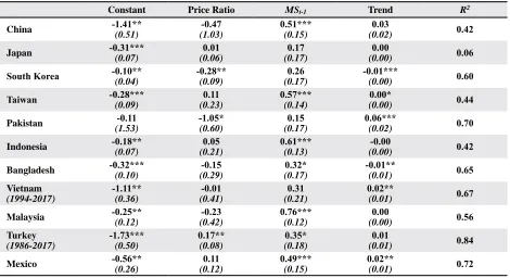
RESULTS

The Armington model was estimated using SAS 9.3 (SAS Institute, Cary NC). Estimation results obtained from the U.S. cotton market share equation in major cotton importing countries are reported in Table 2. All equations were estimated in log linear form and hence the elasticity estimates can be read

(6)

Table 1. Summary Statistic for Model Variables

Mean Standard Deviation Minimum Maximum

Market Share (%)

Bangladesh 0.17 0.13 0.03 0.56

China 0.06 0.05 0.00 0.19

Indonesia 0.36 0.13 0.12 0.64

Japan 0.48 0.12 0.21 0.81

Malaysia 0.27 0.23 0.04 0.75

Mexico 0.46 0.30 0.00 0.88

Pakistan 0.02 0.02 0.00 0.06

South Korea 0.53 0.22 0.15 0.97

Taiwan 0.38 0.15 0.11 0.74

Turkey (1986-2017) 0.17 0.13 0.01 0.43

Vietnam (1994-2017) 0.26 0.13 0.04 0.46

Price Ratio

Bangladesh 1.02 0.30 0.58 1.85

China 1.12 0.49 0.35 2.15

Indonesia 1.04 0.27 0.64 1.87

Japan 1.05 0.27 0.64 1.89

Malaysia 1.09 0.28 0.67 2.05

Mexico 0.33 0.45 0.01 2.04

Pakistan 0.69 0.34 0.23 1.58

South Korea 0.71 0.29 0.17 1.11

Taiwan 1.20 0.32 0.76 1.92

Turkey (1986-2017) 1.10 0.27 0.76 1.93

Vietnam (1994-2017) 1.06 0.27 0.75 1.93

Table 2. U.S. Cotton Market Shares in Major Importing Countries, 1978-2017

Constant Price Ratio MSt-1 Trend R2

China -1.41**

(0.51) (1.03)-0.47 0.51***(0.15) (0.02)0.03 0.42

Japan -0.31***

(0.07)

0.01

(0.06)

0.17

(0.17)

0.00

(0.00) 0.06

South Korea -0.10**_(0.04) -0.28**_(0.09) _(0.17)0.26 -0.01***_(0.00) 0.60

Taiwan -0.28***_(0.09) _(0.23)0.11 0.57***_(0.14) _(0.00)0.00* 0.44

Pakistan -0.11

(1.53) -1.05*(0.60) (0.17)0.15 0.06***(0.02) 0.70

Indonesia -0.18**

(0.07) (0.21)0.05 0.61***(0.13) (0.00)-0.00 0.42

Bangladesh -0.32***

(0.10)

-0.15

(0.29)

0.32*

(0.17)

-0.01**

(0.01) 0.65

Vietnam

(1994-2017) -1.11**(0.36) (0.41)-0.01 (0.21)0.31 0.02**(0.01) 0.67

Malaysia -0.25**

(0.12) (0.42)-0.23 0.76***(0.12) (0.00)0.00 0.56

Turkey

(1986-2017) -1.73***(0.50) 0.17**(0.08) (0.18)0.35* (0.01)0.01 0.84

Mexico -0.56**

(0.26) (0.12)0.11 0.49***(0.15) 0.02**(0.01) 0.72

(7)

The elasticity of U.S. cotton import share with respect to the price ratio (also referred to as the

substitution elasticity, σ) provides an indication

of the degree of sensitivity of U.S. cotton share in foreign markets and the magnitude of competition between U.S. cotton and cotton from other sources

in importing countries. A relatively high coefficient,

in absolute terms, indicates a high degree of com-petition between the U.S. and other cotton exporters. The short-run substitution elasticity ranges from -0.01 (Vietnam) to -1.05 (Pakistan). That is to say, U.S. cotton shows a high degree of competition with other cotton exporting countries in Pakistan (-1.05), followed by South Korea (-0.28) and the least com-petition in importing countries of Vietnam (-0.01) and Japan (0.01). Most substitution elasticities are estimated to be negatively related to the U.S. cotton market shares as expected. However, for Japan, Tai-wan, Indonesia, Turkey, and Mexico, the estimates are positive. A possible explanation is that the import demands for U.S. cotton from these countries are relatively small compared to other major importers.

Thus, the influence of the changes in the price ratio is not significant on the market shares.

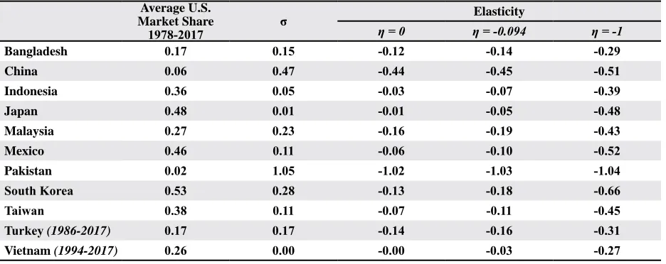
The overall elasticities of demand for U.S. cotton (

η

) are summarized in Table 3. These elasticity esti-mates were calculated based on certain assumptions about

η

. Specifically, an upper bound of 0 (perfectly inelastic) and a lower bound of -1 (unitary elasticity) were assumed. Additionally, a third estimate was calculated using an empirical estimate of -0.09 as the total demand elasticity. (The estimate of total demand elasticity of U.S. cotton is obtained from the Global Fibers Model developed at the Interna-tional Center for Agricultural Competitiveness at

Texas Tech University [Pan and Hudson, 2011].) The results indicate that Ni US is in the inelastic range

for all countries, except for Pakistan. The short-run demand elasticity for U.S. cotton ranged from -0.03 to -1.03 (

η

= -0.09). With other conditions remaining constant, a 1% increase in the relative price ratio would result in a 1.03% fall in the U.S. cotton export demand in Pakistan, but only a 0.03% fall in the U.S. cotton export demand for Vietnam. The lower export demand elasticities (in absolute terms) for Indonesia, Japan, Mexico, South Korea, Taiwan, and Vietnam could be explained by the relatively large U.S. cotton market shares for these countries. Being the largest cotton importer and an important destination market for exporting countries, the demand elasticity for U.S. cotton in China was estimated to be -0.45 (

η

= -0.09). This result is close to findings in Muham -mad et al. (2012), who reported that the conditional demand elasticity for China’s cotton imports was -0.63 during 2005 to 2010.

In addition, the findings indicate that the demand elasticity for U.S. cotton exports (Nus)

changes, sometime substantially, under alternative assumptions about

η

in all foreign markets, except for China and Pakistan. For example, the elasticity of demand for South Korea increases from -0.13 to -0.66 as

η

changes from 0 to -1. This result suggests that the import demand of U.S. cotton in South Ko-rea is sensitive to the overall elasticity of demand for all cotton in that region. On the other hand, China and Pakistan do not appear to be sensitive to changes in

η

, which suggests that U.S. cotton acts as a substitute for cotton from other regions, such as Australia, India, and Uzbekistan, mainly due to the geographic proximity.

Table 3. Calculation of Export Demand Elasticities for U.S. Cotton (1978-2017) Average U.S.

Market Share

1978-2017 σ

Elasticity

η = 0 η = -0.094 η = -1

Bangladesh 0.17 0.15 -0.12 -0.14 -0.29

China 0.06 0.47 -0.44 -0.45 -0.51

Indonesia 0.36 0.05 -0.03 -0.07 -0.39

Japan 0.48 0.01 -0.01 -0.05 -0.48

Malaysia 0.27 0.23 -0.16 -0.19 -0.43

Mexico 0.46 0.11 -0.06 -0.10 -0.52

Pakistan 0.02 1.05 -1.02 -1.03 -1.04

South Korea 0.53 0.28 -0.13 -0.18 -0.66

Taiwan 0.38 0.11 -0.07 -0.11 -0.45

Turkey (1986-2017) 0.17 0.17 -0.14 -0.16 -0.31

(8)

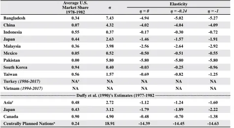
DISCUSSION

To a limited extent, our model results can be

compared to results obtained by Duffy et al. (1990).

To that end, our model was used to calculate U.S. cot-ton export demand elasticities during 1978 to 1982 to facilitate comparison with the previous work by

Duffy et al. (1990). It is worth noting that Duffy et al.

(1990) estimated the elasticities over the period from 1977 to 1982. However, due to the data availability,

the time period of 1978 to 1982 was analyzed in our

study. In addition, following Duffy et al. (1990), an

empirical estimate of -0.24 was assumed for the total elasticities of demand for cotton (

η

). The resulting comparison is presented in Table 4.

Due to the differences in the definition of regions

and time periods of analysis, U.S. cotton export elasticities can be compared only on a limited ba-sis (bottom of Table 4). Estimates for Japan (-1.46 to -1.91) are reasonably close to those obtained by

Duffy et al. (-1.79 to -2.22). In addition, estimates for China are comparable with Duffy et al. (1990).

However, it is important to note that their estimates were based on Centrally Planned Nations including the USSR and Eastern Europe, whereas the current estimates for China were based on mainland China

and Hong Kong. The import demand for U.S. cot-ton in this region ranged from -14.39 to -14.63 as

η

changed from 0 to -1 as estimated by Duffy et al. (1990). Consistent with the previous finding by Duffy

et al. (1990), our estimates remained elastic (from -4.02 to -4.09) under alternative assumptions about

η

. However, the magnitudes are significantly higher in Duffy et al.’s (1990) results due to the difference in region definition. Overall, the estimates presented here are well within the range reported by Duffy et al.

(1990), who used the similar Armington framework for estimation.

Kalman Filter Estimates of the Demand Models. Equations 8 and 9 were estimated using EViews 10 (IHS Global Inc., Irvine, CA), and the results are presented in Table 5. (Note: the TVP pro-cedure in EViews does not calculate the

goodness-of-fit measure [R2_{] and other diagnostic statistics} because the specification of the TVP model is free

from the usual assumptions made in the traditional regression model about the residual term.) Because the transition equations all follow a random walk process, they are omitted from the table. The estimates of the demand elasticities reported in

Table 5 are the final state demand elasticities (i.e.,

December, 2017).

Table 4. Comparison of Export Demand Elasticities for U.S. Cotton Average U.S.

Market Share

1978-1982 σ

Elasticity

η = 0 η = -0.24 η = -1

Bangladesh 0.34 7.43 -4.94 -5.02 -5.27

China 0.07 4.32 -4.02 -4.04 -4.09

Indonesia 0.55 0.37 -0.17 -0.30 -0.72

Japan 0.44 2.63 -1.46 -1.57 -1.91

Malaysia 0.36 3.98 -2.56 -2.64 -2.92

Mexico 0.05 0.52 -0.50 -0.51 -0.55

Pakistan 0.00 5.80 -5.80 -5.80 -5.80

South Korea 0.94 0.40 -0.03 -0.25 -0.96

Taiwan 0.56 1.57 -0.69 -0.82 -1.25

Turkey (1986-2017) NAz _NA _NA _NA _NA

Vietnam (1994-2017) NA NA NA NA NA

Duffy et al. (1990)’s Estimates (1977-1982

Asiay 0.48 2.72 _-1.12 -1.24 -1.60

Japan 0.43 3.12 -1.79 -1.89 -2.22

Canada 0.90 4.90 -0.48 -0.70 -1.38

Centrally Planned Nationsx 0.24 _18.91 -14.39 -14.45 -14.63

z NA denotes unavailable.

y Japan, Hong Kong, Philippines, Thailand, Malaysia, Republic of China, and Indonesia.

(9)

Based on the estimation results, all income elastici-ties (lnYit) are significantly different from zero at the

1% significance level for major importing countries

listed Table 5. However, Japan and South Korea are

estimated to have negative and significant income elasticities. These results reflect that imported cotton

is considered an intermediate product used mainly as a raw material in textiles production, one of the major export commodities in these countries. In addition,

decreases in consumption of cotton fiber have been

particularly dramatic in Japan, followed by South Korea over the past few decades (Fig. 3). The price elasticities of demand for U.S. cotton (lnPit) are sig-nificant and exhibit the expected signs for all countries,

except for Japan, which is negative, but not statistically

significant. One possible explanation for the lack of statistical significance of the price elasticity in Japan is

that due to the rapid decline in consumption level it is not responsive to price changes. Price elasticities range from -0.13 (Indonesia) to -0.87 (Vietnam) (Table 5). All countries have price-inelastic demand for U.S. cotton. For example, China’s price elasticity of demand for U.S. cotton is -0.17, which means a 1% increase in cotton import price is associated with a 0.17% fall in U.S. cot-ton import demand. This result stands in contrast to the Armington result for China. But recall, this is end-state

(Dec. 2017) elasticities and there have been substantial changes in cotton markets, especially in China.

Figure 3. Domestic Cotton Consumption in Japan and South Korea, 1990 to 2017.

0 500 1,000 1,500 2,000 2,500 3,000

3,500 thousand bales

Japan South Korea

Table 5. Kalman Filter Estimates of the U.S. Cotton Export Demand Models

Intercept lnYit lnPit LL AIC SC

Bangladesh 0.14

(0.40) 1.41***(7.17) -0.31***(-6.31) -197.44 0.92 0.94

China 0.15

(0.34) 1.00***(3.41) (-1.74)-0.17* -213.62 1.07 1.09

Indonesia 0.10

(0.54) 0.81***(8.65) -0.13***(-4.17) 124.50 -0.51 -0.49

Japan -0.05

(-0.28) -3.68***(-8.72) (-0.87)-0.02 96.92 -0.40 -0.38

Malaysia 0.42

(1.11)

0.52***

(2.65)

-0.26***

(-3.17) -231.38 1.00 1.02

Mexico -0.27

(-0.82) 1.87***(11.03) -0.67***(-9.66) -148.98 0.64 0.66

Pakistan 0.36

(0.84) 2.97***(8.86) -0.82***(-9.21) -244.51 1.24 1.26

South Korea _(1.33)0.22 -0.90***_(-8.42) -0.21***_(-66.72) 167.17 -0.69 -0.67

Taiwan _(0.35)0.08 0.57***_(3.45) -0.16**_(-1.95) -13.11 0.08 0.10

Turkey (1986-2017) _(-0.32)-0.12 1.21***_(15.58) -0.35***_(-11.69) -179.91 1.01 1.04

Vietnam (1994-2017) _(0.47)0.14 3.12***_(16.80) -0.87***_(-15.30) -87.49 0.66 0.69

Note: The values in parentheses are the z-statistics. LL is the value of the log likelihood, and AIC and SC are the Akaike information criterion and the Schwarz criterion, respectively. Different specifications of the TVP model for each origin country were tried, and the models with the smallest AIC and SC are presented here.

* denotes significance at 10%, **denotes significance at 5%, ***denotes significance at 1%.

Time-Varying Demand Elasticities. Although demand elasticities in the recent period are important, one of the objectives of this paper is to examine the evolution of the U.S. cotton export demand elasticities

over time. Figure 4 illustrates the Kalman filter esti -mates of the evolving price elasticities for U.S. cotton in major importing countries from 1978 to 2017. The initial state of this model is calculated with likelihood

(10)

the initialization, the Kalman filter estimates can be

obtained by recursive calculation of state vector. China consistently has been the world’s largest importer since 2003, and the U.S. is the largest sup-plier to Chinese cotton imports. As shown in Fig. 4,

there are bigger fluctuations in the China model in

early years and imports remained relatively constant in later part of the period from 1995 to 2017

(ap-proximately -0.2). This could be reflecting the trade liberalization efforts that have been taking place in

China in recent years. In the early 1980s, China’s

trade position was highly volatile, changing from the world’s largest importer to the world’s largest exporter. Since the late 1990s, driven by its rapid expansion of textile manufacturing and trade liberalization, particularly the phasing out of the MFA between 1995 and 2005 and its entry into the WTO in 2001,

China’s import demand elasticity for cotton became stable and less elastic. Through political changes and structural reforms, China is becoming more stable, and perhaps economically rational, in its response to market price signals.

-4 -3 -2 -1 0 1 2 3 4

1980 1985 1990 1995 2000 2005 2010 2015 Price elasticity ± 2 RMSE

Bangladesh

-4 -3 -2 -1 0 1 2 3 4

China

-4 -3 -2 -1 0 1 2 3 4

Malaysia

-2.0 -1.5 -1.0 -0.5 0.0 0.5 1.0 1.5 2.0

Japan

-4 -3 -2 -1 0 1 2 3 4

Indonesia

-1.5 -1.0 -0.5 0.0 0.5 1.0 1.5 2.0 2.5

(11)

Over time, a stable and slightly increasing de-mand elasticity for U.S. cotton imports is observed for Asian countries during the study period, including Indonesia, Japan, Malaysia, South Korea, and Taiwan. Most apparent is a general trend of inelasticity over this period. These countries have either maintained or moderately increased total cotton consumption over the past two decades. Given their commercial ties and long-time market presence, U.S. cotton is

seen more as a necessity in these markets. On the other hand, the stronger market position of U.S. cotton in these markets could be partially explained by the perceptions of high quality and information services of U.S. cotton. Thus, the import elasticities maintained the trend to the end of the period.

Although most countries have moderate increases in consumption, increases have been large in Viet-nam and Bangladesh, with less dramatic increases in

Figure 4. Kalman Filter Estimates of Price Elasticities for Selected Countries.

-4 -3 -2 -1 0 1 2 3 4

Pakistan

-2.0 -1.5 -1.0 -0.5 0.0 0.5 1.0 1.5 2.0

South Korea

-4 -3 -2 -1 0 1 2 3 4

84 86 88 90 92 94 96 98 00 02 04 06 08 10 12 14 16 Price elasticity ± 2 RMSE

Taiwan

-4 -3 -2 -1 0 1 2 3 4

88 90 92 94 96 98 00 02 04 06 08 10 12 14 16 Price elasticity ± 2 RMSE

Turkey

-4 -3 -2 -1 0 1 2 3 4

94 96 98 00 02 04 06 08 10 12 14 16 Price elasticity ± 2 RMSE

(12)

Pakistan and Turkey. Vietnam and Bangladesh have emerged recently as important cotton importers to supply newly developed textile industries. The general movement to less elastic demand elasticities suggests strong trade ties with these countries. Although U.S.

cotton suffers a disadvantage in terms of transporta -tion costs in comparison to cotton exports from other countries, such as Australia and India, the high, and reliably known, quality of U.S. cotton are favored by importers, suggesting these countries become less price responsive to U.S. cotton imports over time.

In Mexico, a sharp decline in import demand elasticity for U.S. cotton is observed during 1978 to 1983. In the latter part of the study period, the import demand elasticity increased slightly and remained inelastic over time. This can be explained by the geo-graphic proximity to the U.S., which makes the U.S. the consistent supplier of cotton for Mexico. More importantly, the implementation of NAFTA in 1995 led to large quantities of cotton delivered to Mexico as trade relationship was established. As a result, the price elasticity became more inelastic in recent years. A broader look at the results suggests a general trend towards less elastic demand from the beginning compared to the end of the period, which implies that importers have become less sensitive to changes in U.S. cotton prices. In particular, the graphs demonstrate stable movements since the late 1990s,

mainly a reflection of the impacts of stronger trade

relationships established to lower trade barriers in the world cotton market. In particular, the formation

of the WTO has a more direct influence on agricul -tural goods, including cotton, which allowed more

vibrant trade flows and fostered more integration

of economies. Moreover, the elimination of MFA between 1995 and 2005 and the full liberalization in international textile and apparel markets encouraged textile production in developing countries,

particu-larly in Asia, which significantly stimulated cotton

demand from the U.S. Another factor that could contribute to the inelastic import elasticity is that U.S. cotton is perceived to be better quality than that of other suppliers. Therefore, U.S. cotton competes

effectively with cotton imports from other regions.

CONCLUSIONS

As U.S. cotton exports account for a large share of total U.S. production, a knowledge of relevant elasticities has become more important in determin-ing the domestic price, farm income, and government

costs in designing appropriate agricultural policy. Given the important changes in agricultural and trade policies that occurred in the last two decades have

affected the world cotton market considerably, these

elasticities need to be reexamined and updated. This study provides new estimates of the foreign export demand elasticity for U.S. cotton using an Armington framework for 1978 to 2017. Based on the estima-tion results, the short-run price elasticities of foreign demand for U.S. cotton are price inelastic for major cotton importing countries, except for Pakistan. Price elasticities for demand of U.S. cotton in these coun-tries ranged from -0.03 to -1.03, if -0.09 was assumed for the overall elasticities of demand for U.S. cotton (

η

). Variations in the elasticities’ estimates are mainly

attributed to differences in U.S. cotton market shares in different U.S. cotton importing countries/regions.

Countries with lower export demand elasticities (in absolute terms) are associated with relatively large U.S. cotton market shares for these countries.

Another objective of this study is to empirically examine the foreign demands of U.S. cotton exports in a dynamic framework of TVP. For this purpose, the

Kalman filter approach within a state-space model is

utilized in the estimation using monthly data during 1978 to 2017. This approach is well suited to simulate the structural change of demand models that have been altered by unobservable factors such as consumer taste, expectations, and policy and regime changes. Global consumption of cotton by textile mills has increased dramatically in recent years. Rapid growth corresponded with trade liberalization, particularly the phase-out of the MFA, and mill use has shifted toward developing countries in Asia, particularly in China. Other newly emerging textile producers (and hence major cotton consumers) are Bangladesh and Vietnam. Our results indicate that the overall trend for U.S. cotton in the most recent years is that the import demand elasticity seems to be becoming less elastic, implying that cotton import demand has become less price sensitive than it was historically in these import-ing countries. Because of strong trade relationships, long time market presence, better quality and informa-tion services of U.S. cotton, the U.S. has competitive advantages in these major cotton importing countries over other suppliers.

ACKNOWLEDGMENTS

(13)

REFERENCES

Armington, P.S. 1969. A theory of demand for products distin-guished by place of production. IMF Staff Papers 16, no. 1:159–178.

Babula, R.A. 1987. An Armington Model of U.S. cotton exports. J Agric. Econ. Res. 39(4):12–22.

Cooley, T.F., and E.C. Prescott. 1976. Estimation in the pres-ence of stochastic parameter variation. Econometrica: J. Econometric Soc. 167–184.

Devadoss, S., and W.H. Meyers. 1990. Variability in wheat export demand elasticity: policy implications. Agric. Econ. 4(3-4):381–394.

Duffy, P.A., M.K. Wohlgenant, and J.W. Richardson. 1990. The elasticity of export demand for US cotton. Amer. J. Agric. Econ. 72(2):468–474.

Durbin, J., and S. J. Koopman. 2012. Time Series Analysis by State Space Methods. Vol. 38. Oxford University Press, Oxford, U.K.

Feenstra, R.C., P. Luck, M. Obstfeld, and K.N. Russ. 2014. In search of the Armington elasticity. No. w20063. National Bureau of Economic Research, Washington, D.C.

Gardiner, W., and P.M. Dixit. 1987. Price elasticity of export demand: concepts and estimates. Foreign Agricultural Economic Report (USA). U.S. Dept. of Agriculture, Economic Research Service, Washington, D.C.

Harvey, A.C. 1990. Forecasting, Structural Time Series Mod-els and the Kalman Filter. Cambridge University Press, Cambridge, U.K.

Kalman, R.E. 1960. A new approach to linear filtering and prediction problems. J. Basic Eng. 82(1):35–45.

Kim, C.-J., and C.R. Nelson. 1999. State Space Models with Regime Switching. MIT Press Books, Cambridge, MA.

Miller, D.J., and P.L. Paarlberg. 2001. An Alternative Ap-proach To Determining The Elasticity Of Excess De-mand Facing The United States.” 2001 Annual meeting, August 5-8, Chicago, IL 20587, American Agricultural Economics Association (New Name 2008: Agricultural and Applied Economics Association).DOI: 10.22004/ ag.econ.20587

Muhammad, A., L. McPhail, and J. Kiawu. 2012. Do US cotton subsidies affect competing exporters? An analy-sis of import demand in China. J. Agric. Appl. Econ. 44(2):235–249.

Nerlove, M. 1958. Distributed Lags and Demand Analysis. Agriculture Handbook No.141. U.S. Department of

Agri-culture, Washington D.C.

Pan, S., and D. Hudson. 2011. Technical Documentation of the World Fiber Model. International Center for Agricultural Competitiveness, Department of Agricultural and Applied Economics, Texas Tech University, Lubbock, TX.

Reimer, J.J., X. Zheng, and M.J. Gehlhar. 2012. Export de-mand elasticity estimation for major US crops. J. Agric. Appl. Econ. 44(4):501–515.

Sarris, A.H. 1983. European community enlargement and world trade in fruits and vegetables. Amer. J. Agric. Econ. 65(2):235–246.

Slade, M.E. 1989. Modelling stochastic and cyclical compo-nents of technical change: an application of the Kalman filter. J. Econometrics. 41(3):363–383.

United States Department of Agriculture. Foreign Agricul-tural Service. Global AgriculAgricul-tural Trade System [USDA GATS]. 2018. Data available online at https://apps.fas. usda.gov/gats (verified 23 Oct. 2019).

United States Department of Agriculture. Foreign Agricultural Service. Production, Supply and Distribution [USDA PSD]. 2018. Data available online at https://apps.fas.

usda.gov/psdonline/app/index.html#/app/advQuery

(verified 23 Oct 2019).