DESERT 17 (2012) 41-48
Flood Flow Frequency Model Selection Using L-moment Method
in Arid and Semi Arid Regions of Iran
A.R. Keshtkar
a*, A. Salajegheh
b, M. Najafi Hajivar
ca Assistant Professor, International Desert Research Center (IDRC), University of Tehran, Tehran, Iran b Associate Professor, Faculty of Natural Resources, University of Tehran, Karaj, Iran c MSc. Graduate, Natural Resources and Watershed Management Office, Koohrang, Iran
Received: 3 November 2009; Received in revised form: 2 March 2012; Accepted: 4 April 2012
Abstract
Statistical frequency analysis is the most common procedure for the analysis of flood data at a gauged location that in first step it is needed to select a model to represent the population. Among them, the central moment has been the most common and widely used, and with the using of computers, the application of the maximum likelihood has increased. This research was carried out in order to recognition of suitable probability distributions with pervious common methods. In order to investigate of suitable probability distribution for flood flow, using L-moment method through the existing hydrometric stations in the region, 17 hydrometric stations were selected for peak discharges data studies. According to results of this research for peak discharge, LP3 distribution and ordinary moment method, P3 distribution and L-moment method, LN2 and LN3 distributions and ordinary method have been suitable distinguished for 53%, 35%, 6% and 6% of stations, respectively. We concluded that L-moment method is suitable to determine peak series probability distributions in the Iran central plateau and P3 is the best probability distribution for modeling peak series in this region.
Keywords: Flood flow; Frequency distribution function; Linear moment; Maximum likelihood; Ordinary moment
1. Introduction
Hydrological frequency analysis is one of the essential tasks in hydrological engineering design. It is the work of determining the magnitude of hydrological variables corresponding to given frequencies or recurrence intervals (McCuen, 2003). Procedures involved in frequency analysis include: collection a random sample of the interested hydrological variables; finding the best-fit-distribution for the samples by a good-of-fit (GOF) test or other appropriate methods; and determining the magnitude of the hydrological variable corresponding to a given probability of exceedance using the best-fit-distribution. Chow (1951) proposed the following general equation for hydrologic frequency analysis of a random variable X with
Corresponding author. Tel.: +98 21 88971717, Fax: +98 21 88971717.
E-mail address:[email protected]
mean μ and standard deviation σ:
XT = μ + KT σ (1)
Where KT, the frequency factor is a function of the return period T and is dependent on the distribution type of X. Frequency factors of distributions commonly used in hydrologic frequency analysis are themselves variables and their distributions have been identified (Kite, 1988). Upon collection of a random sample, one must decide the type of distribution which best characterizes the random sample and determine the corresponding KT value.
Two GOF tests, namely the chi-square test and the Kolmogorov-Smirnov test, are often used for the selection of probability distributions for hydrological variables (Haan, 2002). Another method of goodness-of-fit test is the method based on ordinary moment ratio diagrams (D, Agostino and Stephen, 1986).
been many applications of L-moments diagrams for selecting various distributional alternatives in a region and the skewness and kurtosis L-moment-ratio diagram (LMRD) was suggested as a useful tool for discrimination between candidate distributions (Hosking and Wallis, 1987; Hosking, 1990; Hosking and Wallis, 1993; Vogel and Fennesset, 1993; Hosking and Wallis, 1997 and Peel et al., 2001). The L-moments uniquely define the distribution if the mean of distribution exists, and the L-skewness and L-kurtosis are much less biased than the ordinary skewness and kurtosis (Hosking and Wallis, 1997).
Estimation of flood flow is often required for watersheds with insufficient or nonexistent hydrometric information particularly in arid and semi-arid regions. Because parametric methods require a number of assumptions, nonparametric methods have been investigated as alternative methods. L-moment diagrams and associated goodness-of-fit procedure (Wallis, 1988; Hosking, 1990; Chowdhury et al., 1991; Pearson, 1992; Vogel et al., 1993a; Daviau et al., 2000; Peel et al., 2004; Yurekli et al., 2005; Chen et al., 2006; Eslamian and Feizi, 2007 and Salajegheh et al., 2008) have been advocated for evaluating the suitability of selecting various distributional alternatives for modeling flows in a region. For example Wallis (1988) found an L-moment diagram useful for rejecting Jain and Singh’s (1987) conclusion that annual maximum flood flows at 44 sites were well approximated by a Gumbel distribution and for suggesting a general extreme value (GEV) distribution instead. Vogel et al., (1993b) used L-moment diagrams to show that two and three-parameter log-normal models (LN2 and LN3),
(2001) used L-moment diagrams to show that the Gumbel distribution was acceptable for annual maximum series (AMS) in the north of Iran.
Base on the climate conditions and annual average precipitation, Iran is one of the arid and semi-arid countries of the world, which is mostly encountered with lack of water. Most of the rivers in arid regions of Iran are seasonal and their flood flows may become unavailable during a short time of rainfall seasons and because of some special geological problems of this region most of the permanent rivers contain saline water and are useless. The objective of the present study is to introduce and evaluate the suitable probability distributions for modeling peak flows in arid and semi-arid regions of Iran.
2. Materials and Methods
2.1. Study area
The Iran central plateau watershed where is located in center of Iran, has considered as a arid and semi-arid region of Iran. The Iran central plateau watershed is 854000 Km2 in area
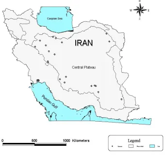
and has seven sub watersheds and several catchments in different size. For the purpose of this research 17 catchments were chosen where permanent river and hydrometric station had. The selection was based on Ministry of Agriculture information that no significant abstraction exist in the contributing catchments upstream of these stations. The location of the hydrometric stations utilized in this research is given in table 1 and the spatial distribution shown in fig.1.
Table 1. Main characteristics of stations under investigation and data series analyzed
Station River Longitude (E) Latitude (N) Altitude (m) Catchment area (Km2)
Sarab hendeh Golpaiegan 50 33 21 2000 817
Abgarm Kharood 48 18 33 45 1560 2450
Dehsomee Kordan 50 50 35 57 1410 360
Sira Karaj 51 09 36 02 1790 725
Dodahak Ghomrood 50 34 34 28 1470 8851
Chamriz Kor 52 07 30 28 1800 3390
Baft Soltani 56 32 29 05 2000 935
Safarzadeh Halilrood 57 33 28 52 920 8420
Dehrood Shoor 57 44 28 52 1000 1321
Adoori Talango 58 07 28 58 1690 276
Jirofto Haftkoosk 57 11 29 34 2600 225
Ghariatolarab Chary 56 02 29 37 1853 173
Godarzarch Abbakhsha 56 34 29 34 2200 1144
Namrood Namrood 52 39 35 43 1810 587
Simindasht Delichai 52 31 35 31 1435 2254
Bonkooh Hablerood 52 52 35 18 1000 3209
Fig. 1. Location of the study area
2.2. Methods
In this research, several methods were carried out in order to propose the most suitable probability distributions for peak series. From the hydrometric stations existing in the watershed, 17 stations were selected for analysis. The peak flows data were available for 17 gauging stations, with stream flow records of 20 years or more. Most of the data were recorded between 1972 and 2000.
Then, data were analyzed to choose an identical data period. Therefore, the peak series data from 1971 to 1998 were taken as the 25-year data period of each station.
The missing data were generated and completed using regression relationships between the stations. For each distribution, the values of residual sum of squares (RSS) were calculated using the ordinary moment and L-moment methods. The RSS values of the two methods were compared, suitable distributions for each station were chosen according to the lowest RSS. The best of probability distribution was applied to estimate T-year peak series.
2.3. The ordinary moment ratio diagram
Parameters of a probability distribution can be expressed in terms of its moments (μ'r) or
central moments (μr) defined as
μ'r = E (X') (2a)
μr = E (X – μ1r)r (2b)
For r= 1, 2 therefore, the shape of a probability distribution can be characterized by the moments of that distribution. This is achieved using the relationships between the standardized coefficients of skewness ( ) and kurtosis (β2)
which are defined as
= μ3/(μ2)3/2 (3a)
β2 = μ4/(μ2)2 (3b)
Theoretical β2 relationships of various
sample estimates of and β2 are defiened as
(4a)
b2 = (4b)
Where
mr = (4c)
S= (4d)
Sample estimates of ) and (β2) do
not always coincide with the theoretical points or curves of their parent distributions, and method of GOF test using ( b2) have thus
been developed for normal distribution (D,Agostino and Pearson, 1973 and Bowman
and Shenton, 1975). Bowman and Shenton (1986) developed acceptance regions for a , β2) based GOF test using stochastic
simulation. The sample moments ( b2) tend
to have high variances, especially when the sample size is small. Therefore, it is often difficult to distinguish among candidate distributions. Even though the joint distribution of the ordinary sample skewness and sample kurtosis is sympototically normal, such asympototic property is a poor approximation in small and moderately samples, particularly when the underlying distribution is even moderately skew (Hosking and Wallis, 1997). Using stochastic simulation, Wu (2005) studied the distribution of ( b2) for normal
distribution with respect to sample sizes varying from 20 to 1000. As can be seen in fig. 2, for smaller sample sizes (for example n=20) the distribution of given b2 changes from
unimodality to bimodality as b2 increases. Thus,
closed curves encompassing certain percentages of ( b2) samples of the normal distribution
are difficult to be expressed by mathematical equations when the sample size is small.
L-moment analysis
L-moment is alternative system of describing the shapes of probability distributions. L-moments are linear combinations of order statistics which are robust to outliers and virtually unbiased for small samples, making
Hosking and Wallis, 1993). L-moments are defined as linear combinations of probability weighted moments (PWM):
βr =E{X[Fx(x)r]} (5)
Where βr is the rth order PWM and Fx(x) is the
cdf of X. When r=0, β0 is the mean stream flow.
Hence a sample estimate of the first PWM, which we term b0 is simply the sample mean. Nevertheless, unbiased estimators are often preferred in goodness-of-fit evaluations such as L-moment diagrams. Unbiased sample estimates of the PWMs, for any distribution can be
computed from
b = (6a)
b1= (6b)
b2 = (6c)
b3= (6d)
Where xj represents the ordered stream flows
with x1 being the largest observation and xn the
smallest. The PWM estimators in eqn. (6) can be more generally described using
br = (7)
For a random variable X with quantile function
x (u), Hosking and Wallis (1997) defined the
L-moments (λr, r = 1,2, …) as
λr= (8a)
Where
, r=0,1,2,… (8b)
(8c)
Greenwood et al., (1979), and for any distribution, the first four L-moments are easily computed from PWMs using
λ1=β0 (9a)
λ2 =2β1 - β0 (9b)
λ3 =6β2 - 6β1- β0 (9c)
λ4 =30β2 - 12β1- β0 (9d)
Where βr, r = 0,1,2,…, are probability weighted
moments defined by
βr= (10)
In terms of linear combination of order statistics, the L-moments can also be expressed by
λ1 = (11a)
λ2 = (11b)
λ3 = (11c)
λ4 = (11d)
Where Xk:n is the K-th order statistic from a
random sample of size n. similar to the ordinary moment ratios, the L-moment ratios are defined by
(12)
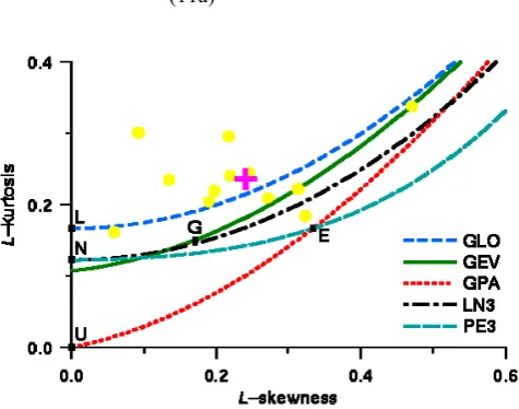
Theoretical relationships between L-skewness (τ3) and L-kurtosis (τ4), i.e. the L-moment ratio
diagram of several probability distributions have been given by Hosking (1990 and 1991) and can be used to distinguish different probability distributions.
Fig. 2. L-moment ratio diagram of various distributions
L-moment ratio diagrams
Analogous to the product moment ratio; coefficient of variation Cv = σ / μ, skewness γ
and kurtosis k, Hosking (1990) define the
L-moment ratios
(13a)
(13b)
(13c)
Where λ, r = 1, …, 4 are the first four L-moments and τ2, τ3 and τ4 are the L-coefficient
of variation (L-Cv), L-skewness and L-kurtosis,
respectively. The first L-moment λ1 is equal to
the mean stream flow μ; hence it is a measure of location. Hosking (1990) shows that λ2; τ3 and
τ4 can be thought of as measures of a
distribution’s scale, skewness and kurtosis, respectively, analogous to the moment's σ, γ and
discharge and based on computed residual sum of squares (RSS), LP3 distributions and ordinary moment method, P3 distribution and
L-6% of stations, respectively (Table 2). Estimated T-year peak series using the best of probability distribution have shown in table 3.
Table 2. Suitable probability distributions and methods for peak series
Station RSS
Suitable Probability Distribution Suitable Method Sarab hendeh 40 P3 L-moment Abgarm 15 LP3 Ordinary moment Dehsomee 5.9 LN3 Ordinary moment Sira 8.2 LP3 Ordinary moment Dodahak 18 LP3 Ordinary moment Chamriz 8.9 LP3 Ordinary moment Baft 16.9 LP3 Ordinary moment Safarzadeh 10.5 LP3 Ordinary moment Dehrood 9.4 LP3 Ordinary moment Adoori 34.4 P3 L-moment Jirofto 11.2 P3 L-moment Ghariatolarab 10.6 P3 L-moment Godarzarch 14.1 LP3 Ordinary moment Namrood 24.6 P3 L-moment Simindasht 22.8 P3 L-moment Bonkooh 12.1 LP3 Ordinary moment Senobar 15.3 LN2 Ordinary moment
Table 3. Estimated T-Year peak series
T-Years Station
2 5 10 20 50 100 Sarab hendeh 80 120 144 162 188 205 Abgarm 73 90 99 107 121 130 Dehsomee 57 77 89 101 116 128 Sira 87 120 142 159 192 214 Dodahak 62 84 99 111 132 147 Chamriz 341 398 433 457 500 527 Baft 47 82 108 144 171 238 Safarzadeh 273 403 496 571 719 821 Dehrood 275 339 379 408 460 495 Adoori 100 127 143 157 171 181 Jirofto 22 31 35 41 44 48 Ghariatolarab 16 17 18 19 20 20 Godarzarch 41 59 71 80 95 105 Namrood 30 51 60 68 77 84 Simindasht 39 52 60 66 74 78 Bonkooh 33 44 48 57 67 71 Senobar 97 140 169 198 237 266
For two methods sum of scores obtained in order to better comparison between distributions. First rank was gave to each distribution that RSS estimated was lowest and fifth rank for each distribution that RSS estimated was highest and in equal scores, ranking was similar. Finally sum of scores were computed for any distribution that according this method distribution was best that was accepted lowest score (Fig. 3).
4. Conclusion
The goal of this study was to select a set of suitable probability observed distributions for modeling peak series in arid and semi-arid
of peak series across the entire Iran central plateau, however, separation of central plateau in to broad homogeneous regions can improve our ability to discriminate among potential flood flow frequency models such that the P3 distribution provides the best approximation to the distribution of peak series in the most of this region. Of the models tested, the LP3, P3 and
LN2 distributions provides the best approximation to the distribution of peak series using ordinary moment method. Finally we concluded that L-moment method is suitable to determine peak series probability distributions in the Iran central plateau and P3 is the best probability distribution for modeling peak series in arid and semi-arid regions of Iran.
Fig. 3. Sum of scores obtained from peak series for different statistical distribution in L-moment and ordinary moment
References
Adamowski, K., 2000. Regional analysis of annual maximum and partial duration flood data by nonparametric and L-moment methods. Journal of Hydrology, 229: 219-231.
Bowman, K.O. and L.R. Shenton, 1975. Omnibus test contours for departures from normality based on and b2. Biometrika, 62: 243-250.
Bowman, K.O. and L.R. Shenton, 1986. Moment ( b2) techniques. In: D,Agostino, R.B. and M.A.
Stephen (Editors). Goodness-of-Fit Techniques. Marcel Dekker, New York.
Chen, Y.D., G. Huang, Q. Shao and C. Xu, 2006. Regional analysis of low flow using L-moments for Dongjiang basin, South China. Hydrological Science Journal, 51: 1051-1064.
Chow, V.T., 1951. A general formula for hydrologic frequency analysis. Transaction of American Geophysics Union, 32: 231-237.
Chowdhury, J.U., J.R. Stedinger and L. Lu, 1991. Goodness-of-fit tests for regional GEV flood distributions. Water Resource Research, 27: 1756- 1776.
D,Agostino, R.B. and E.S. Pearson,1973. Tests for
departure from normality. Emperical results for the distributions of b2 and Biometrika, 60: 613-622.
D,Agostino, R.B. and M.A. Stephen, 1986. Goodness-of-
Fit Techniques. Marcel Dekker, New York.
Daviau, J-L., K. Adamowski and G.G. Patry, 2000. Regional flood frequency anaysis using GIS, L- moment and geostatistical methods. Hydrological Processes, 14: 2731-2753.
Eslamian, S.S. and H. Feizi, 2007. Maximum monthly rainfall analysis using L-moments for an arid region in Isfahan province, Iran. Journal of Applied Meteorological and Climatology, 46: 494-503.
Gholami, A, 2001. To study of appropriate probability distributions for minimum, mean and maximum flows using L-moment method. Iranian Natural Resources Journal, 57: 115-127.
Greenwood, J.A., J.M. Landwehr, N.C. Matalas and J.R. Wallis, 1979. Probability weighted moments: definition and relation to parameters of several distributions expressible in invers form. Water Resource Research, 15: 1049-1054.
Haan, C.T., 2002. Statistical Methods in Hydrology. Ames, Iowa, Iowa state Press.
Hosking, J.R.M., 1990. L-moments: analysis and estimation od distributions using linear combinations of order statistics. J.R. Star. Soc., 52: 105-124. Hosking, J.R.M., 1991. Approximations for use in constructing L-moment ratio diagrams. Research Rep. RC-16635, IBM Research Division, T.J. Watson Research Center, Yorktown Hieghts, NY, 3p. Hosking, J.R.M. and J.R. wallis, 1987. Parameter and quantile estimation for the Generalized Pareto distribution. Technometrics, 29: 339-349.
Hosking, J.R.M. and J.R. Wallis, 1993. Some statistics useful in regional frequency analysis. Water Resource Research, 29: 271-281.
Hosking, J.R.M. and J.R. wallis, 1997. Regional frequency analysis: an approach based on L- moments. Cambridge University Press, Cambridge, UK.
Kite, G.W., 1988. Frequency and risk analysis in Hydrology. Water Resource Publication.
Kjeldson, T.R., J.C. Smithers and R.E. Schulze, 2002. Regional flood frequency analysis in the KwaZulu- Natal province, South Africa, using index-flood method. Journal of Hydrology, 255: 194-211.
kottegoda, N.T., 1980. Stochastic water resources technology. McMillan, London, UK.
October. Pp. 631-632.
Pearson, C.P. 1992. Frequency of high intensity rainfalls in Christchurch. Hydrology Centre Report CR92.11. Department of Scientific and Industrial Research, Christchurch, New Zealand. 55 p.
Peel, M.C., T.A. McMahon and B.L. Finlayson, 2004. Continental differences in the variability of annual runoff-update and reassessment. Journal of Hydrology, 295: 185-197.
Peel, M.C., Q.J. Wang and T.A. McMahon, 2001. The utility of L-moment ratio diagrams for selecting a regional probaility distribution. Hydrological sciences Journal, 46: 147-155.
Salajegheh, A., A.R. Keshtkar and S. Dalfardi, 2008. To study of the appropriate probability distributions for annual maximum series using L-moment method in arid and semi-arid regions of Iran. XIII World Water Congress, 1-4 september, Montpellier, France. Vogel, R.M. and N.M. Fennesset, 1993. L-moments
Jurnal of Hydrology, 146: 421-449.
Vogel, R.M., W.O. Thomas and T.A. McMahon, 1993b. Flood flow frequency model selection in Southwestern U.S.A. Journal of Water Resources Planning and management, ASCE, 119: 353-366. Vogel, R.M. and I. Wilson, 1996. Probability distribution of annual maximum, mean and minimum streamflows in the United States. Journal of Hydrologic Engineering, 1: 69-76.
Wallis, J.R., 1998. Catastrophes computing and containment: living in our restless habitat. Speculation Sci. Technology, 11: 294-315.
Wu, Y.C., 2005. Estabilishing acceptance regions for goodness-of-fit test by stochastic simulation. Master thesis, Department of Bioenivironmental Systems Engineering, National Taiwan University.