Desert
Online at http://desert.ut.ac.ir Desert 19-2 (2014) 99-109
Evaluating effect of downscaling methods; change-factor and
LARS-WG on surface runoff (A case study of Azam-Harat River
basin, Iran)
E. Goodarzi
a*, A.R. Massah Bavani
b, M.T. Dastorani
c, A. Talebi
aaDepartment of Watershed Management, Collage of Natural Resources, University of Yazd, Yazd, Iran bDepartment of Irrigation and Drainage Engineering, Collage of Abouraihan, University of Tehran, Pakdasht, Iran
cFaculty of Natural Resources and Environment, Ferdowsi University Of Mashhad (FUM), Mashhad, Iran Received: 3 November 2013; Received in revised form: 1 July 2014; Accepted: 29 September 2014
Abstract
This study aims to evaluate effects of two downscaling methods; change-factor and statistical downscaling on the runoff of the Azam-Harat River located at Yazd province (with an arid climate) of Iran, under the A2 emission scenario for the period of 2010-2039. For this purpose, CGCM3-AR4 model; a rainfall-runoff conceptual model, IHACRES; two downscaling models, Change Factor and LARS-WG were applied. Results show 30% difference in runoff simulated by two downscaling methods. Also, according to the fact that Change Factor ignores climate fluctuations over the course of future period relative to base period, simulated runoff from the outputs of this downscaling method does not contain enough confidence and cannot represent the actual runoff of the basin in the future. Despite, fluctuations are modeled in the LARS-WG well. On the other hand, if the estimated runoff increase from the LARS-WG is more than the capacity of the Azam-Harat River and Basin, the risk of flood and damage could figure in the future.
Keywords: Azam-Harat River Basin; Climate change; CGCM3-AR4; Downscaling; IHACRES; LARS-WG
1. Introduction
According to the last reports of the Intergovernmental Panel on Climate Change (IPCC), the surface of the Earth is warming and the climate is changing (IPCC, 2007). The recent observations of increases in global average temperatures, rising sea levels and melting ice and snow cover in the world confirm this theory. Global warming increases water vapour in the atmosphere, average rainfall, and the frequency of occurrence of maximum precipitation in dry areas (Dunn-Steel et al., 2008). In recent years, many studies on the impacts of climate change on hydrology and water resources in most regions of
Corresponding author. Tel.: +98 912 8468446, Fax: +98 21 88976173.
E-mail address:[email protected]
and Martinez, 2006). Simulation for the next 50 years by climate models has predicted a widespread drought in North America (Hughes & Diaz, 2008). Changes of climate variables of temperature and rainfall cause the occurrence of droughts, floods and other maximum events in arid areas that bring adverse effects on the lives of people living in these areas. According to previous research, the frequency of maximum climatic events such as floods and droughts is likely to increase with climate change (Tompkins, 2005). In addition, Mearns et al., (1996) found that climate change will increase the occurrence of the maximum events with spatial and temporal changes in climate fluctuations. Most of the predicted impacts of climate change on different systems for the future periods used output of general circulation models (GCMs).
However, one of the main problems of the outputs of the GCMs for impact assessment on a regional scale is the spatial and temporal course resolution of the calculation cell. Downscaling is the technique used for converting a coarse grid of GCMs to local and regional levels. Most studies all over the world use only one downscaling method, and many researchers apply the change factor (CF) for downscaling climatic variables (Reynard, 2001; Diaz-Nieto, 2005; Minville, 2008; and Tabor et al., 2010). They used the change factor for the purpose of downscaling climate variables. Massah Bavani et al., 2006 applied the CF method for downscaling GCMs to examine changes in temperature and precipitation on the inflow to the Chadegan dam. Their results showed a 5.8% reduction of inflow and three times increase of flow changes coefficient for the future periods. In other studies, climate change scenarios were produced by downscaling GCMs using statistical methods. Various statistical downscaling techniques have been developed to downscale course resolution outputs of GCMs to the finer scales (Kavli, 2003; Huth, 2005; Busuioc, 2008, etc.). In other research, artificial (stochastic) weather generator including WGN, CLIMGEN, CLIGEN and LARS-WG have been employed for downscaling outputs of GCMs (Babaeian et al., 2004; Dibike 2005; Semenov and Kilsby 2007; Abbasi et al., 2011). In this study, the LARS-WG model was used for the purpose of downscaling coarse resolution data of the study area. Since there are only few studies on this filed in the arid and semi-arid regions of Iran, this study tries to analyse the results of considering climate
fluctuations (using LARS-WG method) on the surface runoff of the regions, and the results of not considering these fluctuations (using the change factor method) in the modelling of future climate variables. In the CF method, fluctuations in climate variables are not considered, whilst LARS-WG model considers those volatility.
In this paper the studied behaviour of climate variables was studied in order to simulate the runoff of the Azam-Herat River Basin in southwest Yazd province under both downscaling approaches, CF and LARS-WG for the period of 2010 to 2039. In this regard, the GCM model, CGCM3-AR4 under the A2 emission scenario and a conceptual rainfall-runoff model (IHACRES) have been used.
2. Material and methods
2.1. Case study
Fig. 1. Geographical location of Azam-Herat Basin in Iran and distribution of the stations
2.2. Climatic dataset used in this study
The baseline data used in this study includes daily observation data of temperature, precipitation and runoff for the period of 1982 to 2008 from the selected stations in the study area. However, due to a lack of sufficient recorded data in the stations within the area, rain gauge and evaporation gauge data near the study area were used. After proving the accuracy and homogeneity of the data using a run-test method, the climate data of the stations near to the study area were prolonged and completed for a statistical period of 20 years; a monthly gradient of elevation-precipitation and elevation-temperature was prepared, and the
average monthly temperature and precipitation for the study area was calculated. To generate daily precipitation and temperature data for the study area, the daily data of the rain gauge station of
‘Paeen Bande’ and the synoptic station of
‘Marvast’, with an elevation close to the average elevation of the study area, were used as the base stations for precipitation and temperature, respectively. The daily data of the stations were then generated by corresponding the elevation of each station to the average elevation of the basin. Table 1 shows the geographical position of the stations around the Azam-Herat River Basin in Yazd Province.
Table 1. Geographical position of the stations around the Azam-Herat River Basin, Yazd, Iran
Station Latitude Longitude Elevation
Bande paeen 29°, 55ʹ 54° , 05ʹ 1830
Mazijan 30°, 18ʹ 53°,49ʹ 2090
Chahak 29°, 47.2ʹ 54°,18.7ʹ 1696
Ghoori 29°, 30.4ʹ 54°,28.2ʹ 1897
Dehchah 29°, 22.2ʹ 54° ,28ʹ 1945
Abadeh tashk 29°, 48.7ʹ 53°,43.6ʹ 1604
Marvast 30°, 29ʹ 54°,11ʹ 1545
Harat 29°, 56ʹ 54°, 20ʹ 1607
Madarsoliman 30°, 11ʹ 53°, 10ʹ 1865
Jahanabad 29°, 43.1ʹ 53°, 51.7ʹ 1589
Mazijan 30°, 18ʹ 53°, 48.20ʹ 2120
Marvast 30°, 29ʹ 54°, 15ʹ 1546.6
2.3. Methodology
2.3.1. Climate models and emissions scenarios
Currently, the three-dimensional coupled Atmosphere-Ocean General Circulation Model (AOGCM) is the most reliable tool for generating climate scenarios (Mitchell, 2003; Wilby and
Harris, 2005, Zhang et al., Sperna Wiland et al., Chen and Francois, 2011). The AOGCM model that will be used in this study is a subset of AR4 of IPCC. The output of this model is available from the Data Distribution Center (DDC), which was formed by the IPCC in 1998. Table 2 shows the characteristics of this model.
Table 2. Characteristics of the AOGCM used in this study
Model Organization Emission
Scenario Resolution Reference Atmosphere Ocean CGCM3 CCCMA (Canada) A2, B1,
A1B 3.75˚*3.75˚ 1.875˚*1.875˚
Kim et al. (2002, 2003)
Non-climate scenarios reflect the social-economic situation and its impact on greenhouse gas emissions in the atmosphere, which are called emission scenarios. A new series of emission scenarios called SRES was presented in 1996, and 40 subfamilies of scenarios have been presented up to now. Each of the sub-scenarios are related to one of the families; A1, A2, B1 and B2. The A2 emission scenario was used in this study. This scenario is representative of a very heterogeneous world and its original concept is self-sufficiency and reliance on local identity. Fertility patterns across the regions have very little turnover, which results in a continuously increasing population. The initial economic development emphasis is on regional development (IPCC-TGCIA, 2007).
2.3.2. Downscaling
Despite the considerable increase in the accuracy of AOGCMs, none of these models are able to predict at a fine resolution at the scale of weather stations. Therefore, various statistical and dynamic models have been developed that enable GCM output to be downscaled to the resolution of a station. In order to assess the effect of different downscaling methods on the runoff of the basin, in this study two downscaling methods, CF and a statistical downscaling method, have been used. In the CF method, typically monthly ratios are constructed for the historical series, and climate change scenarios for temperature and precipitation are produced. For constructing the climate change scenario of each GCM, the‘difference’and‘ratio’
for the temperature and precipitation (equations 1 and 2), respectively, are calculated based on the long-term monthly average of the future period (here, 2010-2039 period) and baseline period (here, 1982-2008) simulated by the same GCM
model in each cell of computational grid (IPCC, TGCIA, 2007).
(1) (2) In the above equations,∆Tiand∆Piare climate
change scenarios of temperature and precipitation, respectively, for a long-term 30-year average for each month (1≤ i ≤12); is the average 30-year temperature simulated by the AOGCM in the future periods per month (in this study 2010-2039); is the average 27-year temperature simulated by the AOGCM in the period similar to the observation period (in this study 1982-2008) for each month. The above is also true for precipitation. After calculating climate change scenarios, the CF method is used for downscaling data (Diaz Nitu, 2005; Minvil, 2008; Tabor and Williams, 2010). For obtaining time series of future climate scenarios, climate change scenarios are added to the observation values (equations 3 and 4) (in this study 2008-1982):
(3) (4) In above equations, indicates observed temperature time series (here daily) in the baseline period (1982-2008), T time series of the future climate scenarios of temperature (2039-2010) and downscaled climate change scenarios. In equation (4) for precipitation, the above comes true. It should be noted that the time series produced for the future by CF has similar variance and different average with the observational data. This means that the daily amounts of future data are similar to the observational data, but with an increase in temperature (∆T) and a certain
percentage change for precipitation (∆P).
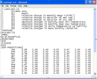
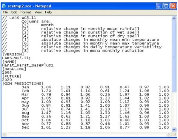
is useful for producing daily precipitation, radiation, and maximum and minimum daily temperatures at a station under present and future climate conditions (Racsko et al., 1991; Semnov and Barrow, 2002). The first version of LARS-WG was created as a tool for a statistical downscaling method in Budapest in 1990 (Racsko
et al., 1991). This model is composed of three
main parts; calibration of the model, assessment of model, and production of meteorological data. In order to run the LARS-WG model and downscale GCM data in future periods, two files have to be created; one file defines the behaviour of the climate in the past (*.WG) and the other is a climate change scenario file (*.Sta).
For generating a climate change scenario file for the LARS-WG model (Figures 2 and 3), climate change scenarios for three climate variables have to be calculated from AOGCM; changes in long-term average monthly precipitation of future period relative to baseline period (equation 1), changes in long-term average monthly duration of wet and dry spells of future period relative to baseline period, absolute change of long-term monthly average minimum and maximum temperature of future period relative to baseline period (equation 2), change of
fluctuations of daily temperature of future period relative to baseline period, and absolute changes of long-term monthly radiation of future period relative to baseline period are introduced under (*.sce) files to the LARS-WG model. It should be mentioned that daily data of AOGCM are needed for dry and wet period calculation and fluctuations of daily temperature, and for the remaining variables monthly data are satisfactory. For example, in Figure 2 if the changes of variables of dry and wet periods and fluctuations in daily temperatures for the future periods are supposed to be constant and other variables change, then the standard deviation of the daily time series of projected variables are close to observation data with differences in mean and corresponding data of future and observation data. If all scenarios of climate variables change, not only are corresponding daily variables of future parameters different to observation ones, but statistical parameters (mean and standard deviation) are different from the observation ones (Figure 3). In this study, the effect of the (abovementioned) two different modes downscaling by LARS-WG model on the runoff was studied. Figures 2 and 3 show different modes of climate change scenarios from LARS-WG model, respectively.
Fig. 3. Properties of climate change scenario II data file from LARS-WG model for the future period
2.3.3. Rainfall-runoff simulation
The IHACRES rainfall-runoff model was used to simulate the runoff of the basin under climate change. The IHACRES rainfall-runoff model was presented by Jakeman and Hornberger (1993). It is based on a non-linear loss module and linear
unit hydrograph module. The process of simulation includes converting precipitation and temperature (rk and tk) in each time step (k) to
effective rainfall (uk) by the non-linear module,
then converting to surface runoff by unit hydrograph linear modulus at the same time step (Figure 4).
Fig. 4. Generic structure of the IHACRES model, showing the conversion of climate time series data to effective rainfall using the non-linear module, and the non-linear module converting effective rainfall to stream flow time series
2.3.4. Performance functions
It is necessary to examine the performance of various models in simulating different variables. For this purpose, performance coefficient, coefficient of determination (R2), root mean
square error (RMSE), and standard error of bias were used in this study:
(5)
(6)
(7) In these equations, X is observation and simulated data, n is the number of data, index s indicates the simulated data, index o indicates the observation data. R2 represents a linear
relationship between simulated and observed data that varies between zero and one. The closer the
relationship indicated between the two variables. Since this criterion simulates only the behavioural pattern of the observation data, the other criteria such as RMSE and bias were used. Being less the results of these two performance coefficients means the minimum difference between observation and simulated data that shows higher performance in simulating process.
3. Results and Discussion
For simulating daily rainfall runoff in the basin using the IHACRES model the within observation period 1982-2008, the best calibration and validation periods were chosen to minimize the simulation error. The selection was based on the highest coefficient of determination R2 and the
lowest error (RMSE and bias) between observed and simulated runoff. To analyse, the input data
(temperature, precipitation and runoff observation) were selected from 12/1/1986 to 12/31/1994 for the calibration period and from 3/1/1993 to 12/31/2003 for the verification period. According to the results obtained from the implementation IHACRES model in Azam-Herat River and its climate conditions, the model performance to changes prediction in runoff state at about 70% were estimated. Figures 5 and 6 show the results of the IHACRES model in simulating runoff for calibration and validation periods in the study area.
However, considering the prevailing climatic conditions and characteristics of the studied area located in the dry area, the distribution of extreme rainfall and flow data, most models of rainfall -runoff under such situation do not enjoy the required performance.
Fig. 5. Time series of observed and simulated runoff in calibration period by IHACRES model (R2=0.783, RMSE =1.1)
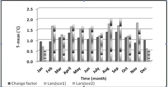
3.1. Temperature changes
Figure 7 shows the results of downscaled temperature by CF and two modes of LARS-WG methods in the form of the long-term monthly average difference between observed and future periods. According to Figure 7, both scenarios of LARS-WG show increasing temperature in all months except January and December to be higher than CF. In scenario I of the LARS-WG model, the greatest difference is in November (1oC) and
the lowest is in July (0.1oC). Scenario II of the
LARS-WG shows the highest difference of temperature in February, at around 0.8°C, and the
lowest in March. The CF method shows more of an increase in temperature in January and December in the future period relative to the observation period compared to the LARS-WG method. Generally, the highest temperature increase for the future period relative to the observation period is in August under scenario II of LARS-WG.
Fig. 7. Changes of long-term average monthly temperature of future period relative to observation period by three downscaling methods (change factor and two scenarios of LARS-WG)
3.2. Precipitation changes
Future changes in precipitation for the future periods relative to the observation period by two scenarios of LARS-WG and CF do not follow a uniform process, So that in some months the amount of precipitation of the future is greater than for the observation period, and in some months it is less than the observation period. As shown in Figure 8, the highest decrease of future precipitation by the CF relative to observation period will occur in March. The LARS-WG scenario I (with respect to the point that change in the variance remains constant in future), indicates precipitation increases in all months except May and November, where the amount of rainfall of the future period is less than the observation period. Scenario II, by applying changes of variance in future, shows a monthly increase in
Fig. 8. Long-term monthly average changes of precipitation of future period relative to observation period under three downscaling methods (change factor, LARS-WG I and II)
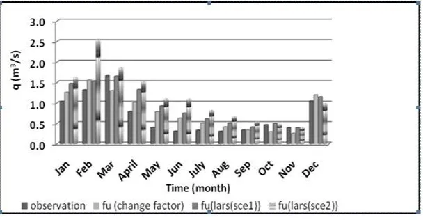
3.3. Runoff projection
Time series runoff of the Azam-Herat River Basin was projected by introducing precipitation and temperature time series downscaled by the CF method and two scenarios of LARS-WG to the calibrated with the IHACRES model for the period 2010-2039. Figure 9 shows long-term average monthly changes of runoff for the future period relative to the observation period under the CF method and two scenarios of LARS-WG. Scenario I of the LARS-WG model shows
increasing runoff in every month in which the maxima are in April and May. Similar to scenario I, scenario II projects an increase in runoff in all months except for November and December, and the maximum is February, which is very remarkable. The CF method projects an increase in runoff in all months except for October, November and March. Despite the low projection of precipitation in spring, these scenarios show an increase in runoff because of rising temperatures and melting snow and changes in soil permeability.
Fig. 9. Trend of long-term average monthly runoff for the period 2010-2039 by change factor and statistical downscaling method under climate change scenarios (change factor, statistical methods: LARS-WG: I and II, future period: fu)
4. Conclusion
In this study, the impact of climate change on runoff of the Azam-Herat River Basin located in Yazd province for the period of 2010-2039 under the uncertainty of downscaling methods was
downscaling methods for the climatic variables. The average temperature downscaled by three methods for the future period shows a difference of 3-4%; for precipitation this is about 30% and for runoff it is more than 30%. The results of this work revealed, however, that the calculation of CF is easy and simple for downscaling, but since in this method the fluctuations of the future period are the same as in the observation period, the projected runoff is not representative of actual future runoff. In the LARS-WG model, however, these fluctuations are well modelled. It should be noted that the LARS-WG requires more time, expertise and experience than the CF. Therefore, selecting the appropriate method for downscaling climate variables from the AOGCM model is highly dependent on the type of project. On the other hand, regarding the results of scenario II of LARS-WG, it is obvious that considering coupled variations and the mean of climatic variables’
impact on runoff would lead to better results. Finally, these results, compared with the results of Kamal et al., (2010), order to effect of different sources uncertainty. In both studies the improved results of simulated runoff are shown by statistical downscaling rather than the CF method. They also found the most effective source of uncertainty in runoff simulation of the study area to be related to the downscaling methods of AOGCM models. Therefore, this study investigated the uncertainty of downscaling methods (Lars-WG and CF).
References
Abbasi F., M. Asmari, H. Arabshahi, 2011. Climate Change Assissment over Zagros during 2010-2039 by using statistical Downscaling of ECHO-G Model. Environmental Research Journal. 5; 149-155.
Andrew Day, C., 2013. Statistically Downscaled Climate Change Projections for the Animas River Basin, Colorado, USA. Mountain Research and Development (MRD). 33; 75-84.
Arnell, N.W., N.S. Reynard, 1996. The effects of climate change due to global warming on river flows in Great Britain. Journal of Hydrology, 183; 397–424.
Babaeian, I., W.T. Kwon, E.S. Im, 2004. Application of weather generator technique for climate change assessment over Korea. Korea Meteorological Research Institute, Climate Research lab., 98p.
Barnett, T., R. Malone, W. Pennell, D. Stammer, B. Semtner, W. Washington, 2004. The effects of climate change on water resources in the West: Introduction and overview. Climatic Change, 62; 1–11.
Busuioc, A., R. Tomozeiub, C. Cacciamani, 2008. Statistical downscaling model based on canonical correlation analysis for winter extreme precipitation
events in the Emilia-Romagna region. International Journal of Climatology, 28; 449-464.
Chen, J., F.P. Brissette, R.L. Econte, 2011. Uncertainty of downscaling method in quantifying the impact of climate change on hydrology. Journal of Hydrology. 401; 190-202.
Croke, B.F.W., A.J. Jakeman, 2009. Use of the IHACRES rainfall-runoff model in arid and semi arid regions. Integrated Catchment Assessment and Management Centre. School for Resources, Environment and Society, and Centre for Resource and Environmental Studies, The Australian National University, Canberra, Australia.
Diaz-Nieto, J., R.L. Wilby, 2005. A comparison of statistical downscaling and climate change factor methods: impacts on low flows in the River Thames, United Kingdom. Climate change, 2; 245-268.
Dibike, Y.B., P. Coulibaly, 2005. Hydrologic impact of climate change in the Saguenay watershed: comparison of downscaling methods and hydrologic models. Journal of Hydrology, 307; 145–163.
Dunne Steel, Su. , P. Lynch, R. McGrath, T. Semmler, Sh. Wang, J. Hanafin, P. Nolan, 2008. The impacts of climate change on hydrology in Ireland. Journal of Hydrology, 356; 28–45.
Falloon, P., R. Betts, 2010. Climate impacts on European agriculture and water management in the context of adaptation and mitigation, the importance of an integrated approach. Science of the Total Environment, 408; 67-87.
Hughes, M.K., H.F. Diaz, 2008. Climate variability and change in the drylands of Western North America. Global and Planetary Change, 64; 111–118.
Huth, R., 2005. Downscaling of Humidity Variables: A Search for Suitable Predictors and Predictands. International Journal of Climatology, 25; 243–250. IPCC, 2007. Summary for Policy markers, in: Climate
Change 2007. Solomon, S., D. Qin, M. Manning, Z. Chen, M. Marquis, K.B. Averyt, M. Tignor, H.L. Miller (eds.) (2007) Climate Change 2007: The Physical Science Basis, Contribution of Working Group I to the Fourth Assessment Report of the Intergovernmental Panel on Climate Change, Cambridge University Press, Cambridge, 1-18. IPCC-TGCIA, 2007. General guidelines on the use of
scenario data for climateimate impact and adaptation assessment, K. Alfsen, E. Barrow, B. Bass, X. Dai, P. Desanker, S.R. Gaffin, F. Giorgi, M. Hulme, M. Lal, L.J. Mata, L.O. Mearns, J.F.B. Mitchell, T. Morita, R. Moss, D. Murdiyarso, J.D. Pabon-Caicedo, J. Palutikof, M.L. Parry, C. Rosenzweig, B. Seguin, R.J. Scholes, P.H. Whetton, Task Group on Data and Scenario Support for Impact and Climate Assessment.
Jakeman, A.J., G.M. Hornberger, 1993. How Much Complexity Is Warranted in a Rainfall-Runoff Model? Water Resources Research, 29; 2637-2649.
Kilsby, C.G., P.D. Jones, A. Burton, A.C. Ford, H.J. Fowler, C. Harpham, P. James, A. Smith, R.L. Wilby, 2007. A daily weather generator for use in climate change studies. Environmental Modelling and Software, 22; 1705-1719.
approach to equilibrium. Climate Dynamics, 20; 635-661.
Kim, S.J., G.M. Flato, G.J. Boer, N.A. McFarlane, 2002. A coupled climate model simulation of the Last Glacial Maximum, Part 1: transient multi-decadal response. Climate Dynamics, 19; 515-537.
Leander, R., T.A. Buishand, 2007. Resampling of regional climate model output for the simulation of extreme river flows. Journal of Hydrology, 332; 487-496. doi:10.1016/j.jhydrol.2006.08.006.
Liu, Q., B. Cui, 2011. Impacts of climate change/variability on the streamflow in the Yellow River Basin, China. Ecological Modelling, 222; 268-274.
Massah Bavani, A.R., S. Morid, 2006. Impact of climate change on the water resources of zayanderud basin–
Iran. Journal of science and Technology of Agriculture and Natural Resources, Water and Soil Science. 9; 17-28.
Mearns, L.O., C. Rosenzweig, R. Goldberg, 1996. The effect of changes in daily and interannual climatic variability on CERES-Wheat: a sensitivity study. Climatic Change, 32; 257–292.
Minville, M., F. Brissete, R. Lecont, 2008. Uncertainty of the impact of climate change on the hydrology of the Nordic watershed. Journal of Hydrology, 358; 70-83. Mitchell, T.D., 2003. Pattern Scaling: An Examination of
Accuracy of the Technique for Describing Future Climates. Climatic Change, 60; 217-242.
Nnyaladzi, B., Y. Brent, 2010. Rainfall variability and trends in semi-arid Botswana. Implications for climate change adaptation policy. Applied Geography, 30; 483-489. doi:10.1016/j.apgeog. 2009.10.007.
Ramos, M.C., J.A. Martinez-Casasnovas, 2006. Trends in precipitation concentration and extremes in the
Mediterranean Penedes-Anoia region, NESpain. Climatic Change, 74; 457–474. doi: 10.1007/s10584-006-3458-9.
Reynard, N.S., C. Prudhomme, S. Mcrooks, 2001. The flood characteristics of large U.K. rivers: potential effects of chaning climate and landuse. Climate change, 48; 343-359. doi: 10.1023/A:1010735726818
Robera, N., J.V. Hardenberg, A. Provenzale, 2005. Rainfall downscaling and flood forecasting: a case study in the Mediterranean area. Journal of Natural Hazards and Earth System Sciences, 6; 611-619.
Semenov, M.A., 2007. Developing of high-resolution UKCUP02-based climate change scenarios in the UK. Journal of Agricultural and Forest Meteorology, 144; 127-138.
Sperna Wiland, F.C., L.P.H. Van Beek, A.H. Weerts, M.F.P. Bierkens, 2011. Extracting information from an ensemble of GCMs to reliably assess future global run off change. Journal of Hydrology. 412; 66-75.
Tabor, K., J. Willams, 2010. Global downscaled climate projections for assessing the conservation impacts of climate change. Ecological Applications, 20; 554-565. Tompkins, E.L., 2005. Planning for climate change in
small islands: insights from national hurricane preparedness in the Cayman Islands. Global Environmental Change, 15; 139–149.
Wilby R.L., I. Harris, 2006. A frame work for assessing uncertainties in climate change impacts: low flow scenarios for the River Thames, UK. Water Resources Research, 42; 1-10.