The Monetary Policy, Credit Constraint and Spatial
Distribution of Economic Activity:
A Contribution of New Economic Geography
*Ahmad Jafari Samimi1, Saeed Rasekhi2, Seyed Peyman Asadi*3
Received: 2017, November 5 Accepted: 2018, January 2
Abstract
his paper investigates the effect of monetary policy on the distribution of economic activity and agglomeration economies within a country. The considered channel for this effectiveness is the availability of credit to firms in various regions and the effects on the labor and consumer welfare. For this purpose, data for manufacturing firms located in 30 different provinces in Iran during 2007 and 2014 gathered. The empirical results from spatial panel data show that beside conventional channel of effectiveness through consumer and labor force utility function, regional monetary policy implication through uneven distribution of regional loanable banking fund seems to be substantial centripetal force. In terms of most well-known NEG variable, uneven regional accessibility of credit market has opposite regional implication as trade freeness. While the former leads to more concentration of economic activity across space, the latter tends to drive dispersion. It is assumable that monetary policy reduce the impact of credit constraints on firms but the degree of credit availability in regions is a significant driver for concentration of economic activity. The result shows the importance of accessibility to banking loans on distribution of economic activities within the country.
Keywords: Monetary Policy, Credit Constraint, Agglomeration, Dispersion,Spatial Panel Data,Dynamic Panel Data, Iran.
JEL Classification: E52, E51, E44, R11.
1. Introduction
Empirical studies shows that there is an inherent differences in the regional wages in a growing number of countries (Duranton and
* The article is extracted from PhD dissertation of Corresponding author, University of Mazandaran, Babolsar, Iran.
1. Faculty of Economics & Administrative Sciences, University of Mazandaran, Babolsar, Iran ([email protected]).
2. Faculty of Economics & Administrative Sciences, University of Mazandaran, Babolsar, Iran ([email protected]).
3. Faculty of Economics & Administrative Sciences, University of Mazandaran, Babolsar, Iran (Corresponding Author: [email protected]).
Monastiriotis, 2002; Azzoni and Servo, 2002; Maier and Weiss, 1986). Identical workers in terms of various measure of human capital such as education and experience are paid differently for identical work depending upon the region in which they work (Beenstock and Felsenstein, 2008). However, some studies suggest that just as there is convergence failure at the international level (Barro et al., 1991), there is also convergence failure within countries (Beenstock and Felsenstein, 2010). It seems surprising as trade is likely to be freer within countries than between them and capital and labor force which assume has the same characteristic are likely to be more mobile within countries.
To explain the discovery of convergence failure at the international level new theories, such as endogenous growth theory (e.g. Grossman and Helpman, 1993) was generated. To explain the fact of regional convergence failure the same has happened and new theory such as new economic geography (NEG) try to answer this surprise (Beenstock and Felsenstein, 2010).
Initially originated from international trade theory, New Economic Geography (NEG), is an attempt to find factors which shape firms and workers’ location behavior and to explain the formation of a large variety of economic agglomeration (or concentration) in geographical space (Fujita and Krugman, 2004).
Even though the traditional location choice factors have been changing in time, initial advantages, low transportation costs, accessibility to market and skilled labor, are still significant forces generating agglomeration economies (Fuijita and Thisse, 1996; McCann, 2001; Parr, 2002; Capello, 2007).
According to the location patterns of manufacturing industry, on one hand firms are likely to concentrate within the metropolitan areas when they have access to a larger markets and lower transport costs and on the other hand, urban areas provide a wide array of final goods and specialized labor market pool which make them attractive to consumers and workers. As a result of the process, Agglomeration economies are the result of cumulative processes involving both the supply and demand sides (Krugman, 1980; 1991; Ottaviano and Thisse, 2003; Puga, 2010).
In this paper we examine the effect of monetary policy on the distribution of economic activity within the country. For this purpose, data for manufacturing firms located in 30 different provinces of Iran during 2007-2014 are gathered. The innovative approach of this study is regarding to inclusion of monetary policy into NEG models, which basically are silent toward this kind of macroeconomic policy. The way of effectiveness of monetary policy is loanable banking resource in each regions and though the availability of credit to firms in various region. High degree of spatial concentration in the financial market in developed and metropolitan areas (Palmberg, 2012) faced firms in less developed areas with critical performance challenges as informational disadvantages (Danielson and Scott; 2004, Petersen and Rajan; 1994, 1997), limited source and higher cost of borrowing (Arena and Dewally, 2012; Smith, 1987; Petersen and Rajan, 1994), higher risk of asset substitutions (Leland and Pyle, 1977), and inflexibility of capital structure, sub-optimally lower leverage ratio (Arena and Dewally, 2012; Mayers, 1977), lead them to have a poorer performance and will change to a significant obstacle to their expansion, join new markets and export orientation production (Fauceglia, 2015). Due to such critical obstacles unevenness distribution of regional loanable banking fund seems to be substantial centripetal force.
It is assumable that monetary policy expansion reduce the impact of credit constraints on firms (Orlowski, 2015) but the degree of credit availability in regions is a significant driver for concentration of economic activity. Besides monetary policy has a direct effect on the labor force and consumer utility which affect the migration decision.
the economic agglomeration and provides a framework to analyze the effect of monetary policy on the spatial dispersion and concentration. In the section 3 explanation of econometric model, variables, data and empirical result are presented. Finally, last section devoted to conclusion and policy implications.
2. Literature
borrow more from local banks and repeatedly borrow from the same banks instead of frequently changing lenders (Arena and Dewally, 2012). In additions instead of short-term debt, to raise debt capital banks might be more likely to offer small area firms longer-term debt which might increase the underinvestment problem and sub-optimally lower leverage than urban firms (Arena and Dewally, 2012; Mayers, 1977). During monetary contraction availability of credit has more detrimental effect on firm’s performance (Atanasova and Wilson, 2004; Choi and Kim, 2005 and Mateut et al., 2006). Besides firms with high levels of short-term debt, which are vulnerable to financial crises, reduce the provision of trade credit during periods of contraction in bank credit which may be highly risky (Love et al., 2007). There is some evidence shows that small firms did not receive any alternative source of sufficient credit to compensate for the decline in bank loans during a monetary squeeze (Marotta, 1997). By focusing on leverage and debt maturity there is expressive interplay between geographical location of firms and the structure of corporate debt. Empirical finding of the effect of proximity on firms equity shows that firms in less developed area cannot easily change their capital structure from debt to equity (or vice versa) to reduce their cost of capital (Loughran, 2008).
credit to their customer (Tsuruta, 2014; Montoriol-Garriga, 2013) and not able to join new markets and export orientation production (Fauceglia, 2015).
Krugman and Venables (1990) provide one of the first relevant formal contributions about the functioning of NEG models in predicting agglomeration in a framework of economic integration (Ascani et al., 2012). The core-periphery model has two main variants. The footloose-labor variant (Krugman, 1991) and the vertical-linked-industries variant (Venables, 1996). In the first one agglomeration forces driven by inter-regional labor migration within a single sector and the motivation of the migration is the differences in the regional real wage. In the latter one agglomeration driven by intersectoral migration within each region; and the intersectoral nominal wage differences motivate migration (Baldwin, 2001).
Fujita et al. (1999) –FKV–provides a comprehensive review on the standard CP model. In the initial stage of CP model there is two symmetric region, two factors of production and two sector of manufactures and agriculture. Manufacture sector is a Dixit-Stiglitz monopolistic competition with increasing returns whereas the agriculture sector has a perfectly competitive production function with constant return which produce homogenous good. Production in both sector is tradable but in the monopolistic competition there is a fractional trade cost which assumed as iceberg trade cost and in the perfectly competitive sector is costless.
Dixit-Stiglitz monopolistic competition emerges as a market structure determined both by consumers’ preferences for variety and firms’ fixed requirements for limited productive resources. Description of such quality is on the demand side, preference of consumers for variety and on the supply side, internal economies of scale for each good, but no economies of scope across goods (Fujita and Thisse, 2009).
Representative consumer preferences is a Cobb-Douglas function of the consumption of agriculture and manufacture production:
𝑈 ≡ 𝐶𝑥𝜇𝐶𝑧1−𝜇; 𝐶𝑥 ≡ (∫ 𝑐𝑖1−
1 𝜎 𝑛+𝑛∗
𝑖=0 )
1 1−1𝜎
Where 𝐶𝑥 represents a composite index of the consumption of manufacture good and 𝐶𝑧 is the consumption of agriculture good. 𝜇 is
a constant representing the expenditure share of manufactured good, n and n* are the number (mass) of varieties in two regions, and 𝜎 represents the elasticity of substitution between any two varieties of manufactured goods.
Regional supplies of agriculturist (A) as well as the global supply of workers (L) are fixed, but the inter-regional distribution of L is endogenous and determined by regional real wage differences.
Assuming 𝑠𝐿 the share of labour in the north, 𝐿 and 𝐿𝑤 are the north work supply and total work supply,𝜔, 𝜔∗, 𝜔̅ are the northern, southern and average real wages. P is the north region price index with 𝑝𝑧 being the price of manufactured product and 𝑝𝑖 being the price of variety i; the exposition of migration equation in the KFV model has showed as below;
𝑠̇𝐿= (𝜔 − 𝜔̅)𝑠𝐿; 𝑠𝐿≡𝐿𝐿𝑤 ; 𝜔 = 𝑊
𝑃 ; 𝜔̅ ≡ 𝑠𝐿𝜔 + (1 − 𝑠𝐿)𝜔∗ (2)
𝑃 ≡ 𝑝𝑧1−𝜇(∫𝑛+𝑛∗𝑝𝑖1−𝜎𝑑𝑖
𝑖=0 )
𝜇/(1−𝜎)
(3)
By optimization of Eq.1 a constant division of expenditure between manufactured goods (X) and agriculture good (Z), CES demand functions for manufactured good varieties, agricultural good and expenditure function (E) can be written as:
𝑐𝑗 =
𝑝𝑗−𝜎𝜇𝐸
∫𝑖=0𝑛+𝑛∗𝑝𝑖1−𝜎𝑑𝑖; (4)
𝐶𝑧 = (1−𝜇)𝐸𝑝
𝑥 (5)
𝐸 = 𝑤𝐿 + 𝑤𝐴𝐴 (6)
symmetry, a small displacement between two regions may change the size of the market in both region. By changing the size of the market, firms sales in north raise and fall in the south. This encourages northern firms to hire workers, southern firms to fire workers, and thus the small migration shock encourages more migration (Baldwin, 2001).
On the supply side, since A is immobile and both region produce some agricultural good, free trade in agricultural good equalizes wage rates, w and w* in two regions. Regarding price of manufactured and agricultural products by choosing units of agricultural product such that one unit of agriculturist (A) is required per unit of agricultural product, 𝑝𝑧 = w = w ∗= 1. Also measuring manufactured products in
units such that 𝑎𝑥 = (1 −𝜎1) the price of a northern manufactured
product variety in its local and export markets are 𝑝 = 𝑤 and 𝑝∗= 𝑤𝜏 respectively. Also we have;
𝜋 =𝑤(𝐿−𝑛𝐹)(𝜎−1)𝑛 (7)
The free entry condition requires n to rise to the point where 𝜋 = 𝑤𝐹. Using Eq. 7 we have;
𝑛 =𝜎𝐹𝐿 ; 𝑥̅ = 𝜎𝐹 (8)
Where 𝑥̅ is the equilibrium firm size of a typical firm in manufacturing sector. Eq. (8) serve as the second agglomeration force in the model which views migrants as workers. An exogenous increase in L and corresponding decrease in L* would raise n and lower n*. Since locally produced varieties attract no trade cost the shift in n’s would, other things equal (in particular the w’s), raise the north’s relative real wage, This in turn would tend to pull in more migrants. This is called cost-linked circular causality, or forward linkages (Baldwin, 2001).
whether to supply the home region and export to the other regions. Matsuyama (2005) introduced the effect of credit constraints in a general way. In this framework as a consequence of imperfections in financial contracting firms can only borrow a fraction (𝜃) of their operating profit which it correspond to maximum amount to cover fixed production expenditure and exporting cost, 𝑓 and 𝑓𝑥, though internal funds play crucial role to finance remaining part.
An exporting firm must consider an additional fixed exporting cost 𝑓𝑥 and an iceberg trade cost 𝜏 , where 𝜏 > 1 of each good must be shipped in order for one good to reach the export destination. It is assumable regarding Melitz (2003) type models that 𝜏𝜎−1𝑓𝑥 > 𝑓 and the cut-off productivity level for exporting profitably 𝜑𝑥 is higher than the productivity threshold to earn nonnegative profits in the domestic market 𝜑∗ .
For exploiting greater market firms should overcome potential financing obstacles. Only firms that meet the following export profitability condition (9) and the credit constraint condition (10) will therefore become exporters and can gain from grater market:
𝜏1−𝜎 𝜇
𝜎𝐸(𝑃𝜌)𝜎−1(𝜑)𝜎−1 ≥ 𝑓𝑥 (9)
𝜃 [1𝜎(1 + 𝜏1−𝜎)𝑟
𝑑(𝜑)] ≥ 𝑓 + 𝑓𝑥− 𝜔 (10)
Accruing positive export gain due to the export profitability condition (9) need minimum level of exporter productivity of 𝜑𝑥=
𝜏 𝑃𝜌(
𝜎𝑓𝑥 𝜇𝐸)
1
𝜎−1. In additions, neutralizing credit constraint condition (10),
granting external finance and availability of internal funds yields the minimum cutoff firm productivity of;
𝜑𝑥(𝜔, 𝜃) = 𝑃𝜌1 ( 𝜎(𝑓+𝑓𝑥−𝜔) 𝜃𝜇𝐸(1+𝜏1−𝜎))
1
𝜎−1 (11)
Only firms that draw a firm productivity at least as high as 𝜑 ≥ 𝑚𝑎𝑥[𝜑𝑥, 𝜑𝑥(𝜔, 𝜃)] are able to export profitably and secure access to
Eq (4) to (6) and (8) gives the market clearing condition as below;
𝑤𝑥̅ = 𝑅; 𝑅 ≡𝑛𝑤1−𝜎𝑤1−𝜎+∅𝑛𝜇𝐸∗𝑤∗1−𝜎+∅𝑛𝑤∅𝑤1−𝜎1−𝜎+𝑛𝜇𝐸∗𝑤∗∗1−𝜎 (12)
Where R is a mnemonic for ‘retail sales’ and ∅ = 𝜏1−𝜎 measures
‘free-ness’ of trade. Variation of the free-ness of trade rises from ∅ = 0 which means infinite trade costs to ∅ = 1 which mean zero trade costs. Eq (12) serve as stabilizing and dispersion force in the model. By moving a small mass of L from south to north and raise n and lower n*, from the expression for R, this tends to increase competition for consumers among northern firms, thus lowering R. Though northern firms would have to pay a lower nominal wage. Consequently the drop in w and corresponding rise in w* would make north less attractive to workers. In the core-periphery literature, this dispersion force is commonly called the ‘local competition’ effect or ‘market-crowding’ effect (Baldwin, 2001).
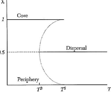
The relation between the level of trade costs and agglomeration and dispersion forces can be conveniently summarized by Fig. 1. Indeed, as pointed out by Baldwin et al., 2003, the scenario depicted by Fig. 1 is broadly consistent with most NEG models, both static (e.g. Krugman 1991a; Krugman and Venables, 1995; Venables, 1996; Puga, 1999; Ottaviano et al., 2002) and dynamic ones (e.g. Baldwin, 1999; Martin and Ottaviano, 1999, 2001; Baldwin et al., 2001).
Figure 1 portrays the possible long-run spatial configurations of a simple economy consisting of two regions with no inner spatial dimensions. The figure illustrate how the number and type of equilibria vary with the level of trade cost 𝑇. The vertical axis measures 𝜆, the share of firms located in one regions, solid and dotted lines denote stable and unstable equilibria respectively. At every level of trade costs there exists a symmetric diversified equilibrium (Neary, 2001). In the figure the extent of trade freeness, T is represented on the horizontal axis while the share of firms located in one of the regions appears on the vertical one. Trade freeness is an inverse measure of trade costs: 𝑇 = 1 means autarky; 𝑇 = 0 means free trade. Heavy solid lines indicate long-run outcomes. These are geographical distributions of firms towards which the economic system evolves as pointed out by the vertical arrows. Fig. 1 then shows that for low trade freeness (𝑇 > 𝑇𝑠) a dispersed geographical distribution of firms is the only long-run outcome. For high trade freeness (𝑇 < 𝑇𝐵) agglomeration in either region is the only long-run outcome. For intermediate values of trade freeness (𝑇𝐵 < 𝑇 < 𝑇𝑆) both dispersion and agglomeration can emerge in the long run, so history and policy have a potential role in influencing which equilibrium prevails (Ottaviano, 2003; Neary, 2001).
What should be emphasized is that new economic geography theory does leave space for other factors such as economic policies and geography to play their roles. As stated by Neary (2001), when trade costs are in certain range, both agglomeration and diversification are possible equilibriums, so history and policy have a potential role in influencing which equilibrium prevails.
3. Econometric Model and Data Explanation The model adopts the following form:
𝐴𝐺𝑖𝑡 = 𝛽0𝐴𝐺𝑖,𝑡−1+ 𝛽1𝐶𝑅𝑖𝑡+ 𝛽2𝑊𝑖𝑡+ 𝛽3𝐶𝑃𝐼𝑖𝑡+ 𝛽4𝑇𝑅𝑉𝑖𝑡+ 𝛽5𝐺𝐷𝑃𝐶𝑖𝑡+ 𝛽6𝐻𝐶𝑖𝑡+ 𝛽7𝐺𝐵𝑖𝑡+ 𝛽8𝑈𝐷𝑖𝑡+
𝜀𝑖𝑡 (13)
wage rate, (𝐶𝑃𝐼) regional consumer price index, (𝑇𝑅𝑉) regional share of transport and communication vale added as an index of freeness of trade, (𝐺𝐷𝑃𝐶) regional GDP per capita to capture the market size effect, (𝐻𝐶) regional human capital quality, (𝐺𝐵) regional government budget and (𝑈𝐷) is an index for urban development.
Economic policies have their spatial impacts. Particularly, we will test the impact of two types of policies on industrial agglomeration, monetary policy and the government involvement in regional economic activities. Monetary policy is represented by credit available in each regions. Obviously, different credit availability in various regions is expected to encourage regional industrial agglomeration. To investigate the local government involvement in regional economic activities, regional government expenditure included in the model which we expect to weaken the regional industrial agglomeration. Lag independent variables are used as proxy variables which shows the importance of history and previous industrial structure and shows the effect of history and geography on regional industrial agglomeration (Chen et al., 2008).
firms, this variables should be positively related to regional share in industrial activity.
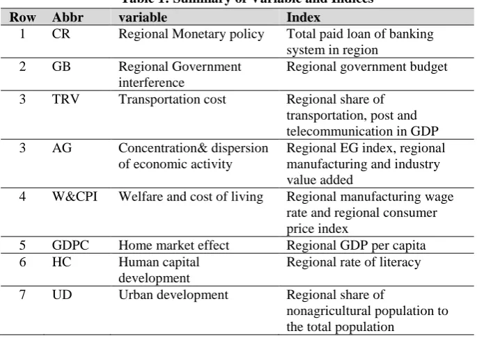
Table 1: Summary of Variable and Indices
Row Abbr variable Index
1 CR Regional Monetary policy Total paid loan of banking system in region
2 GB Regional Government
interference
Regional government budget
3 TRV Transportation cost Regional share of
transportation, post and telecommunication in GDP 3 AG Concentration& dispersion
of economic activity
Regional EG index, regional manufacturing and industry value added
4 W&CPI Welfare and cost of living Regional manufacturing wage rate and regional consumer price index
5 GDPC Home market effect Regional GDP per capita
6 HC Human capital
development
Regional rate of literacy
7 UD Urban development Regional share of
nonagricultural population to the total population
4. Estimation and results:
In estimating equation (13), the disturbance vector is assumed to have random region effects as well as spatially auto-correlated residual disturbances;
𝜀𝑡= 𝜇 + 𝜻𝑡 (14)
𝜻𝑡 = 𝜌𝑊𝜻𝑡+ 𝜂𝑡 (15)
where 𝜀𝑡= (𝜀1𝑡, … , 𝜀𝑁𝑡)′, 𝛇𝑡 = (𝛇1𝑡, … , 𝛇𝑁𝑡)′ and 𝜇 = (𝜇𝑡, … , 𝜇𝑁)′ denotes the vector of random region effects, which are assumed to be i.i.d. (0,𝜎𝜂2). 𝜌 is the scalar spatial autoregressive coefficient
𝜉𝑡= (𝐼𝑁− 𝜌𝑊)−1𝜉𝑡 = 𝐴−1𝜂𝑡 (16)
Where 𝐴 = 𝐼𝑁− 𝜌𝑊 and 𝐼𝑁 is an identity matrix of dimension N.
Also by rewriting (14) into vector form we have:
𝜀 = (𝜄𝑇⨂𝐼𝑁)𝜇 + (𝐼𝑇⨂𝐴−1) 𝜂 (17)
Where ι𝑇 is a vector of ones of dimension T and 𝐼𝑇 is an identity matrix of dimension T.
The variance-covariance matrix of 𝜀 is as follow:
𝛺𝜀 = 𝐸[𝜀𝜀′] = 𝜎
𝜇2(𝐽𝑇⨂𝐼𝑁) + 𝜎𝜂2[𝐼𝑇⨂(𝐴′𝐴)−1] (18)
Where 𝐽𝑇 is a matrix of one of dimension T. Following Baltagi, Song,
and Koh (2003), this variance–covariance matrix can be rewritten in such a way that
𝛺𝜀 = 𝜎𝜂2{𝐽
𝑇⨂[𝑇∅𝐼𝑁+ (𝐴′𝐴)−1] + 𝐸𝑇⨂(𝐴′𝐴)−1} = 𝜎𝜂2∑𝜀 (19)
Under the assumption of normality, the log-likelihood for our model, conditional on 𝛿, becomes (Baltagi, Song, and Koh 2003):
ℒ(𝛾, 𝜎𝜂2, ∅, 𝜌|𝛿) = −𝑁𝑇2 ln(2𝜋𝜎𝜂2) −12𝑙𝑛| ∑𝜀 | −2𝜎1 𝜂2𝑒
′∑
𝜀−1𝑒 = 𝑁𝑇
2 ln(2𝜋𝜎𝜂2) − 1
2𝑙𝑛| 𝑇∅𝐼𝑁+ (𝐴′𝐴)−1 | + 𝑇−1
2 𝑙𝑛| 𝐴′𝐴 | −
1 2𝜎𝜂2𝑒
′∑
𝜀−1𝑒 (20)
Table 2: Spatial Panel Data and Dynamic Panel Estimation:
Methods Spatial Error Panel Data estimation GMM Panel Data estimation Variable model 1* model 2** model 3*** model 1* model 2** model 3***
EG(-1) 0.17132
(0.053) ---- ----
0.124848
(0.0241) ---- ----
industry(-1) ---- 0.1396
(0.028) ---- ----
0.616844 (0.0000) ----
manufacturing(-1) ---- ---- 0.05651
(0.154) ---- ----
0.173883 (0.0000)
Provincial credits 2.2E
(0.001) 0.06509 (0.0655) 0.00028 (0.0978) 9.56E (0.0821) 0.058326 (0.0000) 2.41E (0.0000)
Wage 0.0008
(0.010) 407566 (0.0000) 15004 (0.083) 5.75E (0.0007) 73.56827 (0.4961) 0.311513 (0.0000)
CPI -0.00599
(0.0000) -165692 (0.0177) -179108 (0.0000) -0.000825 (0.0000) -126376.5 (0.2106) 74.55068 (0.0012) Transport value added 2.87E-09 (0.0733) 0.9590 (0.0975) 0.9895 (0.0001) 1.73E-09 (0.0733) 0.232396 (0.0050) 0.000126 (0.0000)
Human Capital 2.27E
(0.045) 1849.104 (0.0022) 116.24 (0.0288) 2.42E (0.0299) 1683.699 (0.0000) 0.241977 (0.3241)
Urban development 0.151
(0.540) 9.26E (0.0000) 6.16E (0.346) 1.43 (0.0000) 8.83E (0.0242) 296253.2 (0.0008)
GDP Percapita 0.0059
(0.181) 160922 (0.0142) 17667 (0.0000) -3.93E (0.767) 115.81 (0.0022) 0.046886 (0.0001)
Government budget 1.42E
(0.598) 0.2993 (0.840) -0.05871 (0.930) -3.93E (0.767) 4.1238 (0.0001) 0.000307 (0.0118)
J-Statistic ---- ---- ---- 14.51065 (0.2692) 6.643467 (0.466921) 7.845729 (0.448683) 𝝆 0.2008 (0.001) -0.22071 (0.1814) 0.23781
(0.0541) ---- ---- ----
𝝈𝟐 0.001
(0.000) 4.08 (0.001)
5.55
(0.0001) ---- ---- ----
Note; () shows p-values. * Dependent variable EG index
** Dependent variable industry value added *** Dependent variable manufacturing value added
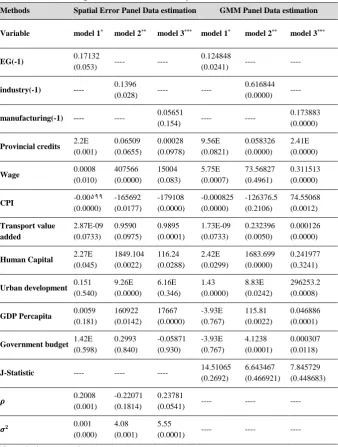
autoregressive disturbance in the model and confirms the impact of cross-region spillovers on the spatial distribution of industrial activity. Lag dependent variable has included in the model to assess the impact of history of the region. According to the result in both estimations and models previous situation has a direct relationship with the current situation.
Generally, the signs of all the coefficients of the explanatory variables seem to be consistent with the theoretical expectations. Thus, the impact of provincial credit which measured by loan paid in each region on agglomeration forces seems to be positive throughout, so that it might be inferred that availability of credit have a significant potential for concentration of industrial activities. Hence, it might be asserted that degree of concentration might be increasing due to uneven distribution of banking paid loan in various regions. This results also in the GMM estimation are same. The positive relationship between the provincial credits and agglomeration can be explained by several reasons which have presented in details in the literature review.
Regional manufacturing wage rate and consumer price index as the welfare index of labor force and consumer are the determinant factor in the migration equation. As the results of spatial estimations in table (2) shows that higher regional manufacturing wage rate consistent with higher degree of concentration, while higher regional consumer price strengthen the dispersion forces. GMM estimation also confirm the results of spatial estimation with this difference that regional manufacturing wage rate in model 2 is not statistically significant and regional consumer price index in model 3 has a positive sign.
Human capital, urban development, GDP Per capita has a positive effect on the concentration of industrial economic activity. While this variable can be seen to represent the development level of various province, it can be attractive to the workers and interpreted as the potential of the consumption for the industries. More importantly higher GDP per capita would have a chance of good access to the market or what called as home market effect (Combes and Overman, 2003). In the table (2) spatial estimation all this mentioned variables have the positive impact on the agglomeration but in the model 1 and 3 urban development and model 1 GDP per capita are not statistically significant. In the GMM estimation despite human capital in model 3 which is not statistically significant, all variables have the positive impact and consistent sign with the theoretical background.
5. Summary and Conclusion
and have better access to financial resources. In fact Policy makers must consider the fact that the uneven distribution of financial resources can have a serious impact on the economic performance of marginalized areas. Also it is important to say that financial issues are just one of many factors a firm has to take into account when selecting their location. This firms might favor their location because of specific industry geographical clustering, convenient access to intermediate inputs, proximity to suppliers or customers, state tax policy and considerations, or local favoritism by public officials, although access to financial resources can affect them substantially.
References
Alecke, B., Alsleben, C., Scharr, F., & Untiedt, G. (2008). Geographic Concentration of Sectors in the German Economy: Some Unpleasant Macroeconomic Evidence for Regional Cluster Policy. In U. Blien, & G. Maier, The Economics of Regional Clusters. Networks, Technology
and Policy, New Horizons in Regional Science (209-233).
Cheltenham: Edward Edgar Publishing.
Arena, M. P., & Dewally, M. (2012). Firm Location and Corporate Debt. Journal of Banking & Finance, 36(4), 1079-1092.
Artis, M., Curran, D., & Sensier, M. (2011). Investigating Agglomeration Economies in a Panel of European Cities and Regions. Retrieved from
http://eprints.lse.ac.uk/58459/1/__lse.ac.uk_storage_LIBRARY_Seco ndary_libfile_shared_repository_Content_SERC%20discussion%20pa pers_2011_sercdp0078.pdf.
Ascani, A., Crescenzi, R., & Iammarino, S. (2012). New Economic Geography and Economic. WP1/02 Search Working Paper, Retrieved from http://www.ub.edu/searchproject/wp-content/uploads/2012/02/WP-1.2.pdf.
Azzoni, C. R., & Servo, L. (2002). Education, Cost of Living and Regional Wage Inequality in Brazil. Papers in Regional Science, 81(2), 157-175.
Bacolod, M., Blum, B. S., & Strange, W. C. (2009). Skills in the City.
Journal of Urban Economics, 65(2), 136-153.
Baldwin, R. E. (1999). Agglomeration and Endogenous Capital.
European Economic Review, 43(2), 253-280.
Baldwin, R. E. (2001). Core-periphery Model with Forward-looking Expectations. Regional Science and Urban Economics, 31(1), 21-49.
Baldwin, R. E., Martin, P., & Ottaviano, G. I. (2001). Global Income Divergence, Trade, and Industrialization: The Geography of Growth Take-offs. Journal of Economic Growth, 6(1), 5-37.
Baldwin, R., Forslid, R., Martin, P., Ottaviano, G., & Robert-Nicoud, F. (2003). Public Policies and Economic Geography. Princeton: PUP.
Baltagi, B. H., Song, S. H., & Koh, W. (2003). Testing Panel Data
Regression Models with Spatial Error Correlation. Journal of Econometrics, 117(1), 123-150.
Barro, R. J., Sala-i-Martin, X., Blanchard, O. J., & Hall, R. E. (1991). Convergence across States and Regions. Retrieved from https://www.econstor.eu/bitstream/10419/160551/1/cdp629.pdf. Bebchuk, L. A., & Cohen, A. (2003). Firms’ Decisions Where to Incorporate. The Journal of Law and Economics, 46(2), 383-425.
Becker, B. (2007). Geographical Segmentation of US Capital Markets.
Journal of Financial Economics, 85(1), 151-178.
Beenstock, M., & Felsenstein, D. (2008). Regional Heterogeneity, Conditional Convergence and Regional Inequality. Regional Studies,
Beenstock, M., & Felsenstein, D. (2010). Marshallian Theory of Regional Agglomeration. Papers in Regional Science, 89(1), 155-172.
Berger, A. N., Miller, N. H., Petersen, M. A., Rajan, R. G., & Stein, J. C. (2005). Does Function Follow Organizational Form? Evidence from the Lending Practices of Large and Small Banks. Journal of
Financial Economics, 76(2), 237-269.
Berliant, M., Reed, R. R., & Wang, P. (2006). Knowledge Exchange, Matching, and Agglomeration. Journal of Urban Economics, 60(1), 69-95.
Boschma, R. (2005). Proximity and Innovation: a Critical Assessment.
Regional Studies, 39(1), 61-74.
Brealey, R., Leland, H. E., & Pyle, D. H. (1977). Informational Asymmetries, Financial Structure, and Financial Intermediation. The Journal of Finance, 32(2), 371-387.
Brickley, J. A., Linck, J. S., & Smith, C. W. (2003). Boundaries of the Firm: Evidence from the Banking Industry. Journal of Financial Economics, 70(3), 351-383.
Capello, R. (2007). Regional Economics. New York: Routledge.
Charlot, S., & Duranton, G. (2004). Communication Externalities in Cities. Journal of Urban Economics, 56(3), 581-613.
Chen, Z., Jin, Y., & Lu, M. (2008). Economic Opening and Industrial Agglomeration in China. In Economic Integration in East Asia:
Perspectives from Spatial and Neoclassical Economics (276-280).
Cheltenham: Edward Edgar Publishing Limited.
Coval, J. D., & Moskowitz, T. J. (1999). Home Bias at Home: Local Equity Preference in Domestic Portfolios. The Journal of Finance,
54(6), 2045-2073.
Danielson, M. G., & Scott, J. A. (2004). Bank Loan Availability and Trade Credit Demand. Financial Review, 39(4), 579-600.
Dass, N., & Massa, M. (2011). The Impact of a Strong Bank-firm Relationship on the Borrowing Firm. The Review of Financial Studies,
24(4), 1204-1260.
Duranton, G., & Monastiriotis, V. (2002). Mind the Gaps: the Evolution of Regional Earnings Inequalities in the UK, 1982–1997.
Journal of Regional Science, 42(2), 219-256.
Duranton, G., & Puga, D. (2004). Micro-foundations of Urban Agglomeration Economies. Handbook of Regional and Urban Economics, 4, 2063-2117.
Egeraat, C. V., & Jacobson, D. (2006). The Geography of Linkages in the Irish and Scottish Computer Hardware Industry: the Role of Information Exchange. Journal of Economic and Social Geography,
97(4), 45-18.
Ellison, G., & Glaeser, E. L. (1997). Geographic Concentration in US Manufacturing Industries: a Dartboard Approach. Journal of Political Economy, 105(5), 889-927.
Faggio, G., Silva, O., & Strange, W. C. (2017). Heterogeneous Agglomeration. Review of Economics and Statistics, 99(1), 80-94.
Fauceglia, D. (2015). Credit Constraints, Firm Exports and Financial Development: Evidence from Developing Countries. The Quarterly
Review of Economics and Finance, 55, 53-66.
Fu, S. (2007). Smart Café Cities: Testing Human Capital Externalities in the Boston Metropolitan Area. Journal of Urban Economics, 61(1), 86-111.
Fujita, M. (1988). A Monopolistic Competition Model of Spatial Agglomeration: Differentiated Product Approach. Regional Science
and Urban Economics, 18(1), 87-124.
Fujita, M., & Krugman, P. (2004). The New Economic Geography: Past, Present and the Future. Papers in Regional Science, 83(1), 139-164.
Fujita, M., & Thisse, J. F. (2009). New Economic Geography: an Appraisal on the Occasion of Paul Krugman's 2008 Nobel Prize in Economic Sciences. Regional Science and Urban Economics, 39(2), 109-119.
--- (1996). Economics of Agglomeration. Journal of the
Japanese and International Economies, 10(4), 339-378.
Fujita, M., & Thisse, J. F. (2013). Economics of Agglomeration:
Cities, Industrial Location, and Globalization. Cambridge: Cambridge
University Press.
Fujita, M., Krugman, P. R., Venables, A. J., & Fujita, M. (1999). The
Spatial Economy: Cities, Regions and International Trade.
Cambridge, MA: MIT Press.
Garcia-Appendini, E., & Montoriol-Garriga, J. (2013). Firms as Liquidity Providers: Evidence from the 2007–2008 Financial Crisis.
Journal of Financial Economics, 109(1), 272-291.
Ge, Y., & Qiu, J. (2007). Financial Development, Bank Discrimination and Trade Credit. Journal of Banking & Finance,
31(2), 513-530.
Grinblatt, M., & Keloharju, M. (2001). How Distance, Language, and Culture Influence Stockholdings and Trades. The Journal of Finance,
Grossman, G. M., & Helpman, E. (1993). Innovation and Growth in
the Global Economy. Cambridge, MA: MIT Press.
Guimaraes, P., Figueiredo, O., & Woodward, D. (2000). Agglomeration and the Location of Foreign Direct Investment in Portugal. Journal of Urban Economics, 47(1), 115-135.
Harrison, B. (2007). Industrial Districts: Old Wine in New Bottles. Regional Studies, 41(S1), S107-S121.
Hauswald, R., & Marquez, R. (2006). Competition and Strategic Information Acquisition in Credit Markets. The Review of Financial Studies, 19(3), 967-1000.
Helsley, R. W., & Strange, W. C. (2004). Knowledge Barter in Cities. Journal of Urban Economics, 56(2), 327-345.
Henderson, J. V. (1974). The Sizes and Types of Cities. The American
Economic Review, 64(4), 640-656.
Hoover, E. M. (1937). Location Theory and the Shoe Leather
Industries. Cambridge: Harvard University Press.
Krugman, P. (1991a). History versus Expectations. The Quarterly
Journal of Economics, 106(2), 651-667.
--- (1991b). Increasing Returns and Economic Geography. Journal of Political Economy, 99(3), 483-499.
Krugman, P., & Venables, A. J. (1995). Globalization and the Inequality of Nations. The Quarterly Journal of Economics, 110(4), 857-880.
Loughran, T. (2008). The Impact of Firm Location on Equity Issuance. Financial Management, 37(1), 1-21.
Love, I., Preve, L. A., & Sarria-Allende, V. (2007). Trade Credit and Bank Credit: Evidence from Recent Financial Crises. Journal of
Financial Economics, 83(2), 453-469.
Maier, G., & Weiss, P. (1986). The Importance of Regional Factors in the Determination of Earnings: the Case of Austria. International
Regional Science Review, 10(3), 211-220.
Malloy, C. J. (2005). The Geography of Equity Analysis. The Journal of Finance, 60(2), 719-755.
Malmberg, A. (1996). Industrial Geography: Agglomeration and Local Milieu. Progress in Human Geography, 20(3), 392-403.
Malmberg, A., & Maskell, P. (2002). The Elusive Concept of Localization Economies: Towards a Knowledge-based Theory of Spatial Clustering. Environment and Planning A, 34(3), 429-449.
Marotta, G. (1997). Does Trade Credit Redistribution Thwart Monetary Policy? Evidence from Italy. Applied Economics, 29(12), 1619-1629.
Marshall, A. (1920). Principles of Economics: an Introductory
Volume. Retrieved from
https://dspace.gipe.ac.in/xmlui/bitstream/handle/10973/24970/GIPE-013013.pdf?sequence=3.
Martin, P., & Ottaviano, G. I. (2001). Growth and Agglomeration.
International Economic Review, 42(4), 947-968.
Mateut, S., Bougheas, S., & Mizen, P. (2006). Trade Credit, Bank Lending and Monetary Policy Transmission. European Economic Review, 50(3), 603-629.
Matsuyama, K. (2005). Credit Market Imperfections and Patterns of International Trade and Capital Flows. Journal of the European
McCann, P. (2001). Urban and Regional Economics. Oxford: OUP Catalogue.
Melitz, M. J. (2003). The Impact of Trade on Intra‐industry Reallocations and Aggregate Industry Productivity. Econometrica,
71(6), 1695-1725.
Melo, P. C., Graham, D. J., & Noland, R. B. (2009). A Meta-analysis of Estimates of Urban Agglomeration Economies. Regional Science
and Urban Economics, 39(3), 332-342.
Myers, S. C. (1977). Determinants of Corporate Borrowing. Journal of Financial Economics, 5(2), 147-175.
Neary, J. P. (2001). Of Hype and Hyperbolas: Introducing the New Economic Geography. Journal of Economic Literature, 39(2), 536-561.
Oerlemans, L., & Meeus, M. (2005). Do Organizational and Spatial Proximity Impact on Firm Performance? Regional Studies, 39(1), 89-104.
Ottaviano, G. (2003). Regional Policy in the Global Economy: Insights from New Economic Geography. Regional Studies, 37(6-7), 665-673.
Ottaviano, G., & Thisse, J. F. (2004). Agglomeration and Economic Geography. Handbook of Regional and Urban Economics, 4, 2563-2608.
Ottaviano, G., Tabuchi, T., & Thisse, J. F. (2002). Agglomeration and Trade Revisited. International Economic Review, 43(2), 409-435.
Palmberg, J. (2012). Spatial Concentration in the Financial Industry.
In The Spatial Market Process (313-333). Retrieved from
Papke, L. E. (1991). Interstate Business Tax Differentials and New Firm Location. Journal of Public Economics, 45(1), 47-68.
Parr, J. B. (2002). Agglomeration Economies: Ambiguities and Confusions. Environment and Planning A, 34(4), 717-731.
Petersen, M. A., & Rajan, R. G. (2002). Does distance still matter? The information revolution in small business lending. The journal of Finance, 57(6), 2533-2570.
--- (1997). Trade Credit: Theories and Evidence. The Review of Financial Studies, 10(3), 661-691.
--- (1994). The Benefits of Lending Relationships: Evidence from Small Business Data. The Journal of Finance, 49(1), 3-37.
Puga, D. (2010). The Magnitude and Causes of Agglomeration Economies. Journal of Regional Science, 50(1), 203-219.
--- (2002). European Regional Policies in Light of Recent Location Theories. Journal of Economic Geography, 2(4), 373-406.
--- (1999). The Rise and Fall of Regional Inequalities. European
Economic Review, 43(2), 303-334.
Quigley, J. M. (2009). Urbanization, Agglomeration, and Economic Development. Urbanization and Growth, Retrieved from
https://openknowledge.worldbank.org/bitstream/handle/10986/28042/5 77190NWP0Box353766B01PUBLIC10gcwp019web.pdf?sequence=1.
Rosenthal, S. S., & Strange, W. C. (2006). The Micro-empirics of Agglomeration Economies. A Companion to Urban Economics, Retrieved from
http://ss.rrojasdatabank.info/Agglomerationmicro2004.pdf.
Rosenthal, S. S., & Strange, W. C. (2001). The Determinants of Agglomeration. Journal of Urban Economics, 50(2), 191-229.
Smith, J. K. (1987). Trade Credit and Informational Asymmetry. The Journal of Finance, 42(4), 863-872.
Storper, M. (1995). The Resurgence of Regional Economies, Ten Years Later: the Region as a Nexus of Untraded Interdependencies.
European Urban and Regional Studies, 2(3), 191-221.
Storper, M., & Venables, A. J. (2004). Buzz: Face-to-face Contact and the Urban Economy. Journal of Economic Geography, 4(4), 351-370.
Thisse, J. F., & Fujita, M. (2002). Economics of Agglomeration. Cambridge, UK: Cambridge University Press.
Tsuruta, D. (2015). Bank Loan Availability and Trade Credit for Small Businesses during the Financial Crisis. The Quarterly Review of
Economics and Finance, 55, 40-52.
Venables, A. J. (1996). Equilibrium Locations of Vertically Linked Industries. International Economic Review, 37(2), 341-359.
Wan, G., Lu, M., & Chen, Z. (2004). Globalization and Regional
Income Inequality: Evidence from within China (2004/10). WIDER
Discussion Papers, World Institute for Development Economics
(UNU-WIDER), Retrieved from
https://www.econstor.eu/bitstream/10419/52870/1/477305393.pdf.
Wen, M. (2004). Relocation and Agglomeration of Chinese Industry.
Journal of Development Economics, 73(1), 329-347.
Wheeler, C. H. (2001). Search, Sorting, and Urban Agglomeration.
Journal of Labor Economics, 19(4), 879-899.