Pattern Recognition of Power Systems Voltage Stability Using Real Time Simulations

(1)

University of New Orleans University of New Orleans

ScholarWorks@UNO

University of New Orleans Theses and

Dissertations Dissertations and Theses

12-17-2010

Pattern Recognition of Power Systems Voltage Stability Using

Real Time Simulations

Nagendrakumar Beeravolu University of New Orleans

Follow this and additional works at: https://scholarworks.uno.edu/td

Recommended Citation Recommended Citation

Beeravolu, Nagendrakumar, "Pattern Recognition of Power Systems Voltage Stability Using Real Time Simulations" (2010). University of New Orleans Theses and Dissertations. 1279.

https://scholarworks.uno.edu/td/1279

This Thesis is protected by copyright and/or related rights. It has been brought to you by ScholarWorks@UNO with permission from the rights-holder(s). You are free to use this Thesis in any way that is permitted by the copyright and related rights legislation that applies to your use. For other uses you need to obtain permission from the rights-holder(s) directly, unless additional rights are indicated by a Creative Commons license in the record and/or on the work itself.

(2)

Pattern Recognition of Power Systems Voltage Stability Using Real Time Simulations

A Thesis

Submitted to Graduate Faculty of the University of New Orleans in partial fulfillment of the requirements for the degree of

Master of Science

In

Engineering

Electrical

By

Nagendrakumar Beeravolu

B. Tech. JNTU, 2007

December, 2010

(3)

ii

Acknowledgements

This thesis would not have been possible without the guidance and the help of several individuals who in one way or another contributed and extended their valuable assistance in the preparation and completion of this study.

First I wish to express my utmost gratitude to my advisor Prof. Dr. Parviz Rastgoufard who was abundantly helpful and offered invaluable assistance, support and guidance to finish this thesis. My association with him for over two years was a rewarding experience. Deepest gratitude to the members of the supervisory committee, Assis. Prof. Dr. Ittiphong Leevongwat and Prof. Dr. Edit Bourgeois for their great support throughout my masters to finish this study. I would like to thank Entergy-UNO Power and Research Laboratory for providing appropriate tools to finish this task.

I would specially like to thank Dr. Sze Mei Wong, without her knowledge and assistance this study would not have been successful.

(4)

iii

List of Tables

4.1 Transmission line data ...46

4.2 Transmission line data for HYPERSIM ...47

4.3 Transformers data ...48

4.4 Transformers data for HYPERSIM ...49

4.5 Generators initial load flow details ...50

4.6 Generator details ...51

4.7 Generator Excitation System details ...51

4.8 Load data ...52

5.1 Loads applied and contingency applied for each training case...56

5.2 Loads applied and contingencies for test cases...61

(7)

vi

List of Figures

2.1 A two-bus test system ...14

2.2 P-V Curve ...16

2.3 Single machine infinite bus system...22

2.4 Power-Angle curve ...23

2.5 Equal area criteria ...25

2.6 Transient energy function approach ...28

2.7 Flow Chart of Pattern Recognition Model ...33

3.1 Generator D-axis Block diagram ...39

3.2 Generator Q-axis Block diagram ...40

3.3 Excitation system block diagram ...41

3.4 Power system stabilizer (PSSA1) ...42

4.1 IEEE 39Bus system ... 45

5.1 IEEE39 Bus equivalent System in Hypersim ...53

5.2 IEEE39 Bus equivalent System in EMTP ...54

5.3 A small area choosed for transient simulations in EMTP ...55

5.4 Zoomed in Figure 5.3 ...56

5.5 Bus 7 voltage for stable case 4 ...58

5.7 Bus 7 voltage for unstable case 7 ...60

(8)

vii

5.25 Bus 7 voltage for stable Test case 1 ...70

5.27 Bus 7 voltage for unstable Test case 2 ...71

5.29 Bus 7 voltage for stable Test case 3 ...72

5.31 Bus 7 voltage for unstable Test case 4 ...73

(9)

viii

Abstract

The basic idea deals with detecting the voltage collapse ahead of time to provide the operators a lead time for remedial actions and for possible prevention of blackouts. To detect cases of voltage collapse, we shall create methods using pattern recognition in conjunction with real time simulation of case studies and shall develop heuristic methods for separating voltage stable cases from voltage unstable cases that result in response to system contingencies and faults. Using Real Time Simulator in Entergy-UNO Power & Energy Research Laboratory, we shall simulate several contingencies on IEEE 39-Bus Test System and compile the results in two categories of stable and unstable voltage cases. The second stage of the proposed work mainly deals with the study of different patterns of voltage using artificial neural networks. The final stage deals with the training of the controllers in order to detect stability of power system in advance.

(10)

1

Chapter 1 Introduction

1.1 A Review of Voltage Stability

Security of power systems operation is gaining ever increasing importance as the system operates closer to its thermal and stability limits. Power system stability- the most important index in power system operation- may be categorized under two general classes relating to the magnitude and to the angle of bus voltages. Voltage stability focuses on determining the proximity of bus voltage magnitudes to pre determined and acceptable voltage magnitudes and angle stability focuses on the investigation of voltage angles as the balance between supply and demand changes due to occurrence of faults or disturbances in the system. Voltage stability is slowly varying phenomena while angle stability is relatively faster and deals with systems dynamics described mathematically by differential equations of generators in the system.

(11)

2

Voltage instability or voltage collapse in a power system while is normally perceived as a slowly varying phenomena, it could be caused by system dynamics. The mechanism leading to voltage collapse normally starts from lowering of voltage at an area due to the areas increase in load demand and hence changing the system steady state conditions slowly requiring the stabilizing elements such as load tap changers, voltage regulators, and static and dynamic compensators to respond to the system changes and the new system conditions. If these elements while stabilizing the system exceed their operating limits, they will be removed from system operation, and hence drive the system to a more severe operating condition and closer to the point of voltage collapse and eventually to operating conditions that are uncontrollable. Because of interaction of these components and due to different dynamic time response of these equipments, voltage collapse will take fraction of seconds to tens of minutes. Due to variation in time responses, appropriate mathematical models encompassing steady state to models that capture dynamics in almost real-time may be required to predict proximity and occurrence of voltage collapse in real-size power systems.

Main reason for the voltage collapse is when the transmission lines are operating very close to their thermal limits and forced to transmit more power over a long distance or when the power system has insufficient reactive power for transmission to the area with increasing load. In large scale systems voltage collapse include voltage magnitude and voltage angle under heavy loading conditions. In some situations it is hard to decouple the angle and magnitude instability from each other.

(12)

3

accurate methods to evaluate the voltage stability of a power system and predicting incipient voltage instabilities are therefore of special interest in the field of power systems. Dynamic analyses provide the most accurate indication of the time response of the system and are useful for predicting fast occurring voltage collapses in the system but these will not provide much information about sensitivity or degree of stability. On the other hand static analyses that are based on performing system-wide sensitivity will provide the information necessary for concluding degree of instability. Static analysis involves computation of algebraic rather than solution of differential equations, and hence, much faster compared to dynamic analysis for both on-line and off-line studies. But static analysis cannot investigate the dynamic reasons for voltage instability that may be embedded in the energy content of the system only a few seconds after occurrence of a system disturbance and long before the ultimate result of system voltage collapse. We shall outline our approach in using static and dynamic system models for prediction of patterns that may be detectible a few seconds after disturbances in predicting system voltage instabilities later in this chapter.

1.2 Review of Static Analysis Methods of Voltage Stability

:

(13)

P-4

V curve, Q-V curve, Eigen value, singular value of Jacobian matrix [12,13], sensitivity and energy based methods have been proposed [1,14-19] on static analysis of voltage stability.

In the past all the utilities depended on conventional power flow programs for static analysis and the voltage stability was determined by computing P-V and V-Q curves at different buses in the system while the load at these buses were increased. This type of static analysis is a time consuming process because it has to undergo a large number of power flow solutions- several studies for each bus in the system. Also, these curves will not provide much information about cause of instability and the procedures are mainly concentrated on individual buses in the power system network. There are some approaches like V-Q sensitivity modal analysis which provide more information regarding voltage stability when compared to P-V and V-Q curves [1]. V-Q sensitivity analysis [1] which is used in modal analysis is a good measure for sensitivity of a system. This will use the same conventional power flow model which has a system Jacobian matrix. Generally system voltage stability is affected by P and Q, but for V-Q sensitivity analysis, P is kept constant and the voltage stability is determined by considering incremental relationship between Q and V. When P is kept constant the Jacobian matrix reduces to reduced Jacobian matrix and inverse of this matrix is the reduced V-Q Jacobian matrix where the ith diagonal element of the matrix is the V-Q sensitivity of the ith bus. A positive V-Q sensitivity represents a stable operation, smaller value of sensitivity implies more stable system and as the sensitivity value increases stability decreases. A negative value for V-Q sensitivity represents unstable operation.

(14)

5

system. The smallest Eigen value is defined as the voltage stability margin and the singularity of the Jacobian matrix, reflected by λmin=0, serves as the voltage instability indicator.

G.K. Morison, B. Gao, P. Kundar proposed a method referred to V-Q modal analysis [11] in 1992. This method is based on using the reduced Jacobian matrix formed in V-Q sensitivity analysis and it will provide proximity of the system to voltage instability as well as the main contributing factor for it. In this method smaller number of Eigen values are calculated from the reduced Jacobian matrix which keeps the Q-V relationship of the network and also includes the characteristics of generators, loads, reactive power compensating devices, and HVDC converters. The Eigen values of reduced Jacobian matrix will identify different modes of the system which will lead to voltage unstability. The magnitude of the Eigen value provides a relative measure of proximity to voltage instability. If the magnitude of modal Eigen value is equal to zero then the corresponding modal voltage collapses. Left and right Eigen vectors of critical modes will provide the information concerning the mechanism for the voltage collapse by identifying the elements that participate in the ultimate voltage collapse in the system. For this purpose they propose a concept called bus participation factor. Branches with large participation factors to the critical mode will consume more reactive power for incremental change in reactive power and will lead to the voltage instability [11]. S. Chandrabhan and G. Marcus have developed a PC-based MATLAB prototype application [21] to analyze the voltage stability of a power network using modal analysis proposed in [11] and some additional techniques like power flow analysis, V-P/V-Q curves.

(15)

6

buses. C. Li-jun and E. Istavan [22] present their work by considering static voltage stability analysis by use of singular value approach for both active and reactive power control. They applied the voltage magnitude of critical buses as output and feasible controls as input signals and developed a MIMO (multi input and multi output) transfer function of multi machine system and singular value decomposition (SVD) to identify the maximum and minimum singular values of the transfer function matrix . The authors propose to monitor the maximum input vector and the maximum output vector and to correspond the change to the input that has the largest influence on the corresponding output and the buses where the voltage magnitude is critical.

Static analysis for voltage stability methods are easier to implement because modeling of loads and generators are simple and requires less computing time in the simulation. But on the other hand it is not accurate because of the models considered for loads and generators.

1.3 Review of Dynamic Analysis Methods of Voltage Stability:

Power system is a typical large dynamic system and its dynamic behavior has great influence on the voltage stability. Many numbers of researches are undergoing on dynamic voltage stability of power system to prevent the voltage collapse in the power system which will be lead to blackouts.

(16)

7

G. K. Morison, B. Gao, P. Kundar in [16] has showed how voltage instability can occur and the situations in which the modeling of loads, under load tap changers and generator maximum excitation limiters will impact the system voltage stability. Modeling of loads has significant effect on the accuracy of voltage stability analysis [23-24] and investigated the dynamic nature of voltage instability considering dynamic load. To study dynamic voltage stability of a system we need to consider dynamic model for all the elements in the power system [25] and capture all the dynamics of different elements in the system to find out the exact reason for voltage collapse. In [26] voltage instability is associated with tap-changing transformer dynamics by defining the voltage stability region in terms of allowable transformer settings. In [27] they have employed a nonlinear dynamic model of OLTC, impedance loads and decoupled reactive power voltage relations to reconstruct the voltage collapse phenomenon and developed a method to construct stability regions. In [29] analyzed dynamic phenomenon of voltage collapse by dynamic simulations using induction motor models has been analyzed and it explains how voltage collapse starts locally at weakest node and spreads out to the other weak nodes.

Cat S. M. Wong, Parviz Rastgoufard and Douglas Mader in [30] used real time simulation computing facilities to determine and detect signs and patterns of power system dynamic behaviors.

1.4 Historical Review of Major Blackouts

(17)

8

The first major blackout reported was on November 9th 1965 in United States [31, 32]. Because of heavy loading conditions one out of five transmission lines tripped by backup relay low load level setting. Thus tripping the remaining four transmission lines and diverted 1700MW load from other lines by over loading them and caused voltage collapse. This blackout effected 30 million people and New York City was in darkness for 13 hours. A special issue [33] published in 2005 talks about changes made in power technology and policy after forty years from blackout occurred in 1965.

Blackout on July 13th 1977 occurred in US [31] because of collapse in Con Edison System. A thunder storm lightning strike hit the two transmission lines and a protective equipment malfunction tripped the three out of four transmission lines. This situation increasingly overloaded all the transmission line for 35 minutes and all of them opened. After 6 minutes whole system was out of operation. This blackout left 8 million people in darkness including New York City and took 5 to 25 hours to restore the whole system.

July 23rd 1987 blackout in Tokyo [31]. This blackout occurred because of high peak demand due to extreme hot weather conditions. The increased demand gradually reduced the voltage of 500KV system to 460KV in five minutes. The constant power characteristic loads like Air Conditioning systems gradually reduced the voltage and caused dynamic voltage collapse. Tokyo blackout affected 2.8 million customers with 3.8GW of outage. The whole system was recovered in 90 minutes after the voltage collapse.

(18)

9

US Canadian Blackout on August 14th 2003 [31,34]. This started with a 345KV transmission line tripping due to a tree contact. Another line touched a tree after the first line was disconnected. At the same time the computer software designed to warn operators was not functioning properly. All these reversed the power flow and caused a cascading blackout of entire region. During this voltage collapse 400 transmission lines and 531 generating units at 261 power plants tripped. This blackout affected 50 million people by 63GW of load interruption.

The Europe blackout on November 4th 2006 [35] in UCTE (Union for the Coordination of the Transmission of Electricity) inter connected power grid which coordinates 34 transmission system operators in 23 European countries. This blackout started with a 380KV transmission line tripping. This blackout affected 15 million people in Europe and 14.5 GW of load was interrupted in more than 10 countries.

1.5 Scope of this Work:

This research continues the previous research completed at Tulane University by Dr. Sze Mei Wong and Dr. Parviz Rastgoufard on “Unification of Angle and Magnitude Stability to Investigate Voltage Stability of Large-Scale Power System” [38, 30, 36].

(19)

10

(20)

11

Chapter 2 Background and Mathematical Model

2.1 Voltage stability and Transient stability:

The previous chapter has already given some idea about the voltage stability phenomenon. This chapter discusses about the transient stability, voltage stability and methods to determine these stabilities. Transient stability mainly deals with generator dynamics and voltage angles. But voltage stability deals with loads and voltage magnitudes. This chapter will discuss about the traditional techniques for the transient and voltage stability.

2.2 Voltage Stability:

Voltage is considered as an integral part of power system and is considered as an important aspect in system stability and security. In recent years problem of voltage instability got a considerable attention because of many voltage collapse incidents.

2.2.1 Basic concepts of voltage stability:

(21)

12

Voltage stability can be classified in to two sub classes I. Large disturbance voltage stable.

II. Small disturbance voltage stable

2.2.1.1 Large disturbance voltage stable:

It is mainly concerned with system ability to control voltage after large disturbance like system faults, loss of generators or circuit contingencies occur. This voltage stability depends on load characteristics and the interactions of both continuous and discrete controls and protection. The study period for stability analysis can extend from few seconds to tens of minutes because this analysis requires examination of non linear dynamic performance of a system over a period of time such that it can capture the interaction of devices like ULTCs and generators field excitation limiters etc. Criterion for large disturbance voltage stability involves, following a given disturbance and following system controller actions to control voltages at all the buses to acceptable steady state levels.

2.2.1.2 Small Disturbance Voltage Stable:

This will deal with the system ability to control voltages following small disturbances like change in load. This form of stability depends on characteristics of load and discrete controls at a given point of time. Basic process contributing for small disturbance voltage instability is of steady state in nature. Then static analysis methods can be effectively used to determine stability margins, identify factors influencing stability and examines wide range of system conditions.

(22)

13

increases. System is said to be unstable if the voltage magnitude at a bus decreases as the reactive power injection at the same bus increases. We can also tell that system is voltage stable if V-Q sensitivity is positive for every bus and unstable if V-Q sensitivity is negative for at least one bus.

2.2.2 Methods of Voltage stability Analysis

2.2.2.1 P-V Curve Analysis

P-V curve analysis is used to determine voltage stability of a radial system and also a large meshed network. For this analysis P i.e. power at a particular area is increased in steps and voltage V is observed at some critical load buses and then curves for those particular buses will be plotted to determine the voltage stability of a system by static analysis approach. The main disadvantage of this method is that the power flow solution will diverge at the nose or maximum power capability of the curve and the generation capability have to be rescheduled as the load increases.

(23)

14

Generator

R+JX

P

L

+

jQ

L

VS<δ1 VR<δ2

Load

Figure 2.1 A two-bus test system

P-V curves are useful in deriving how much load shedding should be done to establish pre fault network conditions even with the maximum increase of reactive power supply from various automatic switching of capacitors or condensers.

Here the complex load assumed is SL =PL + jQL, where PL and QL real and reactive power

loads respectively. VR is receiving end voltage and VS is sending end voltage. CosΦ is the load

power factor then complex load power can be written as,

_(2.1)

Let us consider then

(2.2)

But from equation (2.1)

(2.3)

(24)

15

The network equations for the circuit considered for the case where resistance of transmission line assumed as zero are given below,

(2.5)

(2.6)

Where

(2.7)

From equations (2.6) and (2.7)

(2.8)

By solving above equation we will get

(2.9)

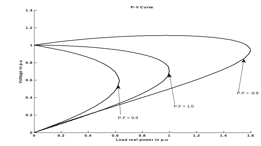
The above equations can give P-V curve when the values of V1 , β, and X are fixed. As

we changing P, real power load, we will get two voltage solutions at each loading case. But at P=Pmax the voltage solutions we got are of same value and this voltage is called as critical voltage. If P is increased beyond Pmax then the solution will become unsolvable which will indicate voltage collapse. The P-V curves for V1 =1 0, X=0.4 p.u and for different power factor

(25)

16

Figure 2.2 P-V Curve

2.2.2.2 V-Q Curve Analysis

V-Q curves plot voltage at a test or critical bus versus reactive power on the same bus. V-Q curves will give good insight in to system reactive power capabilities under both normal and contingency conditions. The V-Q curves have many advantages. V-Q curves will give reactive power margin at a test bus. Reactive power compensation will provide security to voltage stability problems which is determined by plotting reactive power compensations on to V-Q curves. The slope of the V-Q curve will indicate stiffness of the test bus. This method artificially stresses a single bus which should be confirmed by more realistic methods before coming to conclusion.

0 0 .2 0 .4 0 .6 0 .8 1 1 .2 1 .4 1 .6

0 0 .2 0 .4 0 .6 0 .8 1 1 .2 1 .4

V

o

lta

g

e

i

n

p

.u

Loa d re a l powe r in p.u P - V C urve

P.F = 0.9

P.F = 1.0

(26)

17

2.2.2.3 V-Q Sensitivity Analysis

The V-Q sensitivity analysis will give information regarding the sensitivity of a bus voltage with respect to the reactive power consumption. This analysis can provide system wide voltage stability related information and can also identify areas that have potential problems. The linearized steady state power systems equations can be expressed as

(2.10)

Where ΔP= incremental change in bus real power

ΔQ= incremental change in bus reactive power injection ΔV= incremental change in bus voltage magnitude Δθ= incremental change in bus voltage angle.

Here the elements of matrix J (Jacobian matrix) will give the sensitivity between power flow and voltage changes.

The general structure of the system model for voltage stability analysis is similar to that of transient stability analysis. The overall system equations, comprising a set of first-order differential equations may be expressed as,

(2.11)

(27)

18

Rewriting the linear relationship between power and voltage for each device when =0 can be expressed as

(2.12)

Here “d” stands for device.

All the above elements are for a particular device. A11, A12, A21 and A22 represent system

Jacobian elements.

V-Q sensitivity analysis is done by keeping real power P constant and evaluating voltage stability by considering the incremental relationship between Q and V. when ΔP=0 then

(2.13)

Where

(2.14)

JR is called as reduced Jacobian matrix of the system Equation 2.13 can also be written as

_(2.15)

Where JR-1 is the inverse of the reduced V-Q Jacobian and its ith diagonal element will provide

V-Q sensitivity at bus i.

(28)

19

of the nonlinear nature of V-Q relationship, the magnitudes of the sensitivities for different system conditions do not provide a direct measure of the relative degree of stability.

2.2.2.4 Q-V Modal Analysis

Eigen values and Eigen vectors of reduced Jacobian matrix JR will be useful in describing

voltage stability characteristics.

Let us consider (2.16) Where R= right Eigen vector matrix of JR

L= left Eigen vector matrix of JR

Λ=Diagonal Eigen value matrix of JR

Using modal transformation Equation 2.16 can be written as

_(2.17)

From Equation (2.13)

_(2.18)

(2.19)

Here ri is the ith column right Eigen vector and li is the ith row left Eigen vector. Eigen

value λi and corresponding ri and li define ith mode of Q-V response. Note that

_(2.20)

(29)

20

_(2.21)

_(2.22)

Where is vector of modal volatge analysis and is vector of modal reactive power variations.

From equation (2.22)

(2.23) And Λ-1

is diagonal matrix. Details of development of Equation 2.13 to 2.22 in [1].

From above equations it is clear that if then voltage and reactive power of ith mode are along same direction which implies that voltage stable. If voltage and reactive power of ith mode are along opposite direction which implies voltage unstable. Magnitude of λi

determines degree of stability of ith modal voltage. The smaller the magnitude of positive λi

means ith mode is closer to voltage instability and vice versa. If λi=0 it means that ith modal

voltage collapses.

2.2.2.5 Dynamic Analysis

Dynamic analysis of voltage stability will be same as transient stability because structure for dynamic analysis is going to be the same as transient stability structure. The whole system representation can be done with a set of first order algebraic equations and those equations are and

(30)

21

With initial conditions (X0, V0)

X= State vector of the system V=Bus voltage vector

I= Current injection vector

YN= Network node admittance matrix

By including the action of transformer tap changers and phase shift angle control devices, elements of YN change with bus voltage and time. Because of the time dependent nature of YN,

current injection vector I also becomes time dependent in all equations representing the whole system. These equations can be solved in time-domain by any of the numerical integration techniques and network power flow analysis methods. These techniques take several minutes depending upon the computer speed. By including slower system dynamics which lead to voltage collapse will increase the stiffness of differential equations representing system as we compared to transient stability model. These kinds of differential equations can be solved by implicit integration methods.

2.3 Rotor Angle Stability

According to P. Kundur [1] rotor angle stability is the ability of connected synchronous machine power system to remain in synchronism. This stability mainly concentrates on rotor angle oscillations of the synchronous machine as the power output changes.

(31)

22

(SMIB). This circuit represented by Figure 2.3 has two buses connected by two transmission lines of reactance X1 and X2.

Figure 2.3 Single machine infinite bus system

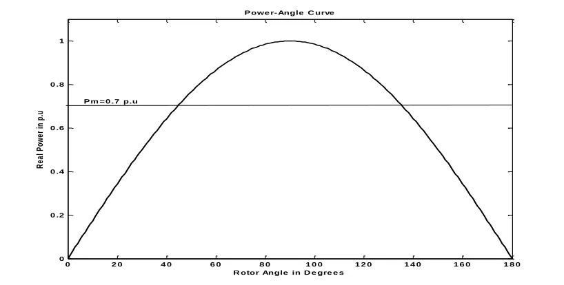
Here the power transferred from generator to infinite bus is a function of angular separation between the rotor of a machine and the infinite bus voltage angle. Neglecting transmission line losses, the relationship between real power and swing angle is

(2.25)

Where XT = XG + X1||X2

(32)

23

Figure 2.4 Power-Angle curve

By considering in plot of Figure 2.4, it is seen that, power transferred will be zero when rotor angle is zero, it increases to maximum as the δ increases up to 900 and a further increase in δ results in decrease in power transfer. For more than one machine systems their relative angle displacement affects the interchange of power in a similar manner.

The rotor angle stability of a system can be divided in two categories of small signal stability and transient stability.

2.3.1 Small Signal Stability

This is also called as small disturbance stability which is the ability of power system to maintain synchronism under small disturbances. These disturbances are originated from small variations in loads and generation. The instability which may be resulted from these variations will lead to two forms, one is steady increase in rotor angle due to lack of synchronizing torque and second one is rotor oscillations of increasing amplitude due to lack of sufficient damping

0 2 0 4 0 6 0 8 0 1 0 0 1 2 0 1 4 0 1 6 0 1 8 0

0 0 .2 0 .4 0 .6 0 .8 1

P owe r- Angle C urve

R otor Angle in D e gre e s

R

ea

l P

ow

er

in

p

.u

(33)

24

torque. Small signal stability depends on initial operating conditions, Strength of transmission system and type of generation excitation controls.

2.3.2 Transient Stability

Transient stability is the ability of power system to maintain synchronism when subjected to severe transient disturbances [1]. This stability depends on both the initial conditions and initial operating state of the system and the severity of the disturbance. For the severe faults in transient stability the system state is altered so that the post disturbance steady state operation differs from the pre fault state. In interconnected large power systems transient instability may not occur in first swing because it may be the result of the superposition of several methods of oscillations. Transient stability studies will be done for 3 to 5 seconds following a disturbance. Sometimes it may be extended to 10 seconds for large systems.

By using the small system which is SMIB considered earlier to describe the transient stability. For simplicity generator is represented by the classical model and the speed governor effects are neglected. Generator voltage behind the transient reactance Xd| is denoted by E|. Rotor

angle δ represents the leading angle between E|

and EB. When a disturbance occurs on the system

then E| remains constant but δ changes as the rotor speed deviates from synchronous speed w0.

The generation equation of motion which is also called as swing equation will be

(2.26)

Pm = mechanical power

(34)

25

2.3.3 Methods of Transient stability analysis

2.3.3.1 Equal Area Criterion

Equal area criterion can determine the transient stability of a system without solving for swing equation. This technique will calculate the information needed for transient stability arrangement from the power angle curve. Equal area criterion requires following relations [1].

(2.27)

(2.28)

(2.29)

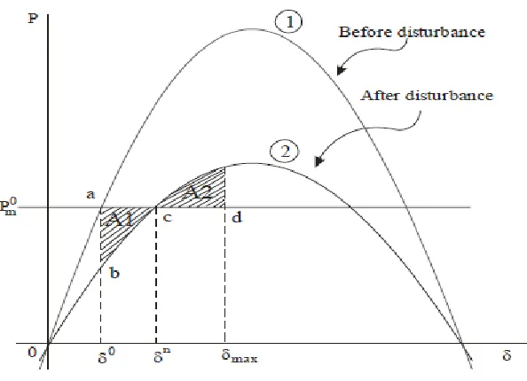
P-δ curve for the system described earlier is shown Figure 2.5.

(35)

26

Curve (1) represents a pre disturbance situation and Pm0 is the mechanical input power to the

generator in steady state and equal to Pe in steady state. It is assumed that constant mechanical

input power, damping is neglected, and classical machine model.

According to the assumption of constant mechanical input power to the generator will be Pm0through out the transient and post disturbance. Point „a‟ in figure 2.5 represents the steady

state operating point and is the steady state rotor angle of the system.

If a fault occurs on one of the transmission line and assume that the line has been disconnected by protective elements in the system then, for one of the line outage impedance of power flow path increases and the maximum power transfer capability decreases which can be realized from the below equation.

(2.30)

Curve 2 in the figure 2.5 reflects the one line outage case for the considered system. Point „b‟ is the operating point for the one line outage case. But the rotor angle cannot change instantaneously because of moment of inertia of the rotor. Now for line outage case Pm is greater

than Pe which is point „b‟ on curve 2. Rotor will accelerate until the operating point reaches point

„c‟ on curve 2. At this operating point rotor angle is δn

and Pm= Pe. But here the rotor speed

higher than synchronous speed, hence rotor angle continues to increase. But for rotor angle greater than δn

, electric power Pe is greater than Pm and the rotor tries to decelerate. At point „d‟

on curve 2 rotor attains its synchronous speed ω0. But still Pe is greater than Pm so that rotor

continues to decelerate and reaches point „b‟. The rotor will oscillate indefinitely about the new equilibrium point δn

(36)

27

The kinetic energy stored in the system when the rotor is accelerating can be shown by the shaded area A1 and this is

(2.31)

The decelerating energy of the system is shown in shaded area A2 and that is

(2.32)

Transient stability will be determined from areas A1 and A2 .

I. When A1 > A2 system is unstable

II. If A1< A2 system is stable

III. For A1=A2 critical angle and critical clearing time can be determined for the system.

2.3.3.2 Numerical Integration Techniques

From the last discussion it can be stated that total power system can be represented as

(2.33)

(37)

28

2.3.3.3 Transient Energy Function Approach

TEF is one of the direct methods to determine the transient stability of a system without solving for different equations. This method uses transient energy to determine the transient stability of the power system. The approach in TEF method for power system is equivalent to a ball rolling on the inner surface of a bowl [39, 40]. Initially consider the power system is operating at stable equilibrium point and it is equivalent to ball resting at the bottom of the bowl. When a fault occurs on the power system then system will accelerate and gains some kinetic energy and it moves away from SEP and it is equivalent to ball moving away from its resting point when some external force is applied on it. After the fault is cleared the kinetic energy gained during fault on period will be converted in to potential energy same as the ball rolling up the potential energy surface. The system has to absorb the kinetic energy to avoid instability because this kinetic energy will try to bring the generators towards a new equilibrium point which is unstable. This potential energy absorbing capabilities depends on post disturbance system. Transient energy function method can be explained well with the figure (2.6).

(38)

29

The curve represents potential energy of the system. Area A1 is the kinetic energy gained

when the system is having a fault and δc is the fault clearing rotor angle. Area A2 is the total

energy present in the system at clearing angle δcl. If the post fault system can convert the

excessive kinetic energy then the system is said to be stable that is kinetic energy at clearing time plus the potential energy clearing time is less than the potential energy of a unstable equilibrium point. This can be shown in equation form as

(2.34)

If the above condition does not satisfy then the system is unstable.

2.4 Unification of Voltage and Angle Stability

As mentioned in chapter 1, this research is continuation of research done by Dr. Sze Mei Wong and Dr. Parviz Rastgoufard at Tulane University on “Unification of Angle and Magnitude Stability to Investigate Voltage Stability of Large-Scale Power System”. This part of the chapter will give some detailed idea on unification approach and how it is used to predict voltage stability from angle stability of a power system.

Dynamic systems with multiple time scales arise naturally in many domains. Here we are interested in system of Differential equations in Rm+n of the form

(2.35)

(39)

30

These systems are called singularly perturbed differential equations or fast slow vector fields [26]. Here ε ≥ 0 is a small parameter, x variables are called as fast variables, y variables are called as slow variables, and these two systems have time variables t and T with dT/dt=ε.

A power system is highly nonlinear system and is dynamic. Power system stability problems can be modeled as a fast-slow nonlinear system due to interaction of mechanical and electrical time constant. If a power system is represented by Equation (2.34), Equation (2.35) then x stands for the state variables of the system and those are rotor angles and rotor speed, y represents algebraic variables which are slow and those are bus voltage magnitudes and voltage angles. P is the parametric variables like real and reactive power injections at each bus [38].

If ε0 the which means y becomes a constant value,

(2.37)

Equation 2.37 resembles the differential equation used for transient stability studies while changes of the algebraic variables y are neglected. Solving function f gives equilibrium points of transient response of the system under different loading conditions. The transient solutions are Xtp1, Xtp2,…., Xtpmax and any value larger than Pmax result in transient unstable. Here “t” stands

for transient solution. By linearizing the differential equation it will become as where A is system matrix. If all the eigenvalues of the A matrix have negative real parts, the system is considered as transient stable.

When , g(x,y,p)=0 and x becomes as constant value.

(40)

31

Above equation represents the steady state response of a power system. By solving the above equation we will get steady state value of the variable vector and the solution under different loading conditions can be expressed as Xvp1, Xvp2,…., Xvpmax. Linearizing the function g

algebraic equation will become as,

(2.39)

Where J is the unreduced Jacobian matrix,

If all the Eigen values of J are negative then the system is considered as voltage stable.

There is a correlation between the solutions from transient stability and that of voltage stability [38]. Form eq (2.36) which represents transient stability, by setting indicates dynamcis have vanished and system reached its equilibrium state. This can be represented by set of non linear algebraic equations

(2.40)

And for a specific equilibrium point

(2.41)

xeq, yss and pss are variables from transient stability and they can be obtained in less than a

minute, while xa, ya and pa are variables from voltage stability and it usually takes 30 minutes to

obtain them. If Xeq can predict xa, yss can predict ya and pss can predict pa then 30 minutes result

(41)

32

2.5 Pattern Recognition

According to Duda and Hart [41], “pattern recognition is act of taking in raw data and taking an action based on the category of the pattern”. A pattern is a type of reoccurring event or object which can be named. Finger print image, hand written word, speech, etc can be considered as a pattern. The process of recognition is a machine classification and assigns the given objects to prescribed classes. Figure (2.7) illustrates the flow chart pattern recognition model development and data classification.

Pattern recognition techniques are used in engineering applications like wave form classification where wave forms corresponding to one class of data are discriminated from the data corresponding to a different class. We are using pattern recognition techniques to distinguish voltage stable waveforms from voltage unstable waveforms. Regularized least-squares (RLS) classification is used for our binary classification problem. RLS is a learning method that obtains solutions for binary classification problems.

(42)

33

Physical Environment

Data Acquisition/Sensing

Pre Processing

Feature Extraction

Features

Classification

Post-Processing

Decision

Training Data

Pre Processing

Feature Extraction/Selection

Features

Model Learning/Estimation Model

Figure 2.7 Flow Chart of Pattern Recognition Model [38]

2.5.1 Regularized Least-Square Classification (RLSC)

As mentioned earlier RLSC is a learning method that obtains solution for binary classification via Tikhonov regularization in a Reproducing Kernel Hilbert Space using the square loss function [42-43]. Let‟s assume X and Y are two sets of random variables and training set for pattern classification is S = (x1, y1), …., (xn, yn) and it satisfies and for

all i. the main goal is to learn a function f(x) while minimizing the probability of error described by Equation 2.42.

(2.42)

(43)

34

(2.43)

Above problem is ill defined, because the set of functions required in minimizing Equation 2.43 are not considered. By representing function f lie in a bounded convex subset of a Reproducing Kernal Hibert Space H that simultaneously has small empirical error and small norm in reproducing Kernel Space generated by kernel function K. The resulting minimization problem can be solved via Lagrange multipliers.

(2.44)

Whereas is the norm in the hypothesis space defined by kernel k.

The solution for Tikhonov regularization problem can be solved by Representer Theorem [48, 49] and it is:

(2.45)

Learning algorithm for this problem is very simple. First kernel matrix K is constructed from training set S.

Next step is to compute the vector coefficients c= (c1,c2, …., cn)T by solving the system of

linear equations

(2.46)

(44)

35

Where y= (y1, …., yn)T and I is the identity matrix of dimension n and finally classifier is,

(2.48)

(45)

36

Chapter 3 HYPERSIM and EMTP-RV

This chapter will explain about HYPERSIM and EMTP-RV environment and in build models and hardware structure of Hypersim and EMTP-RV.

3.1 Introduction to HYPERSIM real time simulator

HYPERSIM is fully digitalized real time power system simulator. It can simulate various kinds of power system networks to study about the dynamic stability and electromagnetic transients. Hypersim has large number of in-built models (Libraries), like synchronous machines, motors, different types of loads, control equipment like breakers, HVDC and SVC. Its hardware is designed by SGI and the software is by Hydro-Quebac Research Institute (IREQ).

(46)

37

3.1.1 HYPERSIM Hardware Environment

Hypersim‟s hardware environment requires two types of different platforms to execute power system networks. One is HYPERSIM WORKSTATION and the other one is

HYPERSIM REAL TIME COMPUTATION ENGINE.

Hypersim workstation is a computer which can interact with the simulator. It can be one of two types from the below mentioned workstation types.

i. Standard PC based on Linux Redhat 7.2/7.3 ii. Sun workstation based on UNIX Solaris 5.6/5.8

Hypersim Real time computation engine is a parallel processing simulator and is one of the two types and each of them has their own advantages and disadvantages.

i. SGI super computer (family of 2000, 3000, 300). ii. PC cluster ( A group of standard Intel processors).

3.1.2 HYPERSIM Software Environment

Hypersim software consists of many tools for the real time simulation and real equipment tests and they are

HYPERSIM: It is a graphical interface to edit and control the power systems to simulate. HYPERVIEW: This is a GUI tool for Netlist, Load flow and Snapshot.

(47)

38

HYMONITOR: This will monitor the performance of parallel processors. TESTVIEW: Testview is for automatic control and testing of the simulator. SI5: This one is a database to store all types of results.

3.2 EMTP-RV

(48)

39

3.3 Power system components in HYPERSIM and EMTP

As mentioned this chapter is going to discuss about the Hypersim and EMTP in building power system models. The models we are going to discuss will represent the generalized models for Hypersim and EMTP. We are going to discuss about synchronous generators, excitation system, stabilizer, transmission lines, transformers, loads especially dynamic loads. This discussion will be started with generator section.

3.3.1 Synchronous Generator

The synchronous generator model in Hypersim is implemented by the Park‟s (DQ) equations using sletz‟s method [44]. There are two equations and one is D-axis equation and other one is Q-axis equation. The block diagrams for D and Q axis are shown below and the parameters in the block diagram are explained after the diagram. These parameters will be the same for EMTP.

(49)

40

Figure 3.2 Generator Q-axis Block diagram [44] X1-Armature leakage Reactance

Ra-Armature resistance

Xd-Direct synchronous reactance

Xd‟-Direct transient reactance

Xd”-Direct sub-transient reactance

Xq-Quadrature synchronous reactance

Xq‟-Quadrature transient Reactance

Xq ”

-Quadrature sub-transient reactance Td0‟-Direct axis transient time constant

Td0”- Direct axis sub-transient time constant

Tq0‟- Quadrature axis transient time constant

Tq0”- Quadrature axis sub-transient time constant

(50)

41

to have required terminal voltage at the generator terminals. To calculate these values it requires Active and reactive power references.

Synchronous generator control panel has one more section for load flow values. It will ask for type of bus that is slack or generator bus, voltage magnitude, voltage angel, active power and reactive power limits. If the generator is connected to a slack bus then the active power delivered by the generator is calculated by load flow solution and voltage angle is zero (reference bus).

3.3.2 Excitation System

Excitation system controls the terminal voltage of a synchronous machine. This will allow regulating the voltage at terminals of machine or on the high side of step up transformer. This regulation is done by varying the field voltage of the synchronous machine. That is based on the difference between the desired reference voltage and the actual voltage at the terminal at that particular instant. Excitation system consists of two sections one is excitation and other one is regulating system. Excitation system block diagram is given below and the parameters in the block diagram are explained after that.

Efd Vin

T K

a a

S



1 T

T

b c

S S

 

1 1

T K

f f

S S



1

Vimax

Vimin

Error Limiter

Feedback

Filter Regulation and Exec_Limiter Efd_min

Efd_max Vf

-Ve

+

(51)

42

Vin-Control input

Ve-Control error

Vf-Feedback voltage

Efd-Field voltage

Ta-Time constant of regulator

Tb-Time constant (lead) of transient filter

Tc-Time constant (lag) of transient filter

Ka-Gain of regulator

Kf-Gain of feedback

Vimin, Vimax-Loop error limits

Efd_min, Efd_max-Execitation voltage limits

From the block diagram it can be observed that excitation voltage to the exciter field of the generator is limited between Efd_min and Efd_max.

3.3.3 Stabilizer

This system is mainly designed to damp the electromagnetic oscillations. The output of the stabilizer is given to excitation system so that it can control the field voltage at the time of transients. Inputs for stabilizer are Pe or Pef (filtered electric power) and gate opening signal.

Here Pe is for steam turbine and is the electric power with no filtering and Pef is for hydraulic

machine and is the electric power with filtering. Block diagram for the stabilizer is given below and the parameters are explained later.

T

K

S S S 5 5 1

T

S ₆ 1 1

 1 S_A₁ _S2_A₂

1



 S_TT

S 2 1 1 1   T T S S 4 3 1 1   Vst_max Vst_min Vsi Vst

(52)

43

3.3.4 Transmission lines:

Hypersim and EMTP consist of different types of transmission lines like frequency constant distributed parameter lines and Pi lines. Pi lines are mainly used for short length transmission lines. Both types of transmission lines have coupled lines. All of these different types of transmission lines ask for same common parameters like length of transmission line, RLC parameters distribution type that is transposed or un-transposed, transformation matrix and RLC values for different sequences i.e positive, negative and zero sequence.

If the line is a transposed line then Hypersim and EMTP will take its own inbuilt transformation matrix but if the line is an un-transposed line then user has to give transformation matrix Ti values. If the line is a transposed line then negative sequence parameters values will

cancel out and it won‟t ask for those parameters. These softwares will ask in such a way that 0, 1, 1 modes which means zero, positive, positive. If it is a un-transposed line then modes for RLC is named as 1, 2, 3 which is mean by zero, positive, negative. All the zero, positive and negative sequence values required have to mentioned in per unit if user selects per unit system in the control panel of transmission line. Hypersim can also accept EMTP(.PUN) file as input instead of transformation matrix and RLC parameter values.

This thesis test system is using single frequency constant distributed parameter lines and Pi lines. All the transmission lines are assumed as transposed lines.

3.3.5 Loads

(53)

44

(54)

45

Chapter 4 Test System

4.1 IEEE 39 Bus Test system:

The IEEE 39 BUS (NEW ENGLAND) equivalent power system is used to study the voltage stability dynamics. This test system has a total of 39 buses of which 10 buses are generator buses and this system has a total of 19 loads at different buses. IEEE 39 BUS system also consists of 12 transformers, 10 generators and 34 transmission lines. This system is shown in figure (4.1). This chapter will give the information about the test system in a form that HYPERSIM and EMTP can accept the data.

(55)

46

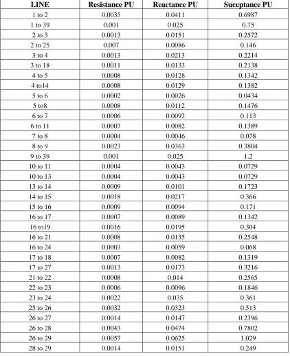
4.2 Transmission Lines

Table 4.1 Transmission line data

LINE Resistance PU Reactance PU Suceptance PU

1 to 2 0.0035 0.0411 0.6987

1 to 39 0.001 0.025 0.75

2 to 3 0.0013 0.0151 0.2572

2 to 25 0.007 0.0086 0.146

3 to 4 0.0013 0.0213 0.2214

3 to 18 0.0011 0.0133 0.2138

4 to 5 0.0008 0.0128 0.1342

4 to14 0.0008 0.0129 0.1382

5 to 6 0.0002 0.0026 0.0434

5 to8 0.0008 0.0112 0.1476

6 to 7 0.0006 0.0092 0.113

6 to 11 0.0007 0.0082 0.1389

7 to 8 0.0004 0.0046 0.078

8 to 9 0.0023 0.0363 0.3804

9 to 39 0.001 0.025 1.2

10 to 11 0.0004 0.0043 0.0729

10 to 13 0.0004 0.0043 0.0729

13 to 14 0.0009 0.0101 0.1723

14 to 15 0.0018 0.0217 0.366

15 to 16 0.0009 0.0094 0.171

16 to 17 0.0007 0.0089 0.1342

16 to19 0.0016 0.0195 0.304

16 to 21 0.0008 0.0135 0.2548

16 to 24 0.0003 0.0059 0.068

17 to 18 0.0007 0.0082 0.1319

17 to 27 0.0013 0.0173 0.3216

21 to 22 0.0008 0.014 0.2565

22 to 23 0.0006 0.0096 0.1846

23 to 24 0.0022 0.035 0.361

25 to 26 0.0032 0.0323 0.513

26 to 27 0.0014 0.0147 0.2396

26 to 28 0.0043 0.0474 0.7802

26 to 29 0.0057 0.0625 1.029

28 to 29 0.0014 0.0151 0.249

(56)

47

continued.

length of transmission lines however HYPERSIM and EMTP will only accept the per Kilometer or per unit length data for the transmission lines. For that reason we need the transmission lines length. We cannot directly assume the length [1]. Phase constant β is practically the same for all transmission lines and this is because of propagation velocity which is somewhat slower than the light velocity (3,00,000 Km/s) i.e

. We calculated the length of each line depending upon the

wave propagation velocity and values are given below.

Table 4.2 Transmission line data for HYPERSIM

LINE Length(Km) R per Km PU

Reac per Km PU

Suc PER Km PU

1 to 2 133.295 2.62575E-05 0.000308339 0.005241756

1 to 39 108 9.25926E-06 0.000231481 0.006944444

2 to 3 48.97214 2.65457E-05 0.000308339 0.005251966

2 to 25 27.89142 0.000250973 0.000308339 0.005234585

3 to 4 54 2.40741E-05 0.000394444 0.0041

3 to 18 42 2.61905E-05 0.000316667 0.005090476

4 to 5 32 0.000025 0.0004 0.00419375

4 to14 33 2.42424E-05 0.000390909 0.004187879

5 to 6 8.432289 2.37184E-05 0.000308339 0.005146883

5 to8 32 0.000025 0.00035 0.0046125

6 to 7 25 0.000024 0.000368 0.00452

6 to 11 26.59414 2.63216E-05 0.000308339 0.005222955

7 to 8 14.91866 2.68121E-05 0.000308339 0.00522835

8 to 9 93 2.47312E-05 0.000390323 0.004090323

9 to 39 135 7.40741E-06 0.000185185 0.008888889

10 to 11 13.94571 2.86827E-05 0.000308339 0.005227415

10 to 13 13.94571 2.86827E-05 0.000308339 0.005227415

13 to 14 32.7562 2.74757E-05 0.000308339 0.005260073

14 to 15 70.37718 2.55765E-05 0.000308339 0.005200549

15 to 16 31.5 2.85714E-05 0.000298413 0.005428571

16 to 17 27 2.59259E-05 0.00032963 0.00497037

16 to19 60 2.66667E-05 0.000325 0.005066667

16 to 21 46 1.73913E-05 0.000293478 0.00553913

16 to 24 15.5 1.93548E-05 0.000380645 0.004387097

(57)

48 Table 4.2 continued.

23 to 24 87 2.52874E-05 0.000402299 0.004149425

25 to 26 100 0.000032 0.000323 0.00513

26 to 27 46 3.04348E-05 0.000319565 0.005208696

26 to 28 150 2.86667E-05 0.000316 0.005201333

26 to 29 200 0.0000285 0.0003125 0.005145

28 to 29 47.5 2.94737E-05 0.000317895 0.005242105

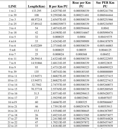
4.3 Transformers

Transformers details for this test system are taken from [N]. Those details consists of RT

(Resistance) and XT (Reactance) which are equivalent resistance and reactance referred with

respect to primary or secondary. For this system we assumed that the values are with respect to primary winding of the transformer. Transformer details are given in the below table.

Table 4.3 Transformers data

BUS BUS RESISTANCE(RT)

REACTANCE(XT)

30 2 0.0000 0.0181

37 25 0.0006 0.0232

31 6 0.0000 0.0250

32 10 0.0000 0.0200

11 12 0.0016 0.0435

13 12 0.0016 0.0435

34 20 0.0009 0.0180

20 19 0.0007 0.0138

33 19 0.0007 0.0142

36 23 0.0005 0.0272

35 22 0.0000 0.0143

38 29 0.0008 0.0156

(58)

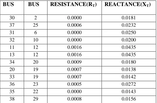
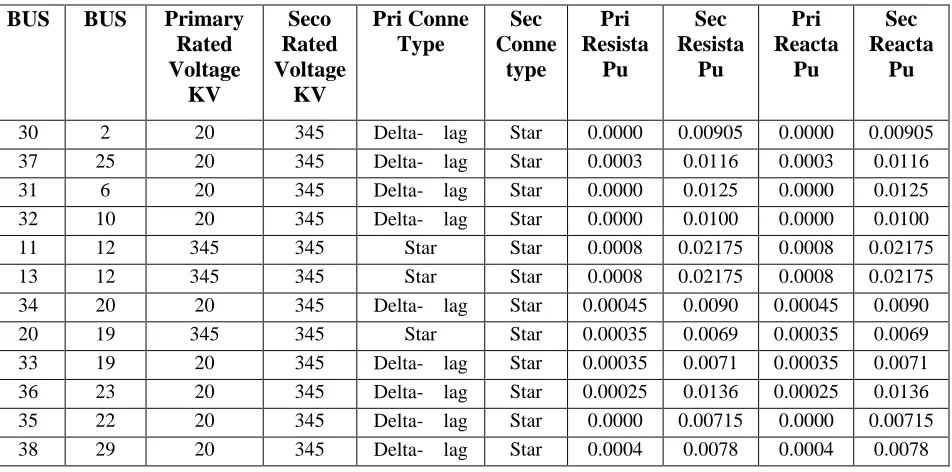
49

with rated voltage of 345KV. All the remaining transformers are grounded stat-star with both the windings rated at 345KV.

But HYPERSIM will ask for individual winding data. As from [46].

X1=X2/K2=X01/2 (4.1)

Where K is turns ratio, X01 total equivalent reactance and X1, X2 are primary, secondary

windings individual reactances. Above statement is based on a assumption that the transformers are well designed.

Below table will give all the details regarding transformers for HYPERSIM and EMTP model. All the per unit values of transformers are taken at 100MVA base.

Table 4.4 Transformers data for HYPERSIM

BUS BUS Primary

Rated Voltage

KV

Seco Rated Voltage

KV

Pri Conne Type

Sec Conne

type

Pri Resista

Pu

Sec Resista

Pu

Pri Reacta

Pu

Sec Reacta

Pu

30 2 20 345 Delta- lag Star 0.0000 0.00905 0.0000 0.00905 37 25 20 345 Delta- lag Star 0.0003 0.0116 0.0003 0.0116

31 6 20 345 Delta- lag Star 0.0000 0.0125 0.0000 0.0125

32 10 20 345 Delta- lag Star 0.0000 0.0100 0.0000 0.0100 11 12 345 345 Star Star 0.0008 0.02175 0.0008 0.02175

13 12 345 345 Star Star 0.0008 0.02175 0.0008 0.02175 34 20 20 345 Delta- lag Star 0.00045 0.0090 0.00045 0.0090

20 19 345 345 Star Star 0.00035 0.0069 0.00035 0.0069

(59)

50

4.4 Generators

IEEE 39BUS system has 10 generators at different buses which were already mentioned. Out of those 10 generators a generator at BUS 31 which is named as GEN2 is assumed as a slack bus generator. Except BUS31 all the buses numbered as 30 to 39 are called as PV buses because of the generators connected at those buses. All the remaining buses are called as PQ buses. The bus which is considered as slack bus has a voltage angle as zero because all the remaining voltage angles are measured with respect to the slack generator. The generator which is considered as slack generator will give all the deficient power in the network and it also gives the power required to cover the losses.

Below table gives the information regarding initial load flow conditions for IEEE 39 BUS 10 generators. All the values are in 100-MVA power base and machines rated terminal voltage.

Table 4.5: Generators initial load flow details

BUS GENERATOR RATED

VOLTAGE KV

VOLTAGE

Pu

ACTIVE POWER

Pu

30 10 20 1.0475 2.50

31 2 20 0.9820 Slack Generator

32 3 20 0.9831 6.50

33 4 20 0.9972 6.32

34 5 20 1.0123 5.08

35 6 20 1.0493 6.50

36 7 20 1.0635 5.60

37 8 20 1.0278 5.40

38 9 20 1.0265 8.30

39 1 345 1.0300 10.0

Pattern Recognition of Power Systems Voltage Stability Using Real Time Simulations

ScholarWorks@UNO

ScholarWorks@UNO

Pattern Recognition of Power Systems Voltage Stability Using

Pattern Recognition of Power Systems Voltage Stability Using

Real Time Simulations

Real Time Simulations

Acknowledgements

Table of Contents

List of Tables

List of Figures

Abstract

Chapter 1

Introduction

1.1 A Review of Voltage Stability

1.2 Review of Static Analysis Methods of Voltage Stability

:

1.3 Review of Dynamic Analysis Methods of Voltage Stability:

1.4 Historical Review of Major Blackouts

Chapter 2

Background and Mathematical Model

2.1 Voltage stability and Transient stability:

2.2 Voltage Stability:

2.3 Rotor Angle Stability

2.4 Unification of Voltage and Angle Stability

2.5 Pattern Recognition

Chapter 3

HYPERSIM and EMTP-RV

3.1 Introduction to HYPERSIM real time simulator

3.2 EMTP-RV

3.3 Power system components in HYPERSIM and EMTP

T

T

K

T

Chapter 4

Test System

4.1 IEEE 39 Bus Test system:

4.2 Transmission Lines

4.3 Transformers

4.4 Generators