Volume 7 - Article 14 | Pages 499–522

(1)

Research Article

Algorithm for decomposition of differences between

aggregate demographic measures and its application to life

expectancies, healthy life expectancies, parity-progression ratios and

total fertility rates.

Evgueni M. Andreev1 Vladimir M. Shkolnikov2

Alexander Z. Begun3

Abstract

A general algorithm for the decomposition of differences between two values of an aggregate demographic measure in respect to age and other dimensions is proposed. It assumes that the aggregate measure is computed from similar matrices of discrete demographic data for two populations under comparison. The algorithm estimates the effects of replacement for each elementary cell of one matrix by respective cell of another matrix. Application of the algorithm easily leads to the known formula for the age-decomposition of differences between two life expectancies. It also allows to develop new formulae for differences between healthy life expectancies. In the latter case, each age-component is split further into effects of mortality and effects of health. The application of the algorithm enables a numerical decomposition of the differences between total fertility rates and between parity progression ratios by age of the mother and parity. Empirical examples are based on mortality data from the USA, the UK, West Germany, and Poland and on fertility data from Russia.

1 _{Institute for Prognosis of the National Economy, Centre of Demography and Human Ecology,}

Nakhimovsky prosp., 47, 117418, Moscow; E-mail: [email protected]

2 _{Max Planck Institute for Demographic Research, Doberaner Str. 114, D-18057 Rostock, Germany.}

E-mail: [email protected]

3 _{Universität der Bundeswehr Hamburg, Holstenhofweg 85, 22043 Hamburg;}

(2)

1. Introduction

In the 1980s, interest in decomposition appeared in relation to the particular problem of the decomposition of differences between two life expectancies. Nowadays, researchers are trying to develop general approaches which would solve the decomposition problem for wider classes of demographic measures (Das Gupta, 1994, Das Gupta, 1999, Vaupel and Canudas Romo, 2002, Shkolnikov, Andreev and Begun, 2001). The present study contributes to this line of research.

A variety of aggregate measures can be computed from demographic tables. Each of them aggregates a vector or a matrix of elementary rates of demographic events into one number. When analyzing changes in an aggregate demographic measure in time or its variations across countries, it is useful to be able to decompose observed changes or differences by age and other demographic dimensions such as birth order, cause of death, or population group. Decomposition aims at estimating contributions of differences between elementary rates of demographic events to the overall difference between two values of the aggregate measure.

This task is easier when analyzing for differences between two linear aggregates of elementary rates like two age-standardized rates or two total fertility rates. However, some of the aggregate measures are linked to elementary rates in a complex way. For example, life expectancy at birth is a functional of the vector of age-specific death rates, which has to be computed by complex acccumulation of these rates by means of the life table. The conventionalTFR is simply the sum of age-specific fertility rates. However,

TFR computed from age- and parity-specific fertility rates (denoted hereafter as

TFR_P) is a complex measure, which has to be computed by means of the parity progression table.

A discrete method for decomposition of a difference between two life expectancies was independently developed in the 1980s by three different researchers from Russia, the USA, and France (Andreev, 1982, Arriaga, 1984, Pressat, 1985). The formulae for decomposition by Andreev and Pressat are exactly equivalent. Arriaga’s formula is written in a slightly different form, but it is essentially equivalent to the formulae by Andreev and Pressat (Shkolnikov et al., 2001). A continuous version of the method for decomposition of differences between life expectancies by age was developed by Pollard (1982).

It appears that existing formulae for age-decomposition of the difference between life expectancies are just particular forms of a general algorithm, which includes the

(3)

) ( 2 0 2 0 e M e <

respective elements of another matrix. This approach has its roots in the general idea of standardization (Kitagawa, 1964).

The first section of the present paper is devoted to the decomposition of differences between life expectancies and between healthy life expectancies. First, we show how the conventional formula for decomposition of differences between life expectancies derives from the general replacement algorithm. Second, the same approach is applied to the age-decomposition of differences between health expectancies. These measures combine data on mortality with data on health. Each measure is calculated from two independent vectors, that is, of age-specific mortality rates and of the age-specific prevalences of "good" health. Correspondingly, each elementary age-component of the difference between two health expectancies is to be split further into the effects of mortality and of health.

The second section deals with two aggregate measures of fertility based on the parity-progression table, namely parity-progression ratios and the total fertility rate. Both indicators are based on the matrix of elementary fertility rates by age of the mother and parity. We show that the results of an exact decomposition according to the algorithm of stepwise replacement differ from those returned by simpler methods.

In sections 1 we solve the decomposition problems by developing formulae for the components. In section 2 we describe a procedure for their numerical estimation.

2. Decomposition of differences between two life expectancies

and between two healthy life expectancies

Life expectancies

Consider two life expectancies at birth and computed in a conventional way from two vectors of age-specific mortality rates

1 1

x m

M < and 2 2

x

m

M < ,x=0, 1, 2, ...

ϖ

. Transition from life expectancy

e

1₀ to

life expectancy

e

₀2 corresponds to a transformation of vector M1 into vector _M2_. Such a transformation can be completed by a stepwise replacement in an age-by-age mode of the elements of the first vector by respective elements of the second vector.

Let _M[x]_{be the vector, consisting of elementary mortality rates} 2

1my at ages

x

y

;

and 1

1my at ages

y

″

x

(Note 1). The difference 02|x1 <e0(M[x]),e01 ,

χ is a

contribution of ages from

y

;

x

to the overall difference 1 0 2 0 e

e , . Using definitions of the standard life tables functions, it can be presented as

(4)

1 1 2 1 | 0 2 | 0 1 0 ] [ 0 1 2 |

0x,

<

e

(

M

x

)

,

e

<

(

L

x

,

L

x

)

∗

(

l

x

,

l

x

)

√

e

x

χ

, (1)

where

<

〉

x

l

t

dt

L

0 |

0

(

)

. The first additive term in (1) is the length-of-life effect of

replacement 1↑2 at ages under x, the second additive term is the effect of 1↑2 replacement at ages underx on life expectancy after agex.

The contribution of elementary age interval[x,x∗1) can be expressed as

)

(

)

(

[ ] 0 ] 1 [ 0 1 2 | 0 1 2 1 | 0 1

2 x x

x x

x,

<

χ

,∗

,

χ

,

<

e

M

∗

,

e

M

χ

(2)

Formula (2) is a form of the general algorithm of stepwise replacement for a one-dimensional decomposition of a difference between two aggregate measures by age.

Substitution of (2) in (1) yields

)

(

)

(

1 1 2 1 2 1 1 2 2 1 2 ∗ ∗ ∗

,

_<

_,

x x x x x x

x

l

e

l

e

χ

.

Thus, the overall difference between two life expectancies is



< ,

<

,

ϖ

χ

0 1 2 1 0 2 0 x x

e

, (3a)

where

l

_ϖ_∗₁ and

e

_ϖ_∗₁ are assumed to be 0.

In a similar way, one can decompose the difference

e

1₀

,

e

₀2 by making 2↑1 replacements instead of 1↑2 replacements:



< ∗ ∗ ∗

<

,

_<

_,

<

,

ϖ

χ

ϖ 0 2 1 1 1 1 1 2 1 1 0 2 1 2 0 1

0

[

(

)

(

)]

x x x x x x x x

x

l

e

l

e

(5)

(3) Components

χ

_x2,1 are somewhat different from components

,

χ

_x1,2. That is to say that the decomposition of differences between life expectancies depends on the

permutation of vectors under

comparison. Both E.Andreev (1982) and R.Pressat (1985) noticed this important feature. They suggested averaging as a way to obtain symmetrical components i.e.

) (

2

1 ₂_,₁ ₁_,₂ , √

< _x _x

x χ χ

χ .

The latter expression exactly replicates the formulae by E. Andreev (1982) and R. Pressat (1985).

Numerous empirical examples of decompositions of differences between life expectancies can be found elsewhere (Shkolnikov et al., 2001).

Replacement running from young to old ages looks natural and meaningful. Nevertheless, it is not obvious why the replacement algorithm goes this way. Generally speaking, it could be organized differently. For example, it could run from old to young ages (Pollard, 1988) or in a random manner.

The most general procedure for the replacement of one element should include 1

2

ϖ, replacements. For every age x the replacement should be performed with all possible combinations of M1_y and

M

_z2, at ages y andz other than age x. The final

contribution of agex should be calculated as the average of

2

ϖ,1 components.

This procedure is extremely laborious given high numbers of age groups (about 20 for abridged life tables and about 100 for complete ones). Several numerical experiments (not shown here) suggest that results of "complete" decomposition of differences between life expectancies are close to the results returned by formula (3). So, there are reasons to avoid laborious calculations if we agree to follow the existing tradition of making replacements in ascending order of ages. It guarantees consistency regarding the existing formulae for the decomposition of differences between life expectancies by age and, as we show below, allows to develop similar decomposition formulae for the age-decomposition for other aggregate measures such as Gini coefficients or healthy life expectancies.



< ∗ ∗ ∗ ∗ ∗ ∗

< , , , , , , , √ < < , ϖ χ ϖ 0 x 2 1 x 1 1 x 1 1 x 2 x 1 x 1 x 1 1 x 2 1 x 2 1 x 1 x 2 x 2 x 0 x x 1 0 2

0 {[ ( ) ( )] [ ( ) ( )]}

(6)

Health expectancies

Health expectancy indicators can be built in several ways (Cambois, Robine and Brouard, 1999, Robine, Romieu and Cambois, 1999). So far, the "observed prevalence life table method" by D.Sullivan (1964) is the most widely used method. According to this method, health expectancy is defined as

x x x

L

h

ο

ϖ

√

<



<0 1

0 , (4)

where

ο

_x is the share of person-years lived in "good" health within the elementary age interval [x, x+1). Usually the health-weights

ο

_x are obtained from nationally representative surveys including questions on self-perceived health, self-perceived disability, ill-health or physical performance scales (Wilkins and Adams, 1983, Robine, Romieu and Cambois, 1999, Doblhammer and Kityr, 2001, Crimmins and Saito, 2001).

According to (4), two vectors are needed for calculating the health expectancy. These are the vector of age-specific mortality rates

M

and the vector of age-specific health-weights

Ο

. Correspondingly, decomposition of the difference between two health expectancies should include additional splitting of each age-component into effects of mortality and health.

According to the algorithm of stepwise replacement, the component of the overall difference in

h

₀ due to the difference between mortality rates at agex is

)]} , ( ) , ( [( )] , ( ) , ( {[( 2

1 [] [ 1]

0 ] 1 [ ] 1 [ 0 ] [ ] [ 0 ] [ ] 1 [ 0 1

2, _< x∗ _Οx _, x _Οx _∗ x∗ _Οx∗ _, x _Οx∗

x h M h M h M h M

κ (5)

The component of the overall difference in

h

₀ due to the difference in health-weights at agex is

)]} , ( ) , ( [ )] , ( ) , ( {[ 2

1 [ 1] []

0 ] 1 [ ] 1 [ 0 ] [ ] [ 0 ] 1 [ ] [ 0 1

2 x x x x x x x x

x < h M Ο ,h M Ο ∗ h M Ο ,h M Ο

∗ ∗

,

φ (6)

Expressions (5) and (6) allow to estimate components

κ

2_x,1 and

φ

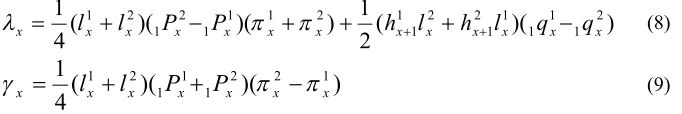
_x2,1 numerically. It is

also possible to develop formulae for them. Let _i

x i x i x

_l

L

P

1

<

(i=1,2). Then formula (4)

(7)

ℎ = ∑

(

) +

+ ℎ

(7)

The first term corresponds to ages younger thanx, the second term corresponds to age [x, x+1) and the third term corresponds to ages older thanx. The second term is equal to the number of person-years in good health lived at age x. It also consists of three components:

l

_x depends on mortality at ages younger than x, ₁

P

_x depends on mortality at agex and

ο

_x depends on the prevalence of good health at agex.

1→2 replacement of mortality rate at agex produces changes in the second and the third terms of (7). 1→2 replacement of health-weight at agex produces change in the second term of (7).

Insertion of (7) in (5) and (6) leads to

)]}

1 (

(

))

1 (

[(

)]

1 (

(

))

1 (

{[(

2

1

1 1 2 1 1 2 1 1 2 2 1 2 1 1 2 2 1 2 1 1 2 1 1 1 1 1 2 2 1 2 1 1 1 2 1 2 1 2 x x x x x x x x x x x x x x x x x x x x x x x x x

q

l

h

P

l

q

l

h

P

l

q

l

h

P

l

q

l

h

P

l

,

∗

,

∗

,

∗

,

∗

<

∗ ∗ ∗ ∗ ,

ο

κ

or

=1₂ − + + ℎ − .

In a similar way the health-related component at agex is

)]

(

)

[

2

1

2 1

1 2 2 2 1 2 1 1 1 2 2 1 1 2 1 2 x x x x x x x x x x x x

x

l

P

ο

l

P

ο

l

P

ο

l

P

ο

φ

,

<

,

∗

,

or

)

)(

(

2

1

2 2 1

1 1 1 2 1 2 x x x x x

x

l

P

ο

φ

,

<

∗

,

The components

κ

2_x,1

,

φ

_x2,1, produced by 1→2 replacement, should be averaged with 2

1 2 1,

_,

,

x x

φ

(8)

)

)(

(

2

1 )

)(

(

4

1

2 1 1 1 1 2 1 2 1 1 2 1 1 1 2 1 2 1 x x x x x x x x x x x x

x

<

l

∗

l

P

,

P

ο

∗

ο

∗

h

∗

l

∗

h

∗

l

q

,

q

κ

(8)

)

)(

(

4

1

2 2 1

1 1 1 2 1 x x x x x x

x

l

P

ο

φ

<

∗

,

(9)

Age-components

κ

_xof the difference between health expectancies derived from (10) are equivalent to age-components of the difference between life expectancies

χ

_x from (3) if 1

_<

2

_<

1

x x

ο

for all agesx=0,1,2, ...,

ϖ

.

The example in Figure 1 shows age-mortality-health-specific components of the difference between female health expectancies at age 20 in West Germany and Poland. Health-weights are calculated from the data on self-perceived health, extracted from the second and third wave of the World Value Surveys (Inglehart et al., 2000). For each five-year age group weights

ο

_x are the sums of the original proportions of women with "fair", "good" and "very good" self-perceived health. For both countries the mortality rates for the year 1995 are used. From these data health expectancies at age 20 are computed for West Germany and Poland and their difference is decomposed by age according to (8) and (9).

Figure 1 suggests that contributions due to differences in self-perceived health are much greater than those due to differences in mortality. Indeed, 7.2 years of the overall difference of 8.9 years are attributable to differences in health. Although the maximum age-specific contributions are produced for ages from 65 to 75, they are very significant as early as at the age of 50.

(9)

Figure 1: Decomposition of the difference between female health expectancies at age 20 between West Germany and Poland for the mid-1990s.

3. Decomposition of differences between two parity progression

ratios and two TFRs computed from age-parity-specific

fertility rates

The general replacement algorithm can be applied to differences between aggregate fertility measures based on parity-progression tables. In this section we apply the general algorithm of stepwise replacement to estimate the age- and parity-specific components of differences between two parity-progression ratios and of differences between two total fertility rates.

-0.2 0.0 0.2 0.4 0.6 0.8 1.0 1.2 1.4 1.6

20

-2

4

25

-2

9

30

-3

4

35

-3

9

40

-4

4

45

-4

9

50

-5

4

55

-5

9

60

-6

4

65

-6

9

70

-7

4

75

-7

9

80

-8

4

85

+

C

o

n

tr

ib

u

ti

o

n

in

y

e

a

rs

Health Mortality

h(20):

(10)

A conventionalTFR based on age-specific fertility rates is adjusted for population age structure but ignores differences between sequences of births. TheTFR_P based on age-parity-specific fertility rates is adjusted both for age and parity. This type of period fertility measure is valuable for analytical purposes (Kohler and Ortega, 2002, Barkalov, 1999, Darsky and Scherbov, 1990).

Let us consider an example of changes in Russian fertility in the first half of the 1990s. The TFR in this country dropped from 2 in 1989 to 1.4 in 1993-94 (Table 1). Table 1 shows also that in these years the difference between theTFR and theTFR_P in Russia increased.

Table 1: Total fertility rates computed without and with data on parity in Russia in 1989-1994.

Year TFR TFR_P

1989 2.01 1.97 1990 1.89 1.87 1991 1.73 1.75 1992 1.55 1.62 1993 1.39 1.45 1994 1.40 1.46

Sources: Andreev and Barkalov, 1999 Goskomstat, 2001

The parity-progression table is a type of a multi-status demographic table based on the matrix

F

<

f

_x_,_par , in which each elementary fertility rate

f

_x_,_par is a ratio of the number of par-order births to the mid-year population of women aged x with par-1 children. In matrix F, ages are presented as rows and birth orders are presented as columns. Age runs across the interval of reproductive ages

Ζ

,α

∴

, while parity varies from 0 to the highest birth orderp.

(11)

The total parity-specific birth numbers are defined as

B

₀

<

l

__,₀

<

1000 forpar=0

and



<

< α



x x par

par b

B _, for par>0, where

b

_x_,_par are age-parity-specific birth numbers

from the parity-progression table.

Two aggregate fertility measures, which will be used for our next decomposition exercises, are the

parity-progression ratio

par par

par

B

a

<

_∗₁

/

(10)

and the total fertility rate

)

....

(

_

₀ ₀ ₀ ₁ ₀ ₁ ₂ ₁

1

0 ,

<

∗

√

<

√

<



p _p

par

B

a

B

P

TFR

(11)

Formulae (10), (11) and Appendix defineaparandTFR_P as functionals of the matrix of elementary fertility ratesF.

At first glance, (10) and (11) suggests that the decompositions of difference between values ofTFR_P in respect to agex or paritypar can be accomplished in a simple way from

b

_x_,_∂ values and

a

_par values, respectively. N.Barkalov (1999) developed a formula for the components of differences between two TFR_P values. This formula corresponds to the stepwise replacement of

a

1_par by

a

2_par in (11) running from lower to higher parities, although the way of its development by the author was different. It appears, however, that

a

_par depends not only on

f

_x_,_par_∗₁, but also on fertility rates of lower parities

f

_x_,_k (k<par+1). We will show later that numerical results of this method of decomposition are somewhat different from the exact results of the general replacement algorithm.

The general replacement algorithm for decomposition of differences between

par

(12)

replacement of the elements of rowx

f

_x1_,_par by elements

f

_x2_,_par begins only after all

elements

f

_y1_,_par are already replaced by the elements

f

_y2_,_par for rowsy<x. Certainly, the replacement could be organized differently with parity being the "first" dimension and age being the "second" one (see section 3).

The effect of replacement of a given element

f

_x1_,_par by

f

_x2_,_par on

a

_par and on

TFR_P should be calculated 2par-1_{times according to the number of different} combinations of

f

_x1_,_k with

f

_x2_,_l in remaining cells of the same rowx (k; p,l; p and

par l

k÷ ÷ ). Finally, the component produced by agex and paritypar in replacement 1↑2 is the average of all 2par-1_effects.

As in section 1, in order to obtain symmetrical components the whole set of replacements should be completed twice in two directions (1↑2 and 2↑1).

Let us consider another example. Data from the Russian census of 1989 and the micro-census of 1994 allow us to estimate the composition of female population by age and parity. These data combined with annual statistics on births by parity and age of the mother allow us to calculate fertility rates by parity (1, 2, ..., 5+) and age of the mother (15, 16, 17, ..., 54). Thus, we have to operate with two matrices (40 x 5) of elementary fertility rates

F

1 and

F

2. Values of the parity progression ratios, computed from the matrices of 1989 and 1994, show a structure of the rapid drop in Russian fertility between 1989 and 1994 (Table 2).

Table 2: Changes in parity progression ratios and in total fertility rate between 1989 and 1994.

Year 1989

1

, par

a

and

a

1994_par_,₁ TFR_P

1989

and TFR_P1994

1 2 3 4 5+

1989 0.948 0.767 0.293 0.269 0.519 1974 1994 0.895 0.530 0.161 0.182 0.317 1464 1994-1989 -0.053 -0.237 -0.132 -0.087 -0.202 -510

Replacement of a single element of matrix

F

1 by the respective element of matrix

F

2 (or vice versa) includes 16 (24_{) calculations of changes in}

par

(13)

TFR_P. For example, replacement of the upper-left element

f

₁₅1_,₁, corresponding to

age 15 and parity 1, by the element

f

₁₅2_,₁ includes replacements of this element in all

possible combinations with rates

f

₁₅1_,_k and

f

₁₅2_,_l in the remaining 4 cells of the same row with k ÷l and k,l⊆[2,3,4,5+]. These calculations return 16 magnitudes of changes in the output measures (

a

_par and TFR_P) produced by the replacements. Finally, the averages of these 16 values should be computed for each

a

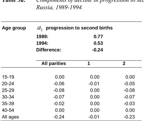
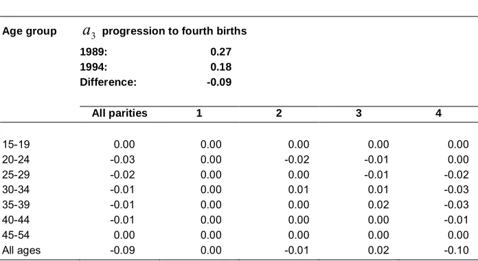
_par and TFR_P.

Tables 3a, 3b, and 3c show age- and parity-specific contributions to the overall changes in

a

₁

,

a

₂and

a

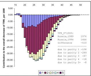
₃in Russia between 1989 and 1994. In general, decreases in progressions to a given paritypar are mostly due to decreases in fertility rates for the same paritypar.However, changing fertility rates at lower parities (par-1 or evenpar -2) also produce some effects on progression to parity par. These effects are more significant for higher parities (e.g. progressions to the third and the fourth births).

Figure 2 shows the structure by age and parity of the decrease inTFR_P in Russia between 1989 and 1994. The greatest contributions are produced by decreases in second births by mothers at ages from 23 to 29.

Table 3a: Components of decline in progression to second births by age and parity, Russia, 1989-1994.

Age group

a

₁ progression to second births 1989: 0.77 1994: 0.53 Difference: -0.24

All parities 1 2

(14)

Table 3b: Components of decline in progression to third births by age and parity, Russia, 1989-1994.

Age group

a

₂progression to third births 1989: 0.29 1994: 0.16 Difference: -0.13

All parities 1 2 3

15-19 0.00 0.00 0.00 0.00 20-24 -0.04 0.00 -0.03 -0.01 25-29 -0.04 0.00 -0.01 -0.03 30-34 -0.03 0.00 0.01 -0.04 35-39 -0.02 0.00 0.01 -0.03 40-54 0.00 0.00 0.00 0.00 All ages -0.13 0.00 -0.02 -0.11

Table 3c: Components of decline in progression to fourth births by age and parity, Russia, 1989-1994.

Age group

a

₃ progression to fourth births 1989: 0.27 1994: 0.18 Difference: -0.09

All parities 1 2 3 4

(15)

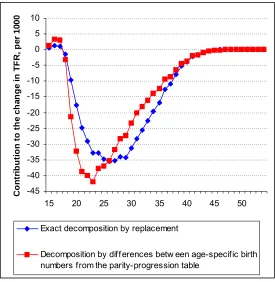
As we mentioned before, formulae (10) and (11) give the impression that decompositions can be made in simpler ways. Indeed, according to (11),TFR_P is the total of all age- and parity-specific birth numbers

b

_x_,_par. Thus, it seems that age-components of the change in TFR_P could be calculated simply as



< <

∂

∂, < ,

p par par x p par par x x

x b b b

b 1 1 , 1 2 , 1 , 2

, . This approach ignores the dependence of i

par x

b

_,

values from fertility rates at parities lower thanpar. The result of such a calculation is substantially biased in comparison to the exact age-components returned by the general replacement algorithm (Figure 3).

Figure 2: Decomposition of decrease in the total fertility rate in Russia in 1989-1994 by age and parity.

-40.00 -35.00 -30.00 -25.00 -20.00 -15.00 -10.00 -5.00 0.00 5.00

15 20 25 30 35 40 45 50

C o n tr ib u ti o n to th e o v e ra ll d e c re a s e o f T R R , p e r 1 0 0 0

1 2 3 4 5

TFR_P*1000:

(16)

Figure 3: Age-components of decrease inTFR_P between 1989 and 1994 in Russia. A comparison of the exact decomposition by the replacement algorithm with a simplified decomposition according to differences in birth numbers from parity progression table.

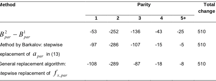
A simplified decomposition of a difference betweenTFR_P values in respect to parity can be accomplished in two different ways. The simplest is to imagine that the par -component of difference between two values ofTFR_P is

B

_par2

,

B

1_par. This approach ignores the dependence of higher-order birth numbers on lower-order births and results in significantly biased parity-components (Table 4). The method by Barkalov, mentioned above, returns thepar-components, which are rather close but not equivalent to exact components returned by the general replacement algorithm. (Table 4).

-45 -40 -35 -30 -25 -20 -15 -10 -5 0 5 10

15 20 25 30 35 40 45 50

C

o

n

tr

ib

u

ti

o

n

to

th

e

c

h

a

n

g

e

in

T

F

R

,

p

e

r

1

0

Exact decomposition by replacement

(17)

Table 4: Components of decline inTFR_P by parity computed by three methods, Russia, 1989-1994 (per 1000)

Method Parity Total

change 1 2 3 4 5+

1 2

par par

B

,

-53 -252 -136 -43 -25 510

Method by Barkalov: stepwise replacement of

a

_par in (13)

-97 -286 -107 -15 -5 510

General replacement algorithm: stepwise replacement of

f

_x_,_par

-108 -289 -87 -18 -8 510

4. Final considerations

The algorithm of stepwise replacement is a universal tool for the decomposition of differences between aggregate measures computed from demographic tables. The number of examples in the present study could be increased. In particular, in an earlier study (Shkolnikov, Andreev and Begun, 2001) we developed a new formulae for the age-decomposition of differences between two Gini coefficients (measures of variability in age at death). In this study we showed also how to decompose the age-components further in respect to age and population composition by social group. Such decomposition can be accomplished by means of the same general algorithm including replacement of age-group-specific death rates and of age-specific population weights of groups.

We would like to add two additional comments regarding two peculiar aspects of the decomposition which were not addressed in sections 1 and 2, but should be kept in mind when making decompositions and interpreting their results.

Path dependence. In the present paper, we always assume that population "jumps" from state 1 to state 2 with no intermediate states in between. However, results of the decomposition could depend on a particular pathway of transition from state 1 to state 2. For example, the age-parity components of change in the RussianTFR_P from 1989 to 1994 are somewhat different from the sums of age-parity components of subsequent transitions 1989↑1990, 1990↑1991, 1991↑1992, 1992↑1993, and 1993↑1994.

(18)

differences between a direct transition (as 1989↑1994) and the sequence of annual transitions are usually small. However, there is no guarantee that such differences would be small in all cases.

Age as a special dimension. In the present paper we treated age as a special dimension in two respects. First, replacement ran from younger to older ages in order to keep a consistency with earlier formulae by Andreev (1982), Arriaga (1984) and Pressat (1985). This approach gives also an opportunity for developing new formulae for other aggregate measures. Second, we were interested in splitting further each age-component according to additional dimensions (effects of mortality and health or effects of parities within each age group). This means that age always played the role of the first dimension. The formulae developed in sections 1 and 2correspond to this particular approach.

(19)

Notes

1. For the sake of simplicity, notation in all formulae of this paper are given for complete demographic tables (tables with single-year age groups). All of them can be easily re-written for abridged demographic tables.

Corrections:

(20)

References

Andreev, E.M. (1982). Metod komponent v analize prodoljitelnosty zjizni. [The method of components in the analysis of length of life].Vestnik Statistiki, 9, 42-47. Andreev, E.M. and Barkalov, N. (1999). Birth tables by sequence of birth. [Tablitsy

rozhdaemosti po ocherednosti rozhdenii.]Voprosy Statistiki, 5, 64-67.

Arriaga, E. (1984). Measuring and explaining the change in life expectancies.

Demography 21(1), 83-96.

Barkalov, N.B. (1999). The fertility decline in Russia, 1989-1996: a view with period parity-progression ratios. Genus, LV(3-4), 11-60.

Cambois, E., Robine, J.-M., Brouard, N. (1999). Life expectancies applied to specific statuses. A history of the indicators and the methods of calculation. Population: An English Selection, 11, 7-34.

Chiang, C.L., Van Den Berg, B.J. (1982). A fertility table for the analysis of human reproduction.Mathematical Biosciences, 62, 237-251.

Crimmins, E.M. and Saito, Y. (2001). Trends in healthy life expectancy in the United States, 1970-1990: gender, racial, and educational differences. Social Science and Medicine, 52, 1629-1641.

Darsky, L.E. and Scherbov, S. (1990). Parity-progression fertility tables for the nationalities of the USSR. IIASA Working Paper, WP-90-53, September. Das Gupta, P. (1994). Standardisation and decomposing of rates from cross-classified

data.Genus, L(3-4), 171-196.

Das Gupta, P. (1999). Decomposing the difference between rates when the rate is a function of factors that are not cross-classified.Genus, LV(1-2), 9-26.

Doblhammer, G. and Kytir, J. (2001). Compression or expansion of morbidity? Trends in healthy-life expectancy in the elderly Austrian population between 1978 and 1998.Social Science and Medicine, 52, 385-391.

Goskomstat (2001).The Demographic Yearbook of Russia. Goskomstat of the Russian Federation, Moscow.

(21)

Inglehart, R., et al. (2000). World Value Surveys and European Value Surveys, 1981-1984, 1990-1993, and 1995-1997. [Computer file]. ICPSR version. Ann Arbor, MI, Inter-University Consortium for Political and Social Research.

Kitagawa, E. (1964). Standardized comparisons in population research.Demography, 1, 296-315.

Kohler H.-P. and Ortega J.A. (2002). Tempo-adjusted period parity-progression measures: assessing the implications of delayed childbearing for cohort fertility in Sweden, the Netherlands and Spain. Demographic Research, 6, article 7, March.

Kohler, H.-P., Billari, F. and Ortega J.A. (2002). Lowest-Low Fertility. Book manuscript.

Lutz, W. (1989). Distributional Aspects of Human Fertility: a Global Comparative Study. New York: Academic Press.

Pollard, J.H. (1982). The expectation of life and its relationship to mortality.Journal of the Institute of Actuaries, 109, Part II, No 442, 225-240.

Pollard, J.H. (1988). On the decomposition of changes in expectation of life and differentials in life expectancy.Demography, 25, 265-276.

Pressat, R. (1985). Contribution des écarts de mortalité par âge à la différance des vies moyennes.Population, 4-5, 766-770.

Robine J.-M., Romieu, I., Cambois, E. (1999). Health expectancy indicators.Bulletin of the World Health Organisation, 77(2), 181-185.

Shkolnikov V.M., Andreev E.M., Begun A.Z. (2001). Gini coefficient as a life table function: computation from discrete data, decomposition of differences and empirical examples. MPIDR Working Paper, WP-2001-017. Available at www.demogr.mpg.de

Shkolnikov, V., Valkonen, T., Begun, A., Andreev, E. (2001). Measuring inter-group inequalities in length of life.Genus, LVII(3-4), 33-62.

Sullivan, D.F. (1964). A single index of mortality and morbidity. HSMHA health report, 86, 347-354.

(22)

Whelpton, P.K. (1946) Reproduction rates adjusted for age, parity, fecundity and marriage. Journal of the American Statistical Association, 41, 501-516.

(23)

Appendix

We used the following scheme for computation of the period parity-progression tables: