The Time Adaptive Self Organizing Map for Distribution Estimation

(1)

THE TIME ADAPTIVE SELF-ORGANIZING MAP FOR

DISTRIBUTION ESTIMATION

H. Shah Hosseini and R. Safabakhsh

Computer Engineering Department, AmirKabir University of Technology 15914,Tehran, Iran, [email protected] and [email protected]

(Received: October 6, 1999 – Accepted in Revised Form: October 23, 2001)

Abstract The feature map represented by the set of weight vectors of the basic SOM (Self-Organizing Map) provides a good approximation to the input space from which the sample vectors come. But the time-decreasing learning rate and neighborhood function of the basic SOM algorithm reduce its capability to adapt weights for a varied environment. In dealing with non-stationary input distributions and changing environments, we propose a modified SOM algorithm called “Time Adaptive SOM”, or TASOM, that automatically adjusts learning rate and neighborhood function of each neuron independently. Each neuron's learning rate is determined by a function of distance between an input vector and its weight vector. The width of the neighborhood function is updated by a function of the distance between the weight vector of the neuron and the weight vectors of neighboring neurons. Only one time parameter initialization is sufficient throughout the lifetime of TASOM to enable it to work with stationary as well as non-stationary input distributions without the need for retraining. The proposed TASOM is tested with five different input distributions and its performance is compared with that of the basic SOM for these cases. The quantization errors of the TASOM in all of these experiments are lower than the errors of the basic SOM. Moreover, the convergence speed of the TASOM outperforms that of the basic SOM. These experiments demonstrate that the TASOM is stable and convergent. The TASOM network is also tested with non-stationary environments when the input distribution completely changes from one distribution to another. The TASOM in these changing environments moves its weights gradually from the old distribution to the clusters of the new distribution. This property is comparable to the memory of human brain, which gradually forgets old memory and memorizes new sensory data.

Key Words Self-Organizing Map, Non-Stationary Distribution, Neighborhood Function, Quantization Error, Time Adaptive, TASOM

ﻩﺪﻴﻜﭼ ﻥﺯﻭﻱﺎﻫﺭﺍﺩﺮﺑﻪﻋﻮﻤﺠﻣ ﻂﺳﻮﺗﻪﻛﻲﮔﮋﻳﻭﺖﺷﺎﮕﻧ

SOM

ﻲﻣﻪﺋﺍﺭﺍﻪﻳﺎﭘ

ﻱﺎﻀﻓﻱﺍﺮﺑﻲﺑﻮﺧﺐﻳﺮﻘﺗﺩﻮﺷ

ﻲﻣ ﻥﺁ ﺯﺍﻪﻧﻮﻤﻧ ﻱﺎﻫﺭﺍﺩﺮﺑ ﻪﻛ ﻱﺩﻭﺭﻭ

ﻲﻣ ﻢﻫﺍﺮﻓ ﺪﻨﻳﺁ ﺩﺭﻭﺁ

. ﻥﺎﻣﺯ ﺎﺑﻩﺪﻨﻫﺎﻛ ﻱﺮﻴﮔﺩﺎﻳ ﺥﺮﻧ ﻭﻲﮕﻳﺎﺴﻤﻫ ﻊﺑﺎﺗﺎﻣﺍ

ﻢﺘﻳﺭﻮﮕﻟﺍ

SOM

ﭘﻱﺎﻬﻄﻴﺤﻣﺎﺑﺎﻬﻧﺯﻭﻲﻧﺩﻮﺑﻲﻘﻴﺒﻄﺗﺭﺩﺍﺭﻥﺁﻲﻳﺎﻧﺍﻮﺗﻪﻳﺎﭘ ﻲﻣﺶﻫﺎﻛﺎﻳﻮ

ﺪﻫﺩ

.

ﻱﺎﻬﻄﻴﺤﻣﺎﺑﺭﺎﻛﻱﺍﺮﺑ

ﻩﺪﺷﺡﻼﺻﺍﻢﺘﻳﺭﻮﮕﻟﺍﻚﻳﺎﻣ،ﺎﺘﺴﻳﺍﺎﻧﻱﺎﻫﻊﻳﺯﻮﺗﻭﺮﻴﻴﻐﺘﻣ

SOM

ﻡﺎﻧﻪﺑ

TASOM

ﻲﻣﺩﺎﻬﻨﺸﻴﭘ

ﻪﻛﻱﺍﻪﻧﻮﮔﻪﺑﻢﻴﻨﻛ

ﻲﻣﻢﻴﻈﻨﺗﻥﺎﻣﺯﺎﺑﻪﺘﺴﺑﺎﻧﺍﺭﻥﻭﺭﻮﻧﺮﻫﻲﮕﻳﺎﺴﻤﻫﻊﺑﺎﺗﻭﻱﺮﻴﮔﺩﺎﻳﺥﺮﻧ ﺪﻨﻛ

. ﻲﻌﺑﺎﺗﻂﺳﻮﺗﻥﻭﺭﻮﻧﺮﻫﻱﺮﻴﮔﺩﺎﻳﺥﺮﻧ

ﺭﺍﺩﺮﺑﻦﻴﺑﻪﻠﺻﺎﻓﺯﺍ ﻲﻣﻦﻴﻴﻌﺗﻥﺁﻥﺯﻭﺭﺍﺩﺮﺑﻭﻱﺩﻭﺭﻭ

ﺩﻮﺷ

.

ﺭﺍﺩﺮﺑﻦﻴﺑﻪﻠﺻﺎﻓﺯﺍﻲﻌﺑﺎﺗﻂﺳﻮﺗﻲﮕﻳﺎﺴﻤﻫﻊﺑﺎﺗﻱﺎﻨﻬﭘ

ﻲﻣﺺﺨﺸﻣﻪﻳﺎﺴﻤﻫﻱﺎﻬﻧﻭﺭﻮﻧﻥﺯﻭﻱﺎﻫﺭﺍﺩﺮﺑﻭﻥﺯﻭ ﺩﻮﺷ

.

ﺎﻬﻨﺗ ﺎﺑﻚﻳ ﺭ ﻱﺍﺮﺑﺎﻫﺮﺘﻣﺍﺭﺎﭘﻪﻴﻟﻭﺍﻲﻫﺩﺭﺍﺪﻘﻣ

TASOM

ﺪﻨﻛ ﺭﺎﻛ ﻩﺭﺎﺑﻭﺩ ﺵﺯﻮﻣﺁ ﻥﻭﺪﺑ ﺎﺘﺴﻳﺍ ﻭ ﺎﺘﺴﻳﺍﺎﻧ ﻱﺎﻬﻄﻴﺤﻣﺭﺩ ﺪﻧﺍﻮﺘﺑ ﺎﺗﺖﺳﺍ ﻲﻓﺎﻛ

. TASOM

ﺞﻨﭘ ﺎﺑ ﻱﺩﺎﻬﻨﺸﻴﭘ

ﺎﺑ ﻥﺁﺩﺮﻛﺭﺎﻛ ﻭ ﺶﻳﺎﻣﺯﺁﻥﻮﮔﺎﻧﻮﮔ ﻊﻳﺯﻮﺗ

SOM

ﻲﻣﻪﺴﻳﺎﻘﻣ ﻪﻳﺎﭘ ﺩﻮﺷ

. ﺶﻨﻛﻱﺪﻨﭼ ﻱﺎﻄﺧ

TASOM

ﻦﻳﺍ ﻱﺍﺮﺑ

ﺸﻳﺎﻣﺯﺁ ﻬ

ﻱﺎﻄﺧﺯﺍﺮﺘﻨﻴﻳﺎﭘﻲﮕﻤﻫﺎ

SOM

ﺖﺳﺍﻪﻳﺎﭘ

. ،ﻦﻳﺍﺮﺑﻥﻭﺰﻓﺍ

TASOM

ﺯﺍﺮﺗﺪﻨﺗ

SOM

ﻲﻣﺍﺮﮕﻤﻫﻪﻳﺎﭘ ﺩﻮﺷ

.

ﺸﻳﺎﻣﺯﺁﻦﻳﺍ ﻬ

ﻲﻣﻥﺎﺸﻧﺎ ﻪﻛﺪﻨﻫﺩ

TASOM

ﺍﺍﺮﮕﻤﻫﻭﺭﺍﺪﻳﺎﭘ ﺖﺳ

.

ﻪﻜﺒﺷ

TASOM

ﺶﻳﺎﻣﺯﺁﺰﻴﻧﺎﺘﺴﻳﺍﺎﻧﻱﺎﻬﻄﻴﺤﻣﺭﺩ

ﻲﻣ

ﻪﻧﻮﮔﻪﺑﺩﻮﺷ

ﻲﻣﺮﻴﻴﻐﺗﻞﻣﺎﻛﺭﻮﻃﻪﺑﻱﺩﻭﺭﻭﻊﻳﺯﻮﺗﻪﻛﻱﺍ ﺪﻨﻛ

.

ﻲﻳﺎﻬﻄﻴﺤﻣﻦﻴﻨﭼﺭﺩ

TASOM

ﻱﺎﻬﻧﺯﻭﺞﻳﺭﺪﺗﻪﺑ

ﻲﻣﺭﻭﺩﻪﻨﻬﻛﻊﻳﺯﻮﺗﺯﺍﺍﺭﺩﻮﺧ

ﻩﺎﮕﻴﻧﺍﺮﮔﻱﻮﺳﻪﺑﻭﺪﻨﻛ

ﻲﻣﻮﻧﻊﻳﺯﻮﺗﻱﺎﻫ ﺪﻧﺎﺸﻛ

.

ﻲﻣﺍﺭﻲﮔﮋﻳﻭﻦﻳﺍ

ﻪﻈﻓﺎﺣﺎﺑﻢﻴﻧﺍﻮﺗ

ﺴﺑﻥﺎﻣﺩﻮﺧ ﻲﻣﺵﻮﻣﺍﺮﻓﺍﺭﻪﻨﻬﻛﻪﻈﻓﺎﺣﺞﻳﺭﺪﺗﻪﺑﻪﻛﻢﻴﺠﻨ

ﻩﺩﺍﺩﻭﺪﻨﻛ ﻲﻣﺩﺎﻳﺍﺭﻮﻧﻱﺩﻭﺭﻭﻱﺎﻫ

ﺩﺮﻴﮔ

.

INTRODUCTION

SOM, which was developed by Kohonen [1], transforms input sample vectors of arbitrary dimensions to a one- or two- dimensional discrete map in an adaptive fashion. It has been used in applications such as vector quantization [2], texture

segmentation [3], brain modeling [4], phonetic typewriter [5], and image compression [6].

(2)

in which the topological ordering of the weight vectors

) n ( j

w takes place is called the ordering phase. The second phase of the algorithm, during which the weight vectors are updated to provide a good approximation of the input distribution, is called the convergence phase.

For topological ordering of the weight vectors to take place, the neighborhood function usually begins such that it includes all neurons in the network and then gradually shrinks with time. A good choice for the dependence of the learning-rate on time n is the exponential decay [4],

described as _

     − =

1 0exp )

(

τ η

η n n where τ1is a

time constant and η0is the initial value of the learning-rate parameter [4,7]. The width σ(n)of the Gaussian neighborhood function:

) ) ( 2 exp( )

( ₂

2 , )

( ,

n d n

h ji

i

j x = − _σ is often described by:

      − =

2

0 exp

) (

τ σ

σ n n .

Again, τ2 is a time constant and σ0is the initial value of σ at the beginning of the SOM algorithm. In fact, these parameters are at their highest values at the beginning of learning. Then, they decrease with time so that the feature map stabilizes and learns the topographic map of the input samples. At the final step, the learning-rate parameter usually has a very small value and so does the neighborhood function. Therefore, the SOM algorithm cannot learn with adequate speed the new input samples that may be different in statistical characteristics from the previously learnt samples. In other words, the learning process is incapable of responding appropriately to a varied environment that embodies incoming samples. Even constant learning rates cannot deal with such environments [8].

In addition, the appropriate form of the neighborhood function and the method of determining the learning-rate parameter for the SOM are not known. In fact, these parameters are usually determined experimentally. However, some efforts have been made to resolve these problems. One [9] uses the model of Kalman filters to automatically adjust the learning parameters, which is valid only within the system model, and

cannot adapt itself to varied environments. Another [10] assumes an individual neighborhood size, which is a function of distance between the input vector and the relevant weight vector, with no suggestion for the learning-rate parameter adjustment. Moreover, a vector quantization method has been introduced with classified learning rates for image compression [11]

A suggestion for resolving the aforementioned problem is to choose time-independent learning parameters, which change their values with the conditions of the incoming samples, and not with the elapse of time. These parameters should increase the capability of the SOM in dealing with varied environments, but should not decrease the speed of convergence of the SOM algorithm. The algorithm must also stay stable in such environments.

Some steps have been taken before [12,13]. The TASOM with neighborhood sets has been introduced in [14]. Moreover, the TASOM has been used for adaptive pattern classification [15]. In this paper, we propose a new version of the algorithm in which we use neighborhood functions for the TASOM. The performance of the proposed algorithm in approximating stationary environments is compared with that of the basic SOM, and several experiments in changing environments are also conducted.

The proposed SOM algorithm is described in the next section. Section 3 briefly mentions the expected distortion definition and its relation to the input approximation error of the SOM networks. Experimental results are presented in section 4, and concluding remarks form the final section of the paper.

THE PROPOSED SELF-ORGANIZING FEATURE MAP ALGORITHM

(3)

Any fundamental change in the input distribution causes severe problems for the SOM, and the learning rule cannot change the synaptic weights of the network with adequate speed. On the other hand, since the neighborhood function does not follow changes in the environment, the neurons of the network are unable to modify the topographic map based on the changed input vectors, and thus the feature map cannot take the appropriate form. For more details, see [12,13].

We have proposed a modified SOM algorithm called TASOM that automatically adjusts the learning parameters, and incorporates possible changes of the input distribution in updating the synaptic weights. For this purpose, the learning rate of each neuron is considered to follow the values of a function of distance between the input vector and its synaptic weight vector. This way, the parameter will be changed independently for each neuron, and the number of these parameters will be equal to the number of output neurons. A similar updating rule is proposed to automatically adjust the width of the neighborhood function of each neuron. The width of each output neuron is considered to follow the distance between the neuron’s synaptic weight vector and the weight vectors of its neighboring neurons. This width is used in the Gaussian neighborhood function, similar to that of the basic SOM, which was described earlier. The learning rate modification has been discussed in [12,13].

The basic SOM, as observed by [16], fails to provide a suitable topological ordering for the input distributions that are non-symmetric. They proposed to use a normalizing vector specific to each neuron for distance calculation between any input vector and the neuron’s weight vector. These normalizing vectors are updated during the network training. The TASOM normalizes all distance calculations such that each distance calculation in the network algorithm is normalized by a scaling vector, which is composed of standard deviations of input vectors’ components. An application of this normalization is seen in [14]. However, for input approximation, the main task is to lower quantization errors and topological ordering is less important. Therefore, in this paper, a symmetric scaling is employed in the TASOM algorithm, which is equal to the norm of standard deviation vector of input vectors.

The proposed TASOM may be summarized in eight steps as follows:

Initialization

Choose some values for the initial

weight vectors w_j(0), where j=1,2,...,N; and N

is the number of neurons in the lattice. The learning-rate parameters η_j(0) should be initialized with values close to unity. The constant parameters α,β, αs, and βscan have any values between zero and one. The constant parameters sf and sgshould be set to satisfy the application’s needs. The neighborhood widths of the neighborhood function σ_j(0)should be set to positive values greater than one. The scaling value

) 0 (

sl should be set to any positive value, preferably one. The parameters Ek(0)and E2k(0) may be initialized with some small random values. Neighboring neurons of any neuron i in a lattice is included in the set NHi. In this paper, for any neuron i in a one-dimensional lattice N, NHi=

{

i−1 ,i+1

}

, where NHN =

{

N−1

}

NHMM = − −

Sampling Draw a sample-input vector x from the input distribution.

Similarity Matching

Find the best-matching

or winning neuron i(x)at time n, using the minimum-distance Euclidean norm as the matching measure:

) n ( ) n ( min arg ) (

i x = _j x −w_j , j=1,2,...,N (1) where

(

)

2

1

k

2 k ,j k

j(n) (x (n) w (n)

) n

( 

  



 ₋

=

−w

∑

x (2)

Updating The Neighborhood Widths

Adjust

(4)

) (x

i by the following equation:

+ σ = +

σ_i(n 1) _i(n)

        σ −         − β

∑

∈ ) n ( || ) n ( w ) n ( w || ) NH ( # ). n ( sl . s 1 g _i NH j j i i g i (3)

where the function #(.) gives the cardinality of a set. The neighborhood widths of the other neurons do not change.

Updating The Learning-Rate Parameters Adjust the learning-rate parameters η_j( n) of all neurons in the network by:

        η −       − α + η = +

η ||x(n) w(n)|| ( n)

) n ( sl . s 1 f ) n ( ) 1 n

( j j

f j

j

for all j (4)

Updating The Synaptic Weights

Adjust the

synaptic weight vectors of all output neurons in the network using the following update rule:

)] n ( w ) n ( x [ ) 1 n ( h ) 1 n ( ) n ( w ) 1 n (

wj + = j +ηj + ji,(x) + − j

for all j (5)

where ηj( n+1)is the learning-rate parameter, and )

1 (

) (

, n+

h_j_i_x is the Gaussian neighborhood function centered on the wining neuron i(x).

Updating The Scaling Value

Adjust the

scaling vector sl(n+1)with the following equations:

∑

+ = + k k n s n

sl( 1) ( 1) (6)

Continue with step 2. For function

(.)

f we should have f(0)=0, 0≤ f(z)≤1 and 0 ) ( _≥ dz z df

for positive values of z. Similarly, g(0)=0,

N z g < ≤ ( )

0 for one-dimensional lattices of N

neurons and 0≤ g(z)<M 2 for two-dimensional lattices of M×M neurons, and ( ) ≥0

dz z

dg _{for positive}

values of z. Examples of functions f(.) and g(.) are z z f + − = 1 1 1 ) (

1 and )

1 1 1 )( 1 ( ) ( 1 z N z g + − −

= or

) 1 1 1 )( 1 2 ( z M + −

− respectively.

It should be noted that in this algorithm, the initialization step of the algorithm is used only once during the lifetime of the network.

There are some other self-organizing maps that may be used for non-stationary and changing environments [17-22]. These SOM algorithms add or delete neurons in response to their changing environments. This is different from our proposed TASOM in which no neuron deletion or addition is needed and the network adaptation is achieved through dynamic parameter adjustment.

EXPECTED DISTORTION AND FEATURE MAP

The weight vectors of a SOM network represent a non-linear mapping Φ, called the feature map, from the input space Χ onto the discrete output space Α, as shown by neuron i(x):

Α → Χ

Φ: (10)

Given an input vector x, the feature map Φ maps it to the winning

min arg ) (

i x = _j x−w_j for all j (11)

(5)

represented by a smaller number of weight vectors of the network in order to provide a good approximation of the input space. An optimum solution may be found by minimizing the following expected distortion:

∫

+∞ ∞ − Χ = ( ) ( ) 2 1 ) (x w x, x

x f d _i

d

D (12)

This integration is over the entire input space. The probability density function of the input space is represented by fΧ(x) from which the input samples are selected. A popular choice for the distortion measure d(x,wi(x)) is the square of the Euclidean distance between the input vector x and the wining weight vector wi(x)for that input vector.

Consequently, the expected distortion D may be rewritten as

∫

+∞ ∞ − Χ

= ( ) - ₍ ₎ 2

2 1 x w x x

x f _i

d

D (13)

The SOM networks may be viewed as vector quantization algorithms trying to provide good approximations to their input spaces.

EXPERIMENTAL RESULTS

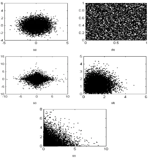
To test the performance of the proposed TASOM for the input distribution approximation, several experiments are developed in stationary and non-stationary environments. For this purpose, five different two-dimensional input distributions including Uniform distribution, Gaussian distribution, Exponential distribution, Laplacian distribution, and Rayleigh distribution are simulated. Each random vector of any of these distributions is composed of two independent and identically distributed one-dimensional random values. Specifically, we may say that the probability density function (pdf) of each distribution is f_X_,_Y(x,y)= f_X(x)f_X(y) for the

Uniform distribution, we have

   ≤ ≤ = otherwi 0 1 x 0 if 1 ) x ( f_X

for the Gaussian distribution,

2 2 / ) ( 2 ) ( 2 2 πσ σ m x X e x f − − =

where

−∞

<

x

<

∞

, σ >0, and m and σ are the mean and variance of random variable X,

respectively. The pdf of Exponential distribution is

x

X x e

f ₍ ₎₌_λ −λ _where_x_≥₀_and_λ_>₀_{. For}

Laplacian distribution we have | |

2 )

( x

X x e

f ₌α −α

where −∞<x<∞ and α >0. Finally, the pdf of

Rayleigh distribution is /2 2

2 ) ( α α x X e x x

f ₌ − _where

0

≥

x and α >0. In this paper, m=0 and 1

=

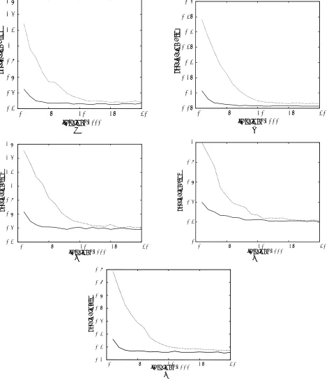
σ are set for the Gaussian distribution. For the Exponential distribution, we set λ=1. For the Laplacian and Rayleigh distribuitons, we set α=1. The five distributions with 10000 points are shown in Figures 1(a)-(e) for the Uniform, Gaussian, Exponential, Laplacian, and Rayleigh distributions, respectively. The test is carried out with 50 neurons forming one-dimensional lattices of neurons for both the basic SOM and TASOM networks. The expected approximated distortion of Equation 13 is used to compare the approximation error of the networks. The variations of the quantization error of the basic SOM and TASOM networks for the five distributions versus the number of iterations are depicted for every 1000 samples in Figures 2(a)-(e), where dashed lines represent the SOM’s behavior and solid lines represent the TASOM’s. It should be mentioned that different values for the basic SOM parameters were tested, and the results given here are for those giving the best quantization performance that could be achieved. In this paper, for the SOM network, the initial learning-rate and the initial width of neighborhood function parameters are η₀ =0.9 and σ₀ =N, respectively. Moreover, the time constants are

2000

2 1=τ =

τ . For the TASOM network, we use

1 . 0

=

=β

α α_s =β_s =0.01 15s_f =s_g =

N

j(0)=

σ η_j(0)=1.

The initial weight vector w_j(0), the scaling value )sl(0 , and the parameters Ek(0)and

) 0 ( 2k

E are small positive values which are randomly chosen.

(6)

adjustment of learning rates and neighborhood functions of neurons in the TASOM in which parameters are adjusted according to the environmental conditions. The second point is that the TASOM converges with less quantization error

than the basic SOM. This property is partly due to using separate learning rates and neighborhood functions for neurons. With separate learning rates and neighborhood functions, the TASOM network is able to locate neurons in the environment with

(a) (b)

(c) (d)

(e)

Figure 1. The five distributions used in the experiments each one represented by 10000 points. (a) the Gaussian distribution, (b) the

(7)

more flexibility than the basic SOM, which has only one learning rate and neighborhood function. Now consider the TASOM network of Figure

2(b) trained by the Uniform distribution. This network undergoes some change in its input space distribution. The first change is to Gaussian

0 5 10 15 20

0.2 0.4 0.6 0.8 1 1.2 1.4 1.6

iterations/1000

quatization error

0 5 10 15 20

0.05 0.1 0.15 0.2 0.25 0.3 0.35 0.4

qua

tiza

tion er

ro

r

iterations/1000

(a) (b)

0 5 10 15 20

0.2 0.4 0.6 0.8 1 1.2 1.4 1.6

iterations/1000

qu

at

iz

at

io

n er

ror

0 5 10 15 20

0 0.2 0.4 0.6 0.8 1

iterations/1000

q

u

a

tiz

a

tio

n e

rro

r

(c) (d)

0 5 10 15 20

0 .1 0 .2 0 .3 0 .4 0 .5 0 .6 0 .7 0 .8

itera tio ns/1000

quat

iz

at

io

n er

ro

r

(e)

Figure 2. The quantization error of TASOM and the basic SOM as iteration goes on where dotted lines represents the basic SOM and

(8)

distribution. Then it changes to Exponential, then Rayleigh, and finally Laplacian distributions. In fact, the TASOM network used in this experiment undergoes a very changing environment, which endure five complete changes in its input space while the TASOM is initialized only one time during its lifetime, irrespective of the changes in the environment. The quantization errors of the TASOM network in this case for the five distributions are shown in the third row of Table 1. For comparison, the quantization errors for the basic SOM and the TASOM networks are also presented and shown in the first and second rows of Table 1, respectively. The initial values of the parameters of the two networks are the same as those used in the previous experiments.

The TASOM is thus tested in two different cases. In one case, the initialization step of the TASOM algorithm is executed for each new environment. We call this case of using TASOM as “TASOM with initialization”. This case is surely stationary, since we have to initialize the weight vectors and other parameters of the TASOM network for learning its environment, and it is assumed that the statistical characteristics of the environment do not change with time. The basic SOM can be used only in this case.

The other case of using the TASOM network is a non-stationary case in which it is assumed the environment may be faced with some changes in its statistical characteristics as time goes on. In this case, the initialization step is used only the first time that the TASOM network is trained. When the distribution of the environment changes, the network has to learn the new environment with the values of the weights and parameters that have been learned with its former environment. The ability of TASOM in learning the new environment is solely dependent on the learning rate and neighborhood width updating proposed in

the TASOM algorithm. We call this case “TASOM without initialization”.

According to Table 1, most of the time, the errors for the TASOM without initialization is slightly lower than the case where the TASOM with initialization is used. The basic SOM produces higher errors than the TASOM with initialization and TASOM without initialization. In other words, the TASOM network performs well in non-stationary as well as stationary environments. The TASOM network uses separate learning rate and neighborhood width for each neuron of the network. So, the neurons of TASOM are more flexible than the basic SOM to represent the input vectors. This way, the TASOM networks obtain better performance than the basic SOM as shown in Table 1.

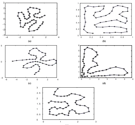
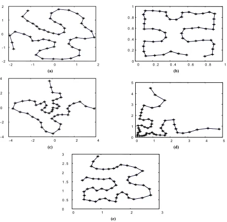
To assure that the TASOM has preserved topological ordering in the mentioned experiments, the converged weights of TASOM for the five distributions with initialization for each distribution, the weights of the SOM for the five distributions, and the converged weights of the TASOM for the four distributions without initialization are all presented in Figures 3(a)-(e), 4(a)-(e), and 5(a)-(d), respectively. According to these Figures, the TASOM always preserves topological ordering.

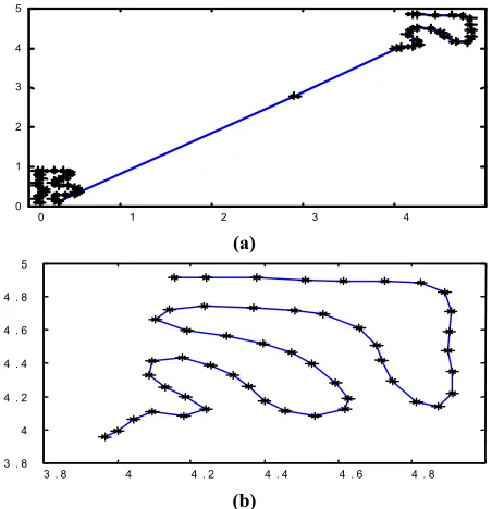
It may be interesting to see the stages during which the input distribution changes while the TASOM moves its weights to gradually represent the most recent distribution. Assume that the TASOM network converged to represent the two-dimensional Uniform distribution in the region [0,1]×[0,1] faces a new Uniform input distribution in the region

] 5 , 4 [ ] 5 , 4

[ × . Figure 3(b) shows the TASOM weights for the former Uniform distribution. Figure 6(a) demonstrates the intermediary stage of convergence of the TASOM weights toward the new Uniform TABLE1. The Quantization Error of the Basic SOM, the TASOM with Initialization, and the TASOM Without Initialization

for the Five Input Distributions.

SOM \ Distribution Unifor m

Gaussian Exponential Laplacian Rayleigh

Basic SOM 0.0651 0.2866 0.2283 0.4108 0.1788

TASOM with initialization 0.0592 0.2714 0.2182 0.4053 0.1662

TASOM without initialization

(9)

distribution. At the end, Figure 6(b) shows the converged weights for the new Uniform distribution, which not only preserves topological ordering, but also distributes uniformly in the new input space and completely covers it.

It seems that The TASOM moves its weights in topological order, no matter what happens in the environment. Moreover, it adapts its weights to the new environment in an elegant fashion. This means that the weights gradually leave the old distribution and move gradually toward the clusters of the new distribution. This phenomenon reminds us of the memory of our brains. The past memory

remains refresh as long as new sensory data emphasize that. If new sensory inputs different from those of the past ones are received, our memory tries to represent and memorize the recent data. However, forgetting the past memory and memorizing the new one is also gradual in our brain, we don’t forget past memory and we also don’t memorize the new one suddenly.

CONCLUDING REMARKS

The decreasing time-dependent learning

-4 -2 0 2 4

-3 -2 -1 0 1 2 3

0 0 .2 0 . 4 0 . 6 0 .8 1 0

0 . 2 0 . 4 0 . 6 0 . 8 1

(a) (b)

- 6 - 4 - 2 0 2 4

- 5 0 5

0 1 2 3 4 5 6

(c) (d)

0 1 2 3

0 0 . 5 1 1 . 5 2 2 . 5 3

(e)

(10)

parameters of the SOM lower the incremental learning capability of the algorithm in response to varied environments. In this paper, a modified SOM algorithm called “TASOM” with neighborhood function was proposed to automatically adjust the learning rate parameter and the neighborhood function of each output neuron. Each output neuron is assumed to have its own learning rate and neighborhood function, which are updated repeatedly in the proposed SOM algorithm in response to new input samples.

The proposed TASOM was tested in stationary

environments, and was compared to the basic SOM for input approximation. According to these tests, the TASOM can be claimed to converge with fewer iterations than the basic SOM. Moreover, the quantization errors of the TASOM are lower than the errors of the basic SOM. The TASOM was also tested in non-stationary environments in which the input distribution completely changes to another distribution. There is no need to reinitialize the TASOM in response to changes in the input distribution. Experimental results confirm this claim. In the TASOM, learning of the new

- 2 - 1 0 1 2

0 0 . 2 0 . 4 0 . 6 0 . 8 1

(a) (b)

- 4 - 2 0 2 4

0 1 2 3 4 5

(c) (d)

0 1 2 3

0 0 . 5 1 1 . 5 2 2 . 5 3

(e)

(11)

distribution is gradual, similar to the human memory, which constantly and gradually updates itself to the more recent data while forgets the old memory in the long run.

These experiments suggest that the TASOM is suitable for both stationary and non-stationary environments. In fact, the TASOM learns continuously from its environment, and only a one- time initialization is needed for it to work in its possibly changing environment.

REFERENCES

1. Kohonen, T., “Self-Organized Formation of Topologically Correct Feature Maps”, Biological Cybernetics, Vol. 43, (1982), 59-69.

2. Chiuch, T. D., Tang, T. T. and Chen, L. G., “Vector Quantization Using Tree-Structured Self-Organizing Feature Maps”, In Applications of Neural Networks to Telecommunications (J. Alspector, R. Goodman, and T. X. Brown, eds.), Hillsdale, NJ: Lawrence Erlbaum, (1993), 259-265. 3. Oja, E., “Self-Organizing Maps and Computer Vision”, In

Neural Networks for Perception (H.Wechsler, ed.), San Diego, CA: Academic Press, Vol. 1, (1992), 368-385.

- 2 - 1 0 1 2 3

- 2 - 1 . 5 - 1 - 0 . 5 0 0 . 5 1 1 . 5 2

0 1 2 3 4 5

(a) (b)

- 6 - 4 - 2 0 2 4

- 5 0 5

0 1 2 3 4

0 0 . 5

1 1 . 5

2 2 . 5

3

(c) (d)

Figure 5. (a) The TASOM network of Figure 2(b) trained by the Uniform distribution faces the Gaussian distribution. (b) The

TASOM network of Figure 5(a) faces the Exponential distribution. (c) The TASOM network of Figure 5(b) faces the Laplacian distribution. (d) The TASOM network of Figure 5(c) faces the Rayleigh distribution.

0 1 2 3 4

0 1 2 3 4 5

(a)

3 . 8 4 4 . 2 4 . 4 4 . 6 4 . 8 3 . 8

4 4 . 2 4 . 4 4 . 6 4 . 8 5

(b)

Figure 6. (a) The topographic map of the TASOM in an

(12)

4. Ritter, H. J., Martinez, T. M. and Schulten, K. J., “Neural Computation and Self-Organizing Maps: An Introduction, Reading MA”, Addison Wesley, (1992).

5. Kohonen, T., “The Neural Phonetic Typewriter,” Computer, Vol. 21, (1988), 11-22.

6. Amerijckx, C., Verleysen, M., Thissen, P. and Legat, J., “Image Compression by Self-Organized Kohonen Map”,

IEEE Trans. on Neural Networks, Vol. 9, No. 3, (1998), 503-507.

7. Haykin, S., “Neural Networks”, Prentice Hall, New Jersey, (1999).

8. Heskes, T. and Kappen, B., “Neural Networks Learning in a Changing Environment”, IJCNN, (1991), 823-828. 9. Haese, K., “Organizing Feature Maps With

Self-Adjusting Learning Parameters”, IEEE Trans. On Neural Networks, Vol. 9, No. 6, (1998), 1270-1278.

10. Maillard, E and Gresser, J., “Reduced Risk of Kohonen’s Feature Map Non-Convergence by an Individual Size of the Neighborhood”, IEEE International Conference on Neural Networks, Vol.2, (1994), 704-707.

11. Kim, C. W., Cho, S. and Lee, C. W., “Fast Competitive Learning With Classified Learning Rates for Vector Quantization”, Signal Processing Image Communication, Vol. 6, No. 6, (1995), 499-505.

12. Shah-Hosseini, H. and Safabakhsh, R., “Automatic Adjustment of Learning Rates of the Self-Organizing Feature Map”, Accepted for Publication in Scientia Iranica.

13. Shah-Hosseini, H. and Safabakhsh, R., “A Learning Rule Modification in the Self-Organizing Feature Map Algorithm,”

Fourth Int. CSI Computer Conference, Tehran, Iran, (1999), 1-9.

14. Shah-Hosseini, H. and Safabakhsh, R., “TASOM: The Time Adaptive Self-Organizing Map”, Proc. Int’l Conf. Information Technology Coding and Computing, IEEE Press, Las Vegas, Nevada, (2000), 422-427.

15. Shah-Hosseini, H. and Safabakhsh, R., “Pattern Classification by the Time Adaptive Self-Organizing Map”, Proc. IEEE Int’l Conf. Electronics, Circuits and Systems, Beirut, Lebanon, (December 17-20, 2000), 495-498.

16. Kangas, J. A., Kohonen, T. and Laaksonen, J. T., “Variants of Self-Organizing Maps”, IEEE Trans. on Neural Networks, Vol. 1, No. 1, (1990), 93-99.

17 Trautmann, T. and Denoeux, T., “Comparison of Dynamic Feature Map Models for Environmental Monitoring”, IEEE Int. Conf. On Neural Networks, Vol.1, (1995), 73-78.

18. Datta, A. Pal, T. and Parui, S. K., “A Modified Self-Organizing Neural Net for Shape Extraction,” Neurocomputing, Vol. 14, No. 1, (1997), 3-14.

19. Chau-Yun, H. and Hwai-En, W., “An Improved Algorithm for Kohonen’s Self-Organizing Feature Maps”, IEEE Int. Conf. On Circuits and Systems, Vol. 1, 328-331.

20. Blackmore, J. and Miikulainen, R., “Incremental Grid Growing: Encoding High Dimensional Structures to a Two-Dimensional Feature Map”, IEEE International Conference on Neural Networks, Vol. 1, (1993), 450-455. 21. Fritzke, B., “Growing Cell Structures-a Self-Organizing

Network for Unsupervised and Supervised Learning”,

Neural Networks, Vol. 7, (1994), 1441-1460.