The Impact of Seasonal Unit Roots and Vector ARMA Modeling on Forecasting Monthly Tourism Flows

Full text

(1)The impact of seasonal unit roots and vector ARMA modelling on forecasting monthly tourism °ows¤ Patrik Gustavssona and Jonas NordstrÄomb a Trade Union Institute for Economic Research and Stockholm School of Economics, Sweden b. Department of Economics, Umeº a University, Sweden. Abstract The e®ect of imposing di®erent numbers of unit roots on forecasting accuracy is examined using univariate ARMA models. To see whether additional information improves forecasting accuracy and increases the informative forecast horizon, we crossrelate the time series for inbound tourism in Sweden for di®erent visitor categories and estimate vector ARMA models. The mean-squared forecast error for di®erent ¯lters indicates that models in which unit roots are imposed at all frequencies have the smallest forecast errors. The results from the vector ARMA models with all roots imposed indicate that the informative forecast horizon is greater than for the univariate models. Out-of-sample evaluations indicate, however, that the univariate modelling approach may be preferable. Keywords: Seasonality, tourism, demand analysis, VARMA, forecasting. JEL classi¯cation: C22, C32, C53, D12. ¤. Ä We thank Kurt BrÄannÄas, JÄorgen HellstrÄ om, Xavier de Luna, and Lars-Erik Oller for helpful. comments. Financial support from the Swedish Council for Research in the Humanities and Social Sciences and the Jacob Wallenberg Research Foundation to the ¯rst author and from the Swedish Transport and Communications Research Board to the second author is gratefully acknowledged..

(2) 2. 1. Introduction. The perishable nature of tourism products and the many capacity-related decisions that have to be made well in advance make accurate forecasting of the demand for tourism particularly important. This implies that even small improvements in forecasting the demand for tourism are very valuable. In a survey of tourism demand forecasting, Witt and Witt (1995) pointed out that econometric forecasts did not rank very high in terms of accuracy. In addition, Garcia-Ferrer and Queralt (1997) found the contributions of price and income proxy variables to be negligible in terms of goodness of ¯t and forecasting, when compared to alternative univariate models. NordstrÄom (1999) found that prices and, in particular, changed preferences have an important in°uence on inbound tourism in Sweden; however, from a forecasting point of view, pure time-series models turn out to be as good as the economic models. One reason for the relatively modest short- and medium-term forecasting performance of the economic models was the di±culty in obtaining good forecasts of the price variables. Since a large part of the variation in inbound tourism can be explained by taste changes (NordstrÄom 1999), the largest gain in forecasting accuracy is probably not merely the result of better prediction of the price variables. Instead, better predictions of tourism demand may be expected by estimating and forecasting tourism series jointly with other tourism series, in which information on taste and price changes are already incorporated. These predictions are also gained at a lower cost. Since the form of such models is determined by the data alone, the analysis demands a °exible structure. As structural changes or regime shifts are important aspects of the real world, di®erent transformations of the series should be made in order to make forecasts robust. Clements and Hendry (1996) showed that forecasts from a vector autoregression in di®erences (DVARs) may be more robust than models in levels with respect to certain forms of structural change. However, as pointed out by LÄ utkephol (1991, pp. 232-233), a linearly transformed ¯nite order VAR(p) process will, in general, not admit a ¯nite order VAR representation. We therefore use vector autoregressive moving average (VARMA) models to investigate whether information from di®erent tourism series improves the forecasting performance of.

(3) 3 tourism demand models. In this study, we focus on monthly tourism °ow data that are characterised by pronounced seasonal patterns. As the identi¯cation process for VARMA models can be cumbersome for high-frequency data, as a consequence of the long lag polynomials, we begin the analysis with the univariate counterpart. The Box and Jenkins (1970) modelling framework rests on applying the seasonal di®erence 1 ¡ B 12 , where. B is the back-shift operator B k yt = yt¡k , in the stationarity-producing phase of the procedure. Factorising the 1 ¡ B 12 polynomial as. p p 1¡B 12 = (1¡B)(1+B)(1+B 2 )(1+B+B 2 )(1¡B+B 2)(1+ 3B+B 2 )(1¡ 3B+B 2 ). shows that the seasonal di®erence operator implicitly imposes a root on the zero frequency, as well as on all seasonal frequencies ¼, ¼=2, 2¼=3, ¼=3, 5¼=6, and ¼=6 corresponding to the periods 2, 4, 3, 6, 12=5, and 12. For most empirical series, one would expect to ¯nd a unit root at the zero frequency and possibly at some of the seasonal frequencies (e.g., Clements and Hendry 1997, Franses 1996, Hylleberg 1992, Beaulieu and Miron 1993). Thus, there is a risk of over-di®erencing with the 1 ¡ B 12 ¯lter.. We therefore start the univariate analysis with an investigation of the e®ects. of imposing di®erent sets of seasonal unit roots on the model. As pointed out by Clements and Hendry (1997), there is little evidence in the literature on the e®ect of imposing seasonal unit roots on forecast accuracy. Exceptions are some studies on quarterly data. For example, Clements and Hendry (1997) compared the forecast performance of a sequence of rolling forecasts of autoregressive models, and Paap, Franses and Hoek (1997) compared the forecast performance of autoregressive seasonal unit root models and seasonal mean-shift models. Results in Clements and Hendry (1997) indicated that imposing roots at all frequencies led to at least as good forecasting performance as did imposing the smaller number of roots suggested by the HEGY (Hylleberg, Engle, Granger and Yoo 1990) procedure. Paap et al. (1997) found, on the other hand, that the empirical seasonal mean-shift models produced more accurate forecasts than did models that incorrectly imposed too many seasonal unit roots. The simulation study in Paap et al. (1997) indicated, however, that the number of changing seasons may have some e®ect on the results. If one or more.

(4) 4 seasonal unit roots were present in the Monte Carlo experiment, the model selected by the HEGY procedure out-performed the seasonal mean-shift model. This paper is organised as follows. In Section 2 we present the data on the monthly number of guest nights and utilise a state-space model to describe the components in the time series. In Section 3.1, we perform a statistical test of unit roots, and investigate whether the series become stationary after imposing the unit roots indicated by the test or by some other ¯lter. The forecasting performance of the univariate ARMA models with di®erent unit roots imposed is evaluated in Section 3.2. The potential improvements in forecasting performance by cross relating the series is studied in Section 4. Section 5 concludes.. 2. Data. In this study we analyse the monthly numbers of guest nights spent in Swedish hotels and cottages for the ¯ve largest national categories visiting Sweden. This type of data is likely to be integrated on the zero and some seasonal frequencies, due to important long-run and seasonal components. The economics underpinning this pattern may depend on a large number of factors, such as increased leisure time, the activities undertaken by the visitors, weather conditions, the distance visitors have to travel, changing transport costs, or changing preferences. Although the underlying reason for the changing seasonal pattern is an interesting issue, it is beyond the scope of this paper. Accommodation statistics of this kind have been collected by Statistics Sweden since January 1978, and we use this data through December 1996. In 1994, the ¯ve largest national categories were, in decreasing order, German, Norwegian, Finnish, US, and Danish visitors. A time series plot of the number of guest nights in hotels and cottages is shown in Figure 1. The ¯gure reveals a strong seasonal pattern in all series, with the cottage series more irregular than the hotel series. Another way of obtaining a descriptive analysis of the trend and amount of seasonal variation in the series, is to put the series in state-space form (see e.g. Harvey 1989). Here, we estimated the guest-night series on a stochastic trend and.

(5) 5. Norway hotel. 12.50. 11.50. 11.63. 9.75. 10.75. 8.00. 9.88. 6.25. 9.00. Norway cottage. 4.50. Finland hotel. 11.50 10.75 10.00 9.25 8.50. Denmark hotel. 11.00. 10.00 8.25 6.50 4.75 3.00 12.00. 10.38. 10.50. 9.75. 9.00. 9.13. 7.50. 8.50. Finland cottage. Denmark cottage. 6.00. Germany hotel. 12.50 11.38 10.25 9.13 8.00. 11.50. Germany cottage. 9.38 7.25 5.13 3.00. US total. 12. 78 80 82 84 86 88 90 92 94 96. Year. 11 10 9 8. 78 80 82 84 86 88 90 92 94 96. Year. Figure 1: Natural logarithms of inbound guest nights in hotels and cottages in Sweden, 1978-96..

(6) 6. 11.00. (a) Norway hotel trend component. 2. 10.67. 1. 10.33. 0. 10.00. -1 78 80 82 84 86 88 90 92 94 96. 0.00. 78 80 82 84 86 88 90 92 94 96. (c) Month 1 to 3. 0.60. -0.25. 3. 0.30. -0.50. 2. 0.00. 1. -0.75 -1.00. (d) Month 4 to 6 6 5. 4. -0.30 -0.60. 78 80 82 84 86 88 90 92 94 96 2. (b) Norway hotel seasonal component. (e) Month 7 to 9. 78 80 82 84 86 88 90 92 94 96 0.20. (f) Month 10 to 12. 7 1. 8. 0. 9. -1. 10 -0.13 11 -0.47. 12. -0.80 78 80 82 84 86 88 90 92 94 96. 78 80 82 84 86 88 90 92 94 96. Year. Year. Figure 2: Trend and seasonal component of logarithms of Norwegian guest nights in hotels, (1978-96)..

(7) 7. 9.50. (a) Norway cottage trend component. 3.50. 8.75. 2.00. 8.00. 0.50. 7.25. -1.00. 6.50. -2.50 78 80 82 84 86 88 90 92 94 96. 1. (b) Norway cottage seasonal component. 78 80 82 84 86 88 90 92 94 96. (c) Month 1 to 3. 2. (d) Month 4 to 6. 3 0. 1. 4. 2 6 -1. 0 5. 1 -2. -1 78 80 82 84 86 88 90 92 94 96. 3. (e) Month 7 to 9. 78 80 82 84 86 88 90 92 94 96 1. (f) Month 10 to 12. 7 2. 0. 11. 8 1 9. 0 -1. -1. 10. -2. 12. -3 78 80 82 84 86 88 90 92 94 96. Time. 78 80 82 84 86 88 90 92 94 96. Time. Figure 3: Trend and seasonal component for logarithms of Norwegian guestnights in cottages, (1978-96)..

(8) 8 a stochastic trigonometric seasonal component. The estimated components of the Norwegian series are revealed in Figures 2 and 3. Figures 2a and 3a indicate that the series may not be trend stationary. Therefore we expect to ¯nd a unit root at the zero frequency. The seasonal component is plotted in Figures 2b and 3b. As revealed in Figure 2b, the seasonal component for the Norwegian hotel series is rather stable. The seasonal component for the Norwegian cottage series in Figure 3b; however, shows a changing pattern. Figure 3b also indicates that the amplitude of the seasonal component for the summer months decreases over the sample period. In Figures 2c-2f and 3c3f we have plotted the seasonal contribution from each month. If the seasonal component is deterministic around seasonal intercept dummy variables, then the lines in Figures 2c-2f and 3c-3f would be horizontal straight lines. As expected, the graphs in Figure 2c-2f only reveal minor changes, hence we do not expect to ¯nd seasonal unit roots on all seasonal frequencies in the Norwegian hotel series. From the monthly contributions in Figures 3c-3f; we can see that the Norwegian cottage series is probably not deterministic around seasonal intercept dummy variables. The ¯gure reveals increases for the months February to April, while the traditional holiday months, i.e. June, July, and August, indicate decreases. Altogether this indicates a non-constant seasonal pattern. However, at this stage we can not rule out the possibility that the seasonal component in the Norwegian cottage series is deterministic around seasonal intercept dummy variables and deterministic seasonal trends.. 3. Testing for seasonal unit roots. To formally test for unit roots at the zero and seasonal frequencies, we use the test presented by Beaulieu and Miron (1993) [BM] and Taylor (1998). The test presented by Taylor is an extension of BM's test to allow for seasonal drifts under the null hypothesis. Taylor's and BM's procedure is analogous to the approach developed by Hylleberg, Engle, Granger, and Yoo (1990) and is based on the following regression.

(9) 9 equation: Á(B) M12 yt =. 12 X k=1. °k yk;t¡1 +. 12 X. ¯m Dm;t +. m=1. 12 X. ±m Dm;t t + "t;. t = 1; 2; :::; T: (1). m=1. In regression (1), the yk;t , k = 1; :::; 12, constitute a set of linear ¯lters of yt , whose exact form is given in BM (p. 308), Dm;t is the seasonal intercept dummy for month m, m = 1; :::; 12, and Á(B) = (1 ¡ Á1B ¡ ::: ¡ Áp B p) is a lag polynomial of order p. In the BM test, the third expression on the right-hand side is replaced by ±t, i.e. with a common trend for all seasons. The applied ¯lters separate out unit roots corresponding to frequencies 0, ¼, ¼=2, 2¼=3, ¼=3, 5¼=6 and ¼=6, such that the restriction °1 = 0 in (1) implies a zero-frequency unit root, while °2 = 0 implies a ¼ or Nyquist frequency unit root, and ¼k = ¼k+1 = 0 implies a unit root at the corresponding frequency pair (k, k + 1), k = 3, 5, 7, 9, 11. The goal is to test hypotheses about a particular unit root without taking a stance on whether other seasonal or zero frequency unit roots are present. In order to test hypotheses about various unit roots, the OLS test statistics based on (1) are compared to the critical values tabulated in BM (1993) and Taylor (1998). For frequencies 0 and ¼, we examine the relevant t-statistic for °k = 0; k = 1; 2 against the alternative that °k < 0. For the other frequencies, we test °k = °k+1 = 0, k = 3; 5; 7; 9; 11; with an F -statistic. Additional lags of the dependent variable are included to capture autocorrelation in the errors. The order p is based on LM-tests of ¯rst to 36th order of serial correlation in the residuals. We consider di®erent speci¯cations of the deterministics and allow for the possibility of seasonal intercepts together with a time-trend variable or seasonal timetrend variables. This last case permits the drift in a seasonal random walk data generating process (DGP) to di®er across seasons, thereby allowing the amplitude of the variations across the seasons of the deterministic component in the level of the time series to vary (linearly) over time. One further implication of the seasonal trends formulation in (1) is that it allows one to test the unit root null hypothesis against the alternative of trend stationarity not only at the zero frequency, but also at the seasonal frequencies (Smith and Taylor, 1999). The latter tests are not possible with the formulation of BM..

(10) 10. 3.1. Test results. Initially all series were tested with Taylor's (1998) approach using both seasonal dummies and trends. An F -test could not reject the null of separate seasonal trends at a 10 percent signi¯cance level for any of the series. However, Figure 3 indicates that seasonal trends may be appropriate for the Norwegian cottage series. In the following, we base our analysis on BM's test as we do not wish to include unnecessary deterministic seasonal components in the test (see Taylor, 1997). As the F -test ruled out the seasonal trends speci¯cation, we assume that the BM test has the same alternative hypothesis as Taylor's test. Since there is no clear-cut evidence whether the Norwegian cottage series have deterministic seasonal trends or not, we tabulate results from both BM's and Taylor's speci¯cation for this series. In Table 1, the outcome of seasonal unit root tests using the BM (1993) speci¯cation is presented. The results are based on data up to 1994:12. Results indicate that the non-seasonal unit root appears to be present in all time series. In addition, the BM tests reveal that most of the series have one or two seasonal unit roots, indicating a changing seasonal pattern caused by seasonal stochastic trends. For the hotel series and US total series, results are the same as when seasonal trends are included, an exception is the Danish hotel series were unit roots at the ¼=2 and 2¼=3 frequencies where indicated in addition to the roots revealed in Table 1. However, for all cottage series there is a di®erence in the number of identi¯ed unit roots, depending on whether a common trend or seasonal trends are included in the test. At a 5 percent signi¯cance level, the unit root test with seasonal trends indicated a unit root at the zero frequency and trend-stationary seasons. For the US series and German cottage series, Table 1 indicates a deterministic seasonal pattern around seasonal intercept dummies. This is possibly due to longer travel time or distance for these trips, which suggests that they are undertaken during a longer vacation period. For none of the logarithmically transformed time series does the BM test in Table 1 indicate use of the 1 ¡ B 12 di®erencing ¯lter.. The robustness of the test result has been checked by restimating (1) over the. full sample. Generally, the same unit roots were found. Exceptions were the Norwegian and Danish hotel series, for which additional seasonal unit roots were found..

(11) 11. Table 1: Results of tests for seasonal unit roots. 0. ¼. ¼=2. 2¼=3. ¼=3. 5¼=6. ¼=6. Lag. °1. °2. F3;4. F5;6. F7;8. F9;10. F11;12. Norway hotel Finland hotel Denmark hotel Germany hotel Norway cottage Finland cottage Denmark cottage Germany cottage US total. 3 1 2 -. 1.95 0.75 -1.25 -0.11 1.26 -0.21 -0.80 -2.05 3.06. -3.39 -3.62 -3.69 -3.93 -3.74 -3.86 -5.31 -3.84 -4.74. 13.23 8.75 8.00 8.48 7.64 9.63 5.95 8.00 20.52. 18.94 9.95 10.87 15.57 10.36 16.24 10.10 13.81 20.91. 9.41 15.46 7.39 3.84 8.14 15.51 3.46 6.24 19.56. 11.23 6.94 4.87 9.42 10.94 4.42 10.00 11.61 21.16. 3.39 4.53 13.28 7.78 2.64 8.17 2.51 7.23 12.94. Norway cottage*. 1, 12, 24. 0.27. -3.90. 10.77. 15.78. 15.53. 15.75. 9.75. Series. Notes:*Seasonal dummies and seasonal trends have been included in the unit root test, otherwise seasonal dummies and a common trend have been included in the unit root test. The critical values at the percent level of the common trend and seasonal dummies are °1 = -3.28, °2 = -2.75, and F = 6.23. The critical values at the 1 percent level of the common trend and seasonal dummies are °2 = -3.31, and F = 8.33. * The critical values at the 5 percent level of the seasonal trends and dummies are °1 = -3.32, °2 = -3.31 and F = 9.13. * The critical values at a 1 percent level of the seasonal trends and dummies are °2 = -3.86 and F = 11.56. Lag indicates which lag of Á(B)y13t is included.. As pointed out by Perron (1990) and Franses and Vogelsang (1998), an increased number of unit roots can be a result of neglected deterministic mean shifts, and at a 5 percent signi¯cance level we identi¯ed a mean shift for both series in 1994. The test for the Norwegian hotel series may also su®er from low power, since we have to increase the order of the lag polynomial to 5 (lags 1,3,4, and 5) (Hylleberg 1995). To see whether the series become stationary after imposing the identi¯ed roots in Table 1, the ¯ltered series are again tested for unit roots. That is, for the Norwegian and Finnish hotel series we impose roots on the zero and ¼=6 frequencies with the p ¯lter (1 ¡ B)(1 ¡ 3B + B 2 ), for the Danish hotel series on the zero and 5¼=6 p frequencies with the ¯lter (1 ¡ B)(1 + 3B + B 2), and so on for the other series. Results indicate that only in one case (Norwegian holiday villages) do these ¯lters. lead to a stationary series. Generally, on the ¯ltered series we found unit roots at both the zero frequency and some of the seasonal frequencies. However, after.

(12) 12 reducing the identi¯ed ¯lter to 1 ¡. p. 3B + B 2 for the Norwegian and Finnish hotel. series we obtained stationarity. The same ¯lter also turned out to generate stationary processes for all series in Table 1 that have one or more seasonal unit roots. On the other hand, imposing roots at all frequencies, as implicitly recommended by the Box-Jenkins approach, tests indicated that a unit root was generally identi¯ed at the zero frequency. Only the German and Finnish holiday villages series become stationary using the 1 ¡ B 12 di®erence.1. 3.2. Forecasting performance. In this section we estimate univariate ARMA(p; q) models to compare the forecast accuracy between models where the smallest number of unit roots has been imposed to obtain a stationary series, to that of a series where unit roots have been imposed at all frequencies. The ARMA models to be estimated are written as Ã 12 ! X À(B)yt = À(B) 'm Dm;t + Á¡1 (B)µ(B)ut ; m=1. for the models based on the 1 ¡ B di®erence and the BM test, whereas the models. corresponding to the DGP of Taylor's test are written as Ã 12 ! 12 X X À(B)yt = À(B) 'm Dm;t + ¸m Dm;t t + Á¡1(B)µ(B)ut ; m=1. m=1. where À(B) is the ¯lter applied to the series, Á(B) = 1 ¡ Á1 B ¡ ::: ¡ ÁpB p and µ(B) = 1 + µ1 B + ::: + µq B q . To obtain a stationary process the annual frequency p ¯lter, 1 ¡ 3B + B 2 , has been applied to all series, except the German cottage and. US total series to which a ¯rst di®erence has been applied. The German cottage series became stationary once a ¯rst di®erence was imposed, and for the US total series the ¯rst di®erence turned out to be the best alternative to a twelth-di®erence,. although the BM test indicated a root on the ¼=6 frequency.2 To identify the models we started with a general ARMA(p; q) model, with an initial lag structure 1. However an F -test over all frequencies indicate stationarity using a 12th di®erence (at a 5. percent signi¯cance level). 2. The BM test indicates that other seasonal ¯lters yield unit roots at several seasonal frequencies..

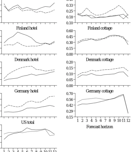
(13) 13 (p; q) of three years. This tentative speci¯cation was thereafter gradually reduced by minimising the Schwartz Bayesian information criterion (BIC). The ARMA models are estimated by non-linear least squares using EViews 2.0. The estimation results, which are available from the authors upon request, suggest that the 1 ¡ B 12 transformed series generally have roots close to one in the MA polynomial, which is to be expected since the BM tests indicate that the series. are over-di®erenced. On the other hand, the models with the smaller number of imposed unit roots have roots close to one in the AR polynomial. The results also indicate that the models for the 1¡B 12 transformed series have a more parsimonious parameter representation than models based on other ¯lters. The forecasts are obtained as follows. The identi¯ed models are estimated on data up to 1994:12. Then, 1994:12 is taken as the forecast origin for forecasting 1 up to 12 steps ahead. The model is then re-estimated on data up through 1995:1, with the form of the model unchanged. 1995:1 is then taken as the forecast origin, and so on, subject to the constraint that we have data on the period being forecasted (the sample ends in 1996:12). This gives 24 one-step forecasts, 23 two-step forecasts, and so on. The forecasts are then transformed from the di®erentiated form to forecasts in log levels. By comparing the forecasts in levels we do not need to calculate the generalised forecast error second moment (GFESM) measure developed by Clements and Hendry (1993). The means, variances, and mean square errors are then calculated on the forecast error for each forecast horizon. In Figure 4 we have plotted the mean squared forecast errors (MSFE) for each forecast horizon. As the ¯gure reveals it is more di±cult to obtain good forecasts for the cottage series compared to the hotel series. Although the di®erence in forecast performance between the di®erent ¯lters is small, the 1 ¡ B 12 ¯lter (solid line). generally produces the smallest MSFE. The ¯gure also indicates that the Norwegian cottage model based on a 1 ¡B 12 di®erence or a 1 ¡B di®erence and seasonal trends. produces equally good forecasts. The calculated variance of the forecast errors shows the same pattern as the MSFE but is smaller for the 1 ¡ B 12 di®erentiated series. in all cases except for the Finnish hotel series. The mean of the forecast errors, however, indicates that the ¯lter with the smaller number of imposed unit roots.

(14) 14. 1.00. Norway hotel. 0.40. 0.75. 0.33. 0.50. 0.25. 0.25. 0.18. 0.00 0.40. 0.10. Finland hotel. 0.60. 0.30. 0.45. 0.20. 0.30. 0.10. 0.15. 0.00 0.80. Finland cottage. 0.00. Denmark hotel. 0.20. 0.60. 0.15. 0.40. 0.10. 0.20. 0.05. 0.00 0.40. Norway cottage. Denmark cottage. 0.00. Germany hotel. 0.70. 0.30. 0.56. 0.20. 0.42. 0.10. 0.29. 0.00. Germany cottage. 0.15. US total. 0.30. 1 2 3 4 5 6 7 8 9 10 11 12. Forecast horizon. 0.22 0.15 0.07 0.00 1 2 3 4 5 6 7 8 9 10 11 12. Forecast horizon. Figure 4: Mean square forecast error for the logarithmic series in levels. Solid line p (1 ¡ B 12)-di®erentiated series; broken line (1 ¡ 3B + B 2 )-di®erentiated series;. dotted line (1 ¡ B)-di®erentiated series; broken line with dots (1 ¡ B)-di®erentiated series with seasonal trends. The MSFE for the Norwegian hotel series have been. multiplied by 100; the MSFE for the other hotel series and the US total series have been multiplied by 10..

(15) 15 yields better forecasts in six out of nine cases. However, the calculated mean of the forecast errors indicate a tendency to underestimate the actual number of guest nights, especially for the 1 ¡ B 12 di®erentiated. series. Whether the under-estimation is a result of an increasing positive trend in the underlying series or a result of a bias in the parameter estimates is di±cult to say. According to Granger (1996), there is a tendency to under-estimate change. We have therefore performed a small Monte Carlo study for the (1¡ÁB)yt = (1¡µB 12 )ut process to study the small sample properties of the estimator.3 The results indicate that there is a bias towards zero for the AR parameter, which increases as the absolute value of the autoregressive parameters increases. The bias also increases as the absolute value of the moving average parameters increases, but to a smaller extent. However, the bias was never found to be larger than two standard deviations. In the positive autoregressive parameter space with µ = ¡0:6 and n = 240, the 6-steps. ahead forecast error has a mean ranging from -0.06 to -0.02. For the same parameter settings, the empirical mean squared forecast error (EMSFE) for 6 steps ahead is 3% larger than the theoretical MSFE, ¾u2 (1 ¡ Á2£6 )=(1 ¡ Á2), when 0 < Á. 6-10% larger for 0:7. Á. 0:6,. 0:9, and 15% larger for the unit root case, Á = 1. Thus,. to some extent the under-estimation of the number of guest nights is a result of a downward bias in the autoregressive parameters.. 4. Can the quality of the forecast be improved?. Since the results in the previous section indicated that the 1 ¡ B 12 di®erence was. preferable, compared to other seasonal ¯lters, we here study the e®ects of adding information from other tourism series to the `Box-Jenkins' ARMA model. As tourism series for di®erent countries tend to correlate, and these series contain information from prices, income and other sources, the forecast performance may be improved by joint modelling. To see whether the forecast accuracy can be improved for the Finnish hotel series 3. We employed four sample sizes n = f60, 120, 240, 480g and conducted 1000 replications in the. parameter space [-1,1] with an interval of 0.1..

(16) 16. Table 2: Estimated parameters of the echelon VARMA representation. A1. Series. 2. Norway 0:60 hotel 6 (0:06) 6. 6. Finland 4 hotel. 0. A3 32. 32 0:19 0:03 7 6 (0:07) (0:05) 7 6 76 76 76 76 0:34 5 4 0:10 0:15 5 4 (0:06) (0:07) (0:07) 0. p6 = 0.73, p12 = 0.57, p18 = 0.28.. A1 2. 3 7. Norway 4 0:04 0:20 5 cottage (0:04) (0:08). 2. 3 0:32 0 6 (0:10) 7 6 7 6 7 4 0 0 5. p6 = 0.86, p12 = 0.85, p18 = 0.80.. M12. 32 0:15 ¡0:05 6 (0:06) (0:05) 7 76 76 0:15 0:14 5 4 (0:08) (0:06). A12. Norway 0:48 ¡0:09 hotel 6 (0:08) (0:12) 7 6 7. 6. A8. A24 2. 0. 3 ¡0:52 ¡0:02 (0:07) (0:06) 7 7 7 0:11 ¡0:57 5 (0:09) (0:07) M12. 0. 6 6 6 4 0:23 0 (0:03). 3 7 7 7 5. 2. 3 0:11 ¡0:23 6 (0:14) (0:16) 7 6 7 6 7 4 0:38 ¡0:62 5 (0:05) (0:09). Notes: Standard error within parentheses. pk = p-value of portmanteau statistic based on k lags. The Norwegian and Finnish hotel model estimates the growth rate. The bivariate Norwegian hotel and cottage model estimates the annual changes (the series has not been log transformed).. and the Norwegian cottage series, we estimate vector ARMA(p; q) models A(B)yt = M(B)ut;. (2). where A(B) = A0 ¡ A1B ¡ ::: ¡ Ap B p , M(B) = M0 + M1B + ::: + Mq B q are matrix polynomials in B, and correspond to the VAR and MA operators respectively. yt. is a K-dimensional time series y1t ; :::; yKt and ut is a K-dimensional white noise disturbance process with mean zero and non-singular covariance matrix -. Ai and Mj are (K £ K) dimensional coe±cient matrices, and A0 is lower-triangular with ones on the diagonal.. Specifying the VARMA process requires that identifying restrictions of some kind are imposed. Since the monthly data results in rather long lag polynomials, the model speci¯cation procedures advocated by Hannan and Kavalieris (1984) or Poskitt (1992) were of limited value. Instead, we used prior information about the univariate processes obtained from the Box-Jenkins approach for each series. To this tentative speci¯cation, additional VARMA components identi¯ed from the.

(17) 17 sample partial autocorrelation matrix function and sample autocorrelation matrix function were added. This preliminary model was thereafter estimated in echelon form (e.g., Hannan and Deistler 1988, LÄ utkepohl and Poskitt 1996), whereafter additional (zero) restrictions were imposed on \insigni¯cant" parameters to reduce the parameter space. All VARMA models were estimated with the program MulTi (Haase et al. 1992). To see whether (2) is an adequate representation of the process for the di®erenced series or whether a cointegrating component should be added to the model, we used Johansen's (1991) test for cointegration. Results by Saikkonen (1992) and Saikkonen and Luukkonen (1997) indicate that Johansen's test remains valid even if the actual data generating mechanism is a mixed VARMA process. To test for cointegration P j on the zero frequency the seasonal ¯lter S(B) = 11 j=0 B was applied to the series, to remove any seasonal unit roots.4. For both the bivariate model of annual growth rates for Norwegian and Finnish guest nights on hotels and the model consisting of Norwegian guest nightss in hotels and cottages for annual changes (the series have not been log transformed), cointegration at the zero frequency is rejected at the ¯ve percent signi¯cance level.5 As can be seen in Table 2, additional information (compared to the univariate ARMA model) in the estimation of the growth rate of the Finnish hotel series comes from the annual growth rate of the Norwegian hotel series at AR lags 3 and 8, and MA(12). An additional AR component of the Finnish hotel series at lag 8 is also included. In the analysis of the bivariate Norwegian model of annual changes in the hotel and holiday villages an AR(24) lag was identi¯ed from the sample partial autocorrelation matrix function. 4. At present there is no test available for seasonal cointegration for monthly data. For quarterly. data see, for example, Johansen and Schaumburg (1998). 5. For the Norwegian hotel and cottage series in levels, the BM test indicates unit roots at all. frequencies. After a 1 ¡ B 12 di®erence, the series turned out to be over-di®erentiated, with a unit. root on the zero frequency..

(18) 18. 4.1. How far ahead can we forecast?. Since the R2 statistic for an ARMA model can be de¯ned as one minus the ratio of the residual variance to the total variance of the series, it can be seen as a measure of the relative predictability of a time series, given its past history (Nelson, 1976). For a forecast of a stationary series, we ¯nd an equivalent measure of the amount of information in Parzen's (1981) prediction variance horizon (PVH). Extending this Ä kind of information measure to the multivariate case (Oke and Oller 1997), we obtain a measure for the amount of information in an h-step ahead forecast for series i, as. Ii (h) = 1 ¡. h¡1 K P P. j=0 k=1 K 1 P P. j=0 k=1. 2 ª2ik;j ¾uk. ;. (3). 2 ª2ik;j ¾uk. where ªik is the ik th element in a (K £ K) matrix polynomial from the Wold representation of the VARMA process (2). The variance of the ith series h-step. 2 ahead forecast error is given by the numerator where ¾uk is the k th diagonal element. of -, with K = 1 in the univariate case. Just as the R2 in multiple regression can be used to test joint hypotheses, we can use an estimate of (3) to test if the forecast h-steps ahead contains any information ³i =. T ¡ í ¡ 1 Iî (h) ; í 1 ¡ Iî (h). (4). where ³i is approximately F -distributed with í and (T ¡ í ¡ 1) degrees of freedom. (Nelson 1976), and í is the number of estimated parameters in the ith equation. Solving for Iî (h) in (4) and using the same statistical decision rule as in Parzen Ä (1981) and Oller (1985) the short memory of the VARMA model is that h for which Iî (h) ¸ !i;a ;. Iî (h + 1) < !i;a. (5). with a as the signi¯cance level and !i;a =. Fa (í ; T ¡ í ¡ 1) : fFa (í ; T ¡ í ¡ 1) + (T ¡ í ¡ 1)=í g. (6). ^ Comparing the amount of information in Figure 5, it is seen that I(h) is higher for the VARMA forecasts.6 For example, the VARMA forecast for the Finnish hotel 6. Both the ARMA and VARMA models have been estimated in MulTi..

(19) 19. 0.50. Finnish hotel guest-nights. Norwegian cottage guest-nights. I(h). I(h). 0.50. 0.45. 0.45. 0.40. 0.40. 0.35. 0.35. 0.30. 0.30. 0.25. 0.25. 0.20. 0.20 ARMA. 0.15. VARMA. VARMA. 0.15. 0.10. 0.10. 0.05. 0.05 ARMA. 0.00. 1. 3. 5. 7. 9 11 13 15 17 19 21 23. Forecast horizon h. 0.00. 1. 3. 5. 7. 9 11 13 15 17 19 21 23. Forecast horizon h. Figure 5: Amount of information Î(h) in forecasting growth rates for Finnish hotel guest nights and changes in Norwegian cottage guest nights. series has the same amount of information after about 11 periods as the ARMA model has after approximately 4 periods. From the ¯gure it can also be seen that the VARMA forecast for the Norwegian holiday villages series contains more information after 24 steps than the ARMA forecast after one step. At a 5 percent signi¯cance level the critical values !i;a (marked with a dotted line) for the ARMA and VARMA forecast for the Finnish hotel series in Figure 2 become 0:041 and 0:073, respectively. From (5) the forecast horizon for the ARMA model is 12 steps and for the VARMA model 15 steps. For the forecasts of the Norwegian holiday villages series, the critical values are 0:031 for the ARMA model and 0:057 for the VARMA model. These correspond to forecast horizons of 11 and more than 24 steps, respectively.7 To see whether the VARMA models are also preferable in an out of sample comparison, we have used the same evaluation criteria as for the univariate models, 7. We have also used seasonally adjusted industrial production as a proxy variable for income,. to see whether the forecast could be improved. The result indicates that the informative forecast horizon increases somewhat, but not by much. These results are not reported..

(20) 20 i.e., rolling 12 step ahead forecasts. For the Norwegian holiday villages series, the MSFE for the VARMA model was lower in three out of 12 forecast horizons 1, 10 and 11 steps ahead. Furthermore, the bias was always found to be (positively) larger for the bivariate model. For the Finnish hotel series we found a similar result, with smaller MSFE and bias for the bivariate forecasts in four respectively ¯ve out of 12 forecast horizons corresponding to 1, 3, 4, 5 respectively 1, 9, 10, 11, 12 steps ahead. This seemingly unfavourable result for the bivariate models is possibly due to structural breaks in one or both of the series at the end of the sample period, or over the forecast period.. 5. Conclusions. In this study it has been indicated that ARMA models built conditionally on the outcome from seasonal unit root test do not produce more accurate forecasts than models that a priori impose unit roots at the zero and all seasonal frequencies. Although the procedure to impose roots on all frequencies results in a mis-speci¯ed model, this approach gives more parsimonious models and generally produces more accurate short-term forecasts. This corresponds to the results in Clements and Hendry (1997), but is not in agreement with the results in Taylor (1997) who found little di®erence between models with di®erent sets of unit roots imposed. One reason for the better forecast performance of the 1 ¡ B 12 di®erenced series may be due to shifts in deterministic factors over the forecast period.. Unit roots were generally indicated on the zero and some of the lower seasonal frequencies. Imposing the roots indicated by the unit root test generally resulted in a non-stationary series. Although the presence of a unit root can be of particular interest, e.g. in the search for co-integration, it is unlikely that a test for unit roots is the main objective for the analysis. In practice we do not know whether a unit root really exists, or whether the degree of di®erencing changes over time. So rather than carrying out a unit root test, it is better to choose a °exible model structure that can handle features such as changing trend and seasonal patterns. In the identi¯cation stage of the seasonal VARMA models on 1 ¡ B 12 di®erenced. series, the speci¯cation procedures advocated by Hannan and Kavalieris (1984) and.

(21) 21 Poskitt (1992) turned out be of limited value. Instead, we found the Box-Jenkins (1970) and Tiao and Box (1981) approaches more practicable. Results from the VARMA models indicate that information from other tourism series may improve the forecast accuracy of tourism demand. In the estimated models, the short memory for the Finnish hotel series and Norwegian holiday villages series was prolonged by three months and more than one year respectively, by cross relating the time series. The out-of-sample comparison indicated, however, that the univariate models may be preferable. This highlights the fact that multivariate models do not necessarily give better predictions and that in-sample and out-of-sample evaluation criteria can give di®erent results..

(22) 22. References Beaulieu, J.J. and Miron, J.A. (1993), Seasonal Unit Roots in U.S. Data. Journal of Econometrics, 55, 305-328. Box, G.E.P. and Jenkins, G.M. (1970), Time Series Analysis, Forecasting and Control, Holden-Day, San Francisco, CA. Clements, M.P. and Hendry, D.F. (1993), On the Limitations of Comparing Mean Squared Forecast Errors, Journal of Forecasting, 12, 617-637. Clements, M.P. and Hendry, D.F. (1996), Intercept Corrections and Structural Change, Journal of Applied Econometrics, 11, 475-494. Clements, M.P. and Hendry, D.F. (1997), An Empirical Study of Seasonal Unit Roots in Forecasting, International Journal of Forecasting, 13, 341-355. Franses, P.H. (1996), Periodicity and Stochastic Trends In Economic Time Series, Oxford University Press, Oxford. Franses, P.H. and Vogelsang, T.J. (1998), On Seasonal Cycles, Unit Roots and Seasonal Mean Shifts, Review of Economics and Statistics, 2, 231-240. Garcia-Ferrer, A. and Queralt, A. (1997), A Note on Forecasting Tourism Demand in Spain, International Journal of Forecasting, 13, 539-549. Granger, C.W.J. (1996), Can We Improve the Predictive Quality of Economic Forecasts?, Journal of Applied Econometrics, 11, 455-473. Haase, K., LÄ utkepohl, H., Claessen, H., Moryson, M., and Schneider, W. (1992), MulTi - A Menu-Driven GAUSS Program for Multiple Time Series Analysis, Kiel, Ä Germany: Institut fÄ ur Statistik und Okonometrie, UniversitÄat Kiel. Hannan, E.J. and Deistler, M., (1988), The Statistical Theory of Linear Systems, New York: John Wiley. Hannan, E.J. and Kavalieris, L., (1984), Multivariate Linear Time Series Models, Advances in Applied Probability, 16, 492-561. Harvey, A.C. (1992), Forecasting Structural Time Series Models and the Kalman Filter, Cambridge University Press, Cambridge. Hylleberg, S. (1992), Modelling Seasonality, Oxford University Press, Oxford. Hylleberg, S. (1995), Tests for Seasonal Unit Roots: General to Speci¯c or Speci¯c to General?, Journal of Econometrics, 69, 5-25..

(23) 23 Hylleberg, S., Engle, R.F., Granger, C.W.J. and Yoo, B.S. (1990), Seasonal Integration and Cointegration, Journal of Econometrics, 44, 215-238. Johansen, S. and Schaumburg, E. (1998), Likelihood Analysis of Seasonal Cointegration, Journal of Econometrics, 88, 301-339. LÄ utkephol, H. (1991), Introduction to Multiple Time Series Analysis, SpringerVerlag, Berlin. LÄ utkephol, H. and Poskitt, D.S. (1996), Speci¯cation of the Echelon-Form VARMA Models, Journal of Business & Economic Statistics, 14, 69-79. Nelson, C.R. (1976), The Interpretation of R2 in Autoregressive-Moving Average Time Series Models, The American Statistician, 30, 175-180. NordstrÄom, J. (1999), Unobserved Components in International Tourism Demand, Umeº a Economic Studies 502, Umeº a University. Ä Oke, T. and Oller L.-E. (1997), Testing for Short Memory in a VARMA Process, National Institute of Economic Research, Working Paper No 56. Paap, R, Franses. P.H. and Hoek. H. (1997), Mean shifts, unit roots and forecasting seasonal time series, International Journal of Forecasting, 13, 357-368. Parzen, E. (1981), Time Series Model Identi¯cation and Prediction Variance Horizon, in Findley, D. F.(ed.), Academic Press, New York. Perron, P. (1990), Testing for a Unit Root in a Time Series with a Changing Mean, Journal of Business & Economic Statistics, 8, 153-62. Poskitt, D.S. (1992), Identi¯cation of Echelon Canonical Forms for Vector Linear Processes Using Least Squares, The Annals of Statistics, 20, 195-215. Saikkonen, P. (1992), Estimation and Testing of Cointegrated Systems by an Autoregressive Approximation, Econometric Theory, 8, 1-27. Saikkonen, P. and Luukkonen, R. (1997), Testing Cointegration in In¯nite Order Vector Autoregressive Processes, Journal of Econometrics, 81, 93-126. Smith, R.J. and Taylor, A.M.R. (1999), Likelihood Ratio Tests for Seasonal Unit Roots, Journal of Time Series Analysis, 20, 453-476. Taylor, A.M.R. (1997), On the Practical Problems of Computing Seasonal Unit Root Tests, International Journal of Forecasting, 13, 307-318. Taylor, A.M.R. (1998), Testing for Unit Roots in Monthly Time Series, Journal of.

(24) 24 Time Series Analysis, 19, 349-368. Tiao, G.C. and Box, G.E.P. (1981), Modeling Multiple Time Series With Applications, Journal of the American Statistical Association, 76, 802-816. Witt, S.F. and Witt, C.A. (1995), Forecasting Tourism Demand: A Review of Empirical Research, International Journal of Forecasting, 11, 447-475. Ä Oller, L.-E. (1985), How Far Can Changes in Business Activity be Forecasted? International Journal of Forecasting, 1, 135-141..

(25)

No results found