Adaptive Markov Random Fields for Example-Based Super-resolution of Faces

(1)

Volume 2006, Article ID 31062, Pages1–11 DOI 10.1155/ASP/2006/31062

Adaptive Markov Random Fields for Example-Based

Super-resolution of Faces

Todd A. Stephenson1, 2_{and Tsuhan Chen}1

1_{Electrical & Computer Engineering Department, Carnegie Mellon University, 5000 Forbes Avenue, Pittsburgh, PA 15213-3890, USA}

2_{ReallaeR, LLC, P.O. Box 549, Port Republic, 20676 MD, USA}

Received 21 December 2004; Revised 1 April 2005; Accepted 5 April 2005

Image enhancement of low-resolution images can be done through methods such as interpolation, super-resolution using multiple video frames, and example-based super-resolution. Example-based super-resolution, in particular, is suited to images that have a strong prior (for those frameworks that work on only a single image, it is more like image restoration than traditional, multiframe super-resolution). For example, hallucination and Markov random field (MRF) methods use examples drawn from the same do-main as the image being enhanced to determine what the missing high-frequency information is likely to be. We propose to use even stronger prior information by extending MRF-based super-resolution to use adaptive observation and transition functions, that is, to make these functions region-dependent. We show with face images how we can adapt the modeling for each image patch so as to improve the resolution.

Copyright © 2006 T. A. Stephenson and T. Chen. This is an open access article distributed under the Creative Commons Attribution License, which permits unrestricted use, distribution, and reproduction in any medium, provided the original work is properly cited.

1. INTRODUCTION

Early work on enhancing low-resolution images addressed increasing the resolution of the image without any specific outside information related to the image domain. Methods such as linear interpolation [1] first reproduce the existing pixels to produce a magnified image and then smooth the new image.

In increasing the resolution of a video frame, however, outside information is available. That is, its neighboring frames typically contain slightly diﬀerent information that can be used to increase the resolution of the center frame [2]. In contrast to interpolation, this method actually adds information that was lost when the image was taken. This approach is also appropriate when we have neighboring cameras instead of neighboring video frames recording the same scene. The work in [3] expanded multiframe super-resolution, in part, by using a Huber-Markov random field (HMRF) to define a simple prior distribution that gives low probabilities for high frequencies.

While multiple video frames may not always be avail-able, multiple related images from the same domain may be of use instead. Example-based super-resolution [4] uses the known characteristics of this domain (i.e., the prior distri-bution) to perform specialized enhancement. They learn the

priors from a database of high-resolution images from the same domain (this is in contrast to priors defined by hand [3]). Statistical pattern recognition methods are then used for example-based super-resolution.

Markov random fields (MRFs) [5] are one tool for example-based super-resolution. By dividing a new low-resolution image, and the unknown high frequency counter-part each into corresponding patches, two functions can be defined: the observation functionφand the transition func-tionψ. The observation function gives a score for how well a candidate high-frequency patch matches the known low-resolution patch while the transition function gives a score for how well a candidate high-frequency patch matches a candidate high-frequency patch of a neighbor. Belief prop-agation [6] on the MRF produces the most likely high-frequency patch to associate with each known low-resolution patch such that neighboring patches are “compatible” with each other. As the MRF only acts on a single image, this type of example-based super-resolution is not a traditional, multi-image super-resolution algorithm but, rather, a form of im-age restoration.

(2)

Then, the high-frequency components of that closest face are used to enhance the given face; as multiple images are assumed to be available, the multiple frame super-resolution of [3] is also used. In contrast to [4], this method uses de-terministic methods to infer the high-frequency components of a low-resolution image. Combining ideas from [4,7], [8] assigned a diﬀerent set of candidate patches for each low-resolution patch in the MRF.

The main contribution of this paper is in adaptingφand ψto be region-dependent in the cropped face images. Instead of using the standard method of having a single global ob-servation functionφand a single global transition function ψ, we show how to adapt them for each patch in the face. This differs from [4] in that there is a strong prior for each respective patch in the MRF. This differs from [8], first, in adapting ψ and, second, in pooling together the candidate patches for each φ from similar locations (where “similar” can be defined by the distance in the spatial domain or in the pixel/feature domain); this makes φ region-dependent instead of just location-dependent (where location in this sense refers to a single patch). Also, this differs from [7] in that we are doing a sort of local hallucination: traditional hal-lucination enhances the whole face using information from only one face in the database, but here we let each local patch adapt itself using a different face in the database.

As MRFs are a type of graphical model (GM) [9], we have at our disposal, for current and future investigations, the wide variety of GM and machine learning algorithms that have been presented in the literature. For example, we can adapt φ by clustering certain patches together using either hand-labeling or automated clustering techniques, such as K-means clustering. TheKclusters indicate theK (noncon-tinuous) regions of the face that are most alike in their pixel values. Patches in the same region can be jointly adapted to handle the features specific to that region. Also, we can adapt ψusing, for example, information-theoretic criteria to deter-mine which areas of a face are compatible. The patch pairs with high mutual information can be put in the same neigh-borhood, even if they are in diﬀerent areas of the face im-age.

In this paper, we describe the super-resolution problem inSection 2before presenting how our adaptive MRFs ad-dress this problem inSection 3. InSection 4, we show the re-sults of using these adaptive MRFs to enhance low-resolution faces. We conclude inSection 5.

2. SUPER-RESOLUTION

2.1. Preprocessing

In many domains, such as that of surveillance video, we need to extract and enhance a small object, such as a face, from a low-resolution frame (see Figure 1). As ob-ject detection [10], specifically face detection, is beyond the scope of this work, we assume that the face has been ex-tracted and cropped. While there are diﬀerent techniques available for super-resolution as outlined earlier, we sum-marize our baseline framework as used elsewhere [4]. Let

(a) (b)

Figure1: Illustration of super-resolution of faces in a low-resolu-tion video frame. (a) Low-resolulow-resolu-tion frame. (b) Face extracted, en-larged, and enhanced (simulation).

S = {G1

0,. . .,Gn0,. . .,GN0} be the database (prior

distribu-tion) ofNhigh-resolution images, withGn0an arbitrary

im-age in the 0th level (the highest resolution level) of the Gaus-sian pyramid for imagen. For the MRFs, we need the nor-malized high-frequency informationHPnand the normalized

mid-frequency informationMPnfor levelP of the Gaussian

pyramid that the input image occurs at. We generate them as follows.

(1) Blur and downsampleGn

0, by a factor of 2P in each

dimension, to obtainGn

P.GnPis then upsampled using

bilin-ear interpolation to obtainGnP↑, which is the same size asGn0.

This can then be used to determine the lost high-frequency informationHPnin the pixel domain:

Hn

P=Gn0−GnP↑. (1)

It is the task of super-resolution to recoverHn P.

(2) High-pass filterGn↑

P . As it is assumed that the

low-frequency informationLnPofGnP↑is not needed to recoverHPn

from step (1), GnP↑ is high-pass filtered to obtain the

mid-frequency informationMnP; that is,MnPis a band-pass filtered

version ofGn

0 (seeFigure 2). Thus,HPnwill be inferred using

onlyMn P:

PHn

P|MnP,LnP

=PHn P |MPn

. (2)

(3) Normalize the contrast in Mn

P and HPn. As it is

as-sumed that the image contrast in the known MPndoes not

help to predict the unknownHPn, we normalize their contrast

usingE(MPn), the blurred energy information ofMnP:

HPn= H

n P EMPn

, (3)

MPn= M

n P EMPn

, (4)

EMPn

=MnP 2

∗F. (5)

E(MPn) is formed by squaring the pixels ofMPn(indicated by

(3)

(a) (b)

(c) (d)

Figure 2: (a) The high-resolution face image Gn

0, (b) the low-resolution face imageGn↑

2, (c) the mid-frequency face imageM2n, and (d) the high-frequency face imageHn

2. The goal is to infer (re-construct) the missing high-frequency components in (d). Image (d) has been normalized so that pixel diﬀerences of 0 have a pixel value of 128.

While the above is used for preprocessing the training images, it is also used for testing the MRFs with image. That is,MPis used as the MRF’s observations;HPis

with-held from the belief propagation and is used only to evaluate the inferred results of the MRF.

2.2. Enhancement

Super-resolution ofMP, where imageis an image not inS,

is performed on local patches of the images, as indicated in Figure 3. The unknown targetHPis divided into 11×11 pixel

patches, denotingHP[i] for an arbitrary patchi. For each

tar-get patchiinHPto infer, a 13×13 pixel patchMP[i] is taken

from MP such that the center pixels of HP[i] andMP[i]

have the same coordinates. As super-resolution in this work is probabilistic, the observation functionφis determined us-ing a distribution over the trainus-ing samplesS. Note that in the baseline system every patchiuses the sameφ, regardless of the location (or region) ofiin the face image. As shown in [7,11], ifSis from a diﬀerent domain than the image being enhanced, then the image may be enhanced incorrectly. As the observation and transition functions in our work are not strict probabilities (their summation does not equal one), we avoid the use of the word “distribution” below.

One of the functions used in this framework is the distance between the known patch MP[i] and each

(a) (b)

Figure3: (a)Hn

2patches. (b)M2npatches. Patches used in this work: 11×11 pixel patches were used for the high-frequency images, with one pixel overlap, while 13×13 pixel patches were used for the mid-frequency images, with a three pixels overlap. Corresponding high-and mid-frequency patches had the same center pixel. For simplic-ity, the above figure is plotted with 10×10 pixel patches, as there is a shift of 10 pixels between bordering patches. Also, to avoid artifacts from the downsampling process, no patches were placed near the border of the images.

high-frequency patch candidateHn

P[i] from patchiof

im-ageninS:

dO

MP[i],Hn

P[i]

=MP[i]−Mn

P[i]. (6)

So, to determine this distance, we compute the distance be-tweenMP[i] and the vectorized version ofMn

P[i] (not the

candidateHn

P[i]).

For each patchi, the high-frequency patchHPn[i] with

the smallest distance can then be used to reconstruct the high-resolution image.

(1) Join all of the selected high-frequency patches into a single high-frequency imageHP.

(2) Add the original contrast by multiplyingHP

pixel-wise byE(MP), the contrast normalization matrix, to obtain

the estimatedHP.

(3) Add the inferred high-frequency patchHPto the

low-resolutionGP↑to obtain the estimate ¯G0:

¯

G0 =GP↑+HP. (7)

3. ADAPTIVE MARKOV RANDOM FIELDS

3.1. Markov random fields

The algorithm outlined inSection 2.2is actually incomplete as it does not take into account the relation between neigh-boring high-frequency patches. What is needed is to use a model which attempts to smooth neighboring patches us-ingψ and, hence, better model all high-frequency patches. In other words, we use a Markov random field (MRF) [5]; seeTable 1. In doing so, we want to have patches in the un-knownHP to overlap by one pixel for modeling (9) below.

(4)

Table1: Benefit of transition functionψ: super-resolution of 38× 33 pixel images to 150×130 pixels (levelG2 to levelG0) showing mean-squared error (MSE) for the whole image. Results are given using bilinear interpolation, using only the observation functionφ, and using a standard MRF [4]. The percent reduction (“Red.”) is with respect to bilinear interpolation. Results are from all 100 im-ages in our test set.

Enhancement method MSE Red.

Bilinear interpolation 58.9 —

Observation only (φ) 64.6 −9.7%

Baseline MRF (φ&ψ) 54.3 7.7%

things with respect to each patchi: the observationφ, based on (6), and the transitionψ:

φ(i=i)=exp ⎛ ⎜ ⎝

dO

MP[i],Hn

P

i2 σOi

⎞ ⎟

⎠; (8)

ψ(i=i,j=j)=exp ⎛ ⎜ ⎝

d∗Hn

P[i],Hn

P [j] 2

σTi

⎞ ⎟ ⎠. (9)

We model this transition between two patch candidates:

Hn

P[i] from training image n and Hn

P [j] from

train-ing imagen.σOi is chosen based on the distances between

MP[i] and the closest patches to it inS;d∗(·) indicates the

distance only between the pixels in the overlap region; and σTiis chosen so that 10% of the possible transitions foriwill

haveψ(i,j)>0.1. In our baseline system, we define N(i), the neighborhood ofi, as the four patches borderingito its left, right, top, and bottom. In two of our proposed systems, we expand this definition to include long-distance “neigh-bors” either defined by hand or learned using information theoretic criteria.

As exact inference in an MRF is computationally infea-sible, approximation methods are generally used [12]. Ap-proximate probabilistic inference in the MRF is achieved by each patchipassing “messages”m(i,j = j) to each of its neighbors for each valuejof each neighborj:

m(i,j=j)=

i_∈_C_i

φ(i=i)ψ(i=i,j=j)

·

k∈N(i)\j

m(k,i=i),

(10)

whereCiindicates the topNclosest candidate patches from Sof patchi(in this work,N=20). The “loopy-propagation” algorithm of [4,11] proceeds iteratively, first, by each patch isimultaneously sending oﬀmessagesm(i,j = j) to each neighborjand for each possible valuejand, second, by each patchireceiving those messages (e.g.,m(j,i=i)) just sent to it and updating its belief in its own patches. The messages en-tering patchifrom each of its neighbors are used to calculate the belief (i.e., the probability) ofi’s high-frequency patches

Figure 4: Adapting observation distributions: neighborhood re-gions. In this example, multiple images fromSare given for a given observation distribution adapted to the location of the center patch in the circle.

given each neighbor j(hence the term “belief propagation”):

b(i=i)=

j∈N(i)

m(j,i=i)φ(i=i). (11)

3.2. Adapting observation functionφ

The baselineφis modeled here using a nonparametric distri-bution instead of, say, a Gaussian mixture model (GMM); as indicated above, for each patchi, only theNclosest patchesi are chosen fromS. WhileSis a database limited only to face images, there is still variation within faces. That is, a patch’s appearance will diﬀer depending upon whether it represents skin, an eye, the mouth, hair, and so forth. So, it is possible that when enhancing a patchMP[i] from, say, the eye region,

that the topNpatches selected forφwill actually be from, say, the mouth region of the samples in S. This can potentially bring the undesired eﬀect of enhancing the eye in such a way that it resembles the texture of the mouth (see the examples in [7]).

So, even thoughφalready incorporates a strong prior for a whole face image, we propose adapting it on the local level. That is, depending upon a patch’s region in the face image, it will be adapted to contain more relevant information:

φ−→φi. (12)

So, the samples fromSused to modelφican vary from those

used to makeφj. In this paper, we propose three ways thatφi

can be adapted in a region-dependent way:

(5)

(a) (b)

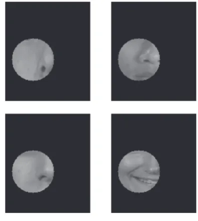
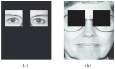
Figure5: Adapting observation distributions: eye/non-eye regions. In this example, eyes, as in (a), have their own observation distribu-tion, built using patch samples from the same regions inS. Likewise, non-eye regions, as in (b), have their own observation distributions, using non-eye regions in the training databaseS.

Figure6: Learned observation clusters withK-means clustering. Shown are the eight regions (K = 8), each represented by a dif-ferent gray-level, of the face learned for this work. The black area represents pixels which do not occur as the center pixel in any patch (cf.Figure 3).

For neighborhood regions, we define a radius distance for each patchi. We then extract patches fromSwhose center co-ordinates in their respective, cropped images fall within that distance (in our case, 32 pixels) from the center pixel ofi. The motivation for this is that patches near a given patch in the face tend to have the same texture.

Alternately, we can tie distributions for patches together so that a group of patches shares the same distribution:

φ−→φG(i), (13)

whereG(i) is the index for the region/group that the patchi belongs to. One simple example of (13) is to separate the face into two regions, as illustrated inFigure 5:

(1) eye region,

(2) other (non-eye region).

We then extract patches fromSwhose center pixels’ coordi-nates fall within the same region as the center pixel of a given patch. One of the motivations for doing this approach over the neighborhood approach is the realization that there are discontinuities in areas that have similar texture, particularly with the eyes.

Finally, patches can be clustered together using machine learning techniques. We useK-means clustering [13] to as-sign each patch to one ofKclusters. One of the reasons for usingK-means clustering is to make the region definitions data-dependent and, hence, better adapted to the actual face data. The clusters are determined by creating long feature vectors of the high-frequency patches across theNtraining images, withQbeing the number of patches extracted from each image (note that there is a shift of only one pixel be-tween patches during the cluster learning):

⎡ ⎢ ⎢ ⎢ ⎢ ⎢ ⎢ ⎣

H1

P[1](:) HP2[1](:) · · · HPN[1](:)

H1

P[2](:) HP2[2](:) · · · HPN[2](:)

..

. ... ... ...

H1

P[Q](:) HP2[Q](:) · · · HPN[Q](:) ⎤ ⎥ ⎥ ⎥ ⎥ ⎥ ⎥ ⎦

, (14)

where each row of (14) is a feature vector input into theK -means and (:) is Matlab notation for the vectorized version of a patch. The result is to find a single clustering fromSand to use this single clustering in enhancing any new face image. In the experiments for this work, we setK =8 (Figure 6), and for eﬃciency reasons, only used a subset ofSfor computing theKregions.

3.3. Adapting transition functionψ

The baselineψ models the transition of a patchionly with the patches bordering it (the patches are referred to as neigh-borhood N(i) of patch i). A given patch i is then (indi-rectly) dependent upon any nonneighboring patch given N(i). However, many of the patches in a face image may be strongly correlated with patches a long distance away. We may therefore want to adapt the definition of N(i) to include long-distance relationships. One type of long-distance “tran-sition” that we can model is related to the vertical line of face symmetry (seeFigure 7). As the face is highly symmetrical, features found on one side of the face will typically be found on the other side of the face. For example, if a person has fa-cial hair on the left side of the face, he will likely also have some on the right side of the face; or someone with freckles on one cheek will also likely have them on the other cheek. For long-distance neighbors, (9) will be modified when com-puting long-distance transitions:

ψi†(i=i,j= j)=exp ⎛ ⎜ ⎝

d†HPn[i],Hn

P [j] 2

σLongTi

⎞ ⎟ ⎠,

(15)

whered†(·) represents the Euclidean distance between the whole of the first patch and the mirror image of the second patch, with an appropriate normalizingσLongTi, as above.

(6)

Figure7: Adapting transition distributions. In this example, three pairs of points are highlighted and connected to illustrate some of the transitions that can be added to a patch’s transition distribution, ψ, therefore, is adapted based on its distance from the vertical line of symmetry in a face.

information between the two is

MI(i,j)=

N

n=1

N

n₌₁

pHPn[i](:),Hn

P[j](:)

·log p

Hn

P[i](:),Hn

P[j](:)

pHn P[i](:)

·pHn

P[j](:) ,

(16)

but with the simplification that p(HPn[i](:),Hn

P[j](:)) = 0

whenn=n, we actually have

MI(i,j)≈

N

n=1

pHPn[i](:),HPn[j](:)

·log p

Hn

P[i](:),HPn[j](:)

pHPn[i](:)

·pHPn[j](:) ,

(17)

where the marginalp(HPn[i](:)) is a single GaussianN(μi,σi2)

with mean and diagonal covariance (denoted using diag(·)), respectively:

μi= N

n=1

Hn P[i](:)

N , (18)

σ2

i =diag _N

n=1

μi−HPn[i](:)

μi−HPn[i](:) T

N−1

. (19)

N(μi,σi2) is normalized such that

1 Ci

N

n=1

pHn P[i](:)

=1. (20)

The jointp(Hn

P[i](:),HPn[j](:)) is defined in a similar way. We

then identify the learned neighbors of each patchIas those with MI(i,j) > δ, where δ is a global threshold. Figure 8 illustrates some of the learned neighborhoods on a sample training face image. The transition betweeniand a learned

Figure8: Learning long-distance dependencies. Shown are exam-ples of the long-distance neighbors for a couple selected patches. In each example, the black patches are in the neighborhood of the sin-gle white patch. In the work in this paper in learning long-distance dependencies, a patch can have between 0 and 30 learned neighbors.

neighbor jis then

ψi††(i=i,j= j)=exp ⎛ ⎜ ⎝

d††HPn[i],Hn

P [j] 2

σLearnedTi

⎞ ⎟ ⎠,

(21)

whered††is the Euclidean distance between the two patches (no mirroring, as done in (15), is performed), with an ap-propriate normalizingσLearnedTi, like before.

4. FACE ENHANCEMENT EXPERIMENTS

4.1. Setup

In this current work, we are assuming that the face has al-ready been located and properly cropped. We have cropped 1151 faces from the “fa” subset of FERET [14],1 _{using the}

eye and nose coordinates provided with the database. As these are high-quality still images and not low-resolution video images, they are useful for investigating how much of the actual high-frequency we can recover. In future work, we can then investigate their performance in more realis-tic environments such as surveillance video (though exam-ples on a “real” low-resolution still image are given below in Figures 12, 13, 14, and 15). 951 faces have been ran-domly extracted for the training set S, while another 100 have been randomly set aside for any tuning of the system

(7)

(a)

(b)

(c)

Figure9: Baseline results. Row (a) contains the target high-resolution image, while rows (b) and (c) present the bicubic interpolation and baseline MRF results, respectively. Compare with Figures10and11.

Table2: Super-resolution of 38×33 pixel images to 150×130 pixels (levelG2to levelG0) showing MSE for the whole image. Results are given using bilinear interpolation, a standard MRF [4], and five of our proposed models: an MRF with observation functions adapted to the region-dependent functions for the eye and non-eye regions; an MRF adapted to the region-dependent functions of neighborhoods; an MRF with observation functions adapted to the region-dependent functions learned usingK-means clustering; an MRF with adapted, symmetrical transitions; and an MRF with long-distance, mutual-information-based transitions. As the various MRFs attempt to further enhance low-resolution images that have already been partially enhanced using bilinear interpolation, the percent reduction (“Red.”) is with respect to bilinear interpolation. The bicubic interpolation MSE is also given for comparison; the MRFs could potentially do even better in future work if they were enhancing images already partially enhanced using bicubic interpolation. Results are from all 100 images in our test set. As the original, high-resolution images are 150×130 pixels each, the 38×33 pixel images were magnified before enhancement by slightly under a factor of four in each dimension; this was done so as to keep all images used in the algorithm the same size.

Baseline MRF 54.3 7.7%

MRF:φG(i)adapted to eye 52.1 11.5%

MRF:φiadapted to neighborhood 50.9 13.6%

MRF:φG(i)adapted usingK-means 53.2 9.7%

MRF:ψiadapted to symmetry 53.7 8.8%

MRF:ψiadapted using mutual info. 64.3 −9.2%

Bicubic interpolation 49.3 16.3%

and the remaining 100 for testing the system. Each image only appears in one of the lists, but, as many of the 694 subjects appear more than once in the database, a subject can appear on more than one list. Each cropped face is, at high resolution, 150×130 pixels. For experimenting with super-resolution, low-resolution versions of these images have also

been produced, as discussed inSection 2.1, by blurring the high-resolution images and subsampling them to produce levelG2of the Gaussian pyramid, which has images of size

38×33.

(8)

(d)

(e)

(f)

Figure10: MRF results: adaptingφ. Row (10(d)) presents results usingφG(i)adapted to the eye regions. Row (10(e)) presents results using φiadapted to neighborhood regions (using a radius around the patch’s center pixel). Row (10(f)) presents results usingφG(i)adapted to regions learned byK-means clustering. Compare with the baseline MRF, which is in row (c) ofFigure 9, and withFigure 11. For the subject in column 1, note, for example, (in comparison with the baseline row (c) inFigure 9) the sharper right eye with a clearer boundary in row (10(e)). For the subject in column 2, note that the left eye in row (10(e)) is shinier. For the subject in column 3, note the more realistic eye and better illuminated cheeks in row (10(e)). For the subject in column 4, note the clearer right eye in row (10(e)) and the better illuminated eye in row (10(f)). For the subject in column 5, note in row (10(f)) both the sharper right eye that is consistent with the left eye and the increased detail in the teeth.

Table3: Super-resolution of 38×33 pixel images to 150×130 pixels (levelG2to levelG0) showing MSE foreyeregion (Figure 5(a)). See

Table 2for additional descriptions of the table.

MRF:ψiadapted using mutual info. 99.7 −4.7%

such investigations, we compare our results with those us-ing the approach of [4], which is also concerned with en-hancing a single image using MRFs. We do not make direct comparisons to approaches, such as [3] or the main results in [7], that utilize multiple images to produce a single re-solved image; this is reserved for future work. Using

infor-Table4: Super-resolution of 38×33 pixel images to 150×130 pixels (levelG2 to levelG0) showing MSE for thenon-eyeregion (Figure 5(b)). SeeTable 2for additional descriptions of the table.

MRF:ψiadapted using mutual info. 52.6 −12.3%

mation only from level 2 of the Gaussian pyramid, we use a baseline MRF from the approach of [4] to infer the high-frequency components missing from the high-resolutionG0

(9)

(g)

(h)

Figure11: MRF results: adaptingψ. Row (11(g)) presents results usingψiadapted using symmetry in the face. Row (11(h)) presents results

usingψi adapted using mutual information of the patches. Compare with the baseline MRF, which is in row (c) ofFigure 9, and with

the MRFs adaptingφinFigure 10. In general, the current methods of adaptingψdo not give as much improvement, by themselves, than adaptingφ.

Figure12: Real low-resolution image, captured by a Canon Power-Shot G5, using the 640×480 resolution mode (only 240×160 pix-els are cut out from the image and shown here) with the extracted faces (cropped with bilinear interpolation in this figure). The super-resolution results are given in Figures13,14, and15for the baseline MRF, the MRFs adapted toφiand toφG(i), and the MRFs adapted to ψi, respectively.

4.2. Results

First, to justify the need for having a full-MRF instead of just local observation functions, we show in Table 1 the diﬀ er-ence that having transition functions also included between neighboring patches provides. By including ψ with φ and having a standard, baseline MRF, we get a mean squared er-ror (MSE) of 54.3. This is an improvement over using either bilinear interpolation orφalone. Given this baseline result using a standard MRF, we then applied our proposed adap-tation techniques. Table 2 gives results of the diﬀerent ap-proaches for enhancing images from G2, that is, those

im-ages which are being enlarged by a factor of approximately 4 in each dimension and then enhanced by super-resolution (note that the MSE values given in this paper do not take into account the unenhanced pixels on the edges of the images,

(b)

(c)

Figure 13: Baseline results on real low-resolution images. Rows (13(b)) and (13(c)) present the bicubic interpolation and base-line MRF results, respectively. To ease comparison with the FERET images of Figure 9, the labeling starts with (13(b)) as no high-resolution images are available.

where no high-resolution patches are placed—seeFigure 3). Here we see that we can, on average, improve the resolution of the face by using MRFs whoseφi,φG(i), orψifunction is

adapted as indicated (with the exception of adaptingψiusing

(10)

(d)

(e)

(f)

Figure 14: Adaptive MRF results on real low-resolution images. Row (14(d)) presents results usingφG(i)adapted to the eye regions. Row (14(e)) presents results usingφiadapted to neighborhood

re-gions (using a radius around the patch’s center pixel). Row (14(f)) presents results usingφG(i)adapted to regions learned byK-means clustering. Compare with the baseline MRF, which is in row (13(c)) ofFigure 13, and withFigure 15.

its neighborhood, which reduced the MSE of bilinear inter-polation by 13.6%, as opposed to just 7.7% for the baseline MRF. As this method takes patches fromSbased only upon their distance between their coordinates and the coordinates of the patch being enhanced, this is one of our simpler adap-tation techniques. While simple, this technique proves eﬀ ec-tive in doing example-based super-resolution in a region-dependent manner.

Figures9,10, and11give the baseline results, results for adaptingφi, and the results for adaptingψi, respectively, for

some of the images that benefited from the adaptation tech-niques (any improvements typically came from adaptingφi

andφG(i) instead of adaptingψi). While subjective, the best

enhanced image for each of the subjects inFigure 10is of-ten that of row (10(e)), which are the outputs of adaptive MRFs withφiadapted to its neighborhood; this is also the

adaptive MRF that performed best quantitatively inTable 2.

(a)

(b)

Figure 15: Adaptive MRF results on real low-resolution images. Row (15(a)) presents results usingψiadapted using symmetry in

the face. Row (15(b)) presents results usingψiadapted using

mu-tual information of the patches. Compare with the baseline MRF, which is in row (13(c)) ofFigure 13and withFigure 14.

Furthermore, even though they are not tailored specifically to eye/non-eye regions, they also do better when looking specif-ically at these regions. As the visual improvements are often in the eye regions, we examined the MSE in the images look-ing only at pixels in the eye regions and also at pixels only in the non-eye regions (as defined byFigure 5, see Tables3and 4).Table 3shows how the modest improvements ofTable 2 become even better when looking specifically at the eyes. This could possibly be due to the MRF’s concentrating at model-ing high-frequency information and to the eyes’ containmodel-ing some of the highest-frequency information in the face (see, e.g.,Figure 2(d)).Table 4shows that the non-eye region of the face, typically with lower-frequency information, bene-fits less from an adaptive MRF.

In addition to the qualitative results shown in Figures 9,10, and 11and the related quantitative results shown in Tables 2, 3, and 4, we also tested our algorithm on real low-resolution images (i.e., those not generated from high-resolution images). Some results are shown in Figures 12, 13,14, and15. The quality of these enhanced images could potentially be improved through using a training setSthat better matches their domain (e.g., using images with outdoor lighting forS).

5. CONCLUSION

(11)

available for the super-resolution; we showed how doing so not only reduces the MSE associated with a standard MRF but how using such adaptation can produce sharper images.

The next steps in this work of adapting MRFs include im-proving the modeling of whereφi,φG(i), andψiare adapted

using machine learning techniques. While using K-means clustering produced acceptable results in adaptingφG(i),

us-ing mutual information in adaptus-ingψican hurt the

resolu-tion. The reason for this may lie, in part, in how the adapted ψiis defined in (21), which is based on the Euclidean distance

between the learned, long-distance neighbors. As the mutual information was based on the joint distributionp(Hn

P[i](:),

Hn

P[j](:)) (and not on their distance) in (17), it may be more

appropriate to use this joint distribution for computingψi.

ACKNOWLEDGMENTS

This research was supported by funding from the IC Postdoc-toral Research Fellowship Program. The anonymous review-ers as well as Datong Chen, David Liu, Simon Lucey, Kate Shim, Ted Square, and Wende Zhang were also of assistance in this research.

REFERENCES

[1] A. K. Jain,Fundamentals of Digital Image Processing, Prentice-Hall, Englewood Cliﬀs, NJ, USA, 1989.

[2] R. Y. Tsai and T. S. Huang, “Multiframe image restoration and registration,” inAdvances in Computer Vision and Image Pro-cessing, vol. 1, chapter 7, pp. 317–339, JAI Press, Greenwich, Conn, USA, 1984.

[3] R. R. Schultz and R. L. Stevenson, “Extraction of high-resolution frames from video sequences,”IEEE Transactions on Image Processing, vol. 5, no. 6, pp. 996–1011, 1996.

[4] W. T. Freeman, E. C. Pasztor, and O. T. Carmichael, “Learn-ing low-level vision,”International Journal of Computer Vision, vol. 40, no. 1, pp. 25–47, 2000.

[5] S. Z. Li,Markov Random Field Modeling in Image Analysis, vol. 19 ofComputer Science Workbench Series, Springer, Tokyo, Japan, 2001.

[6] J. Pearl,Probabilistic Reasoning in Intelligent Systems: Networks of Plausible Inference, Morgan Kaufmann, San Fransisco, Calif, USA, 1988.

[7] S. Baker and T. Kanade, “Limits on super-resolution and how to break them,”IEEE Transactions on Pattern Analysis and Ma-chine Intelligence, vol. 24, no. 9, pp. 1167–1183, 2002. [8] G. Dedeo˘glu, T. Kanade, and J. August, “High-zoom video

hal-lucination by exploiting spatio-temporal regularities,” in Pro-ceedings of IEEE Computer Society Conference on Computer Vi-sion and Pattern Recognition (CVPR ’04), vol. 2, pp. 151–158, Washington, DC, USA, June–July 2004.

[9] S. L. Lauritzen,Graphical Models, Oxford Statistical Science Series, No. 17, Clarendon Press, Oxford, UK, 1996.

[10] H. W. Schneiderman,A statistical approach to 3D object detec-tion applied to faces and cars, Ph.D. thesis, Robotics Institute, Carnegie Mellon University, Pittsburgh, Pa, USA, May 2000, CMU-RI-TR-00-06.

[11] W. T. Freeman, T. R. Jones, and E. C. Pasztor, “Example-based super-resolution,”IEEE Computer Graphics and Applications, vol. 22, no. 2, pp. 56–65, 2002.

[12] J. S. Yedidia, W. T. Freeman, and Y. Weiss, “Generalized be-lief propagation,” inProceedings of Advances in Neural Infor-mation Processing Systems 13 (NIPS ’00), T. K. Leen, T. G. Di-etterich, and V. Tresp, Eds., vol. 13, pp. 689–695, MIT Press, Cambridge, Mass, USA, 2001.

[13] C. M. Bishop,Neural Networks for Pattern Recognition, Oxford University Press, Oxford, UK, 1995.

[14] P. J. Phillips, H. Moon, S. A. Rizvi, and P. J. Rauss, “The FERET evaluation methodology for face-recognition algo-rithms,”IEEE Transactions on Pattern Analysis and Machine In-telligence, vol. 22, no. 10, pp. 1090–1104, 2000.

Todd A. Stephensonhas been a Senior Sci-entist at ReallaeR, LLC, of Saint Leonard, Maryland, since November 2005. From April 2004 to November 2005 he was a Postdoctoral Fellow at the Advanced Multi-media Processing Laboratory, Department of Electrical and Computer Engineering, Carnegie Mellon University, Pittsburgh, Pennsylvania. From March 1999 to June 2003 he was a Research Assistant in the

speech processing group of the IDIAP Research Institute in Mar-tigny, Switzerland. From June 1995 to August 1997 he worked in the Consumer Markets Division of AT&T Corporation in Piscataway, New Jersey, and in Somerset, New Jersey. Todd received the Ph.D. degree in electrical engineering from the Swiss Federal Institute of Technology Lausanne (EPFL) in 2003, the M.S. degree in cognitive science and natural language from the University of Edinburgh in 1998, and the B.S. degree in Mathematics from the Pennsylvania State University in 1995. His research interests include computer vision, machine learning, speech recognition, and natural language processing. He is a Member of the IEEE.

Tsuhan Chen has been with the Depart-ment of Electrical and Computer Engi-neering, Carnegie Mellon University, Pitts-burgh, Pennsylvania, since October 1997, where he is currently a Professor. He directs the Advanced Multimedia Processing Labo-ratory, working on multimedia signal pro-cessing, biometrics, computer vision, and computer graphics. From August 1993 to October 1997, he worked at AT&T Bell