A computationally efficient algorithm for characterizing the superposition of multiple heterogeneous interrupted Bernoulli processes

A

Computationally Efficient

Algorithm for Characterizing the

Superposition of Multiple

Heterogeneous Interrupted

Bernoulli Processes

K. M.

Elsayed

H.

G. Perras

Center for Communications and Signal Processing

Department of Computer Science

"North Carolina State University

/TR-94j14

A

COlnputationally Efficient

Algorithm

for

Characterizing the Superposition of Multiple

Heterogeneous Interrupted Bernoulli Processes

*

Khaled M. Elsayed

Harry G. Perros

Department of Computer Science

and

Center for Communications and Signal Processing

North Carolina State University

Raleigh, NC 27695-8207

June 10, 1994

Abstract

A computationally efficient algorithm for characterizing the superposition process of N heterogeneous and independent Interrupted Bernoulli Processes isintroduced. The algorithm is then used to analyze a statistical multiplexer with finite buffer. Finally, numerical examples highlighting the algorithm accuracy are given.

"Supported in partbyBelJSouth, GTE Corporation, and NSF and DARPA under cooperative agreement

1

Introductioll

In an ATM environment many types of traffic, such as voice, data, and video, are to be

efficiently transported by the same network. An ATM mulliplexer receives cells (fixed size

packets of 53 octets length) from a number of different incoming links and then transmits

them out onto a single outgoing link. A finile buffer is provided in the multiplexer to

accomodate the multiple arrivals of cells. Each arrival stream is modeled by a bursty and

possibly a correlated process. The service time is deterministic and is equal to one slot of

the outgoing link which is assumed to be long enough to transmit one cell.

The analysis of such a queueing system is quite complex due to the large number of

arrival processes. A possible method for approximately analyzing the queue is to first

characterize the superposition process of all arrival prrocesses, and then analysze the

queue with a single arrival process. In this paper, we consider the case when the arrival

processes are modeled as multiple independent heterogeneous Interrupted Bernoulli

Pro-cesses (IBP). The IBP and its variants are popular models for bursty traffic sources in an

ATM environment.

The problem of characterizing the superposition process of a set of arrival processes has

been addressed extensively in the literature. One approach for obtaining the superposition

process is to approximate it by a renewal process, see Albin [1], Whitt [16], Sriram and

Whitt [12], and also Perros and Onvural [11]. An insightful discussion of the various

time-scales affecting the accuracy of the approximate superposition of packet voice sources

(modeled as a variant of IBP) was provided in [12]. Heffes and Lucantoni [6]considered

the superposition process of packet voice sources modeled as an IBP where arrivals occur periodically. They approximate the superposition by a Markov Modulated Poisson

Process (MMPP). The accuracy of the superposition is reasonable when the average delay

in the multiplexer is the amount of paramount importance. However, the superposition

does not provide a good estimate for the probability of loss. Several other authors (see [3,

10, 15]) considered the same problem and suggested alternative methods for characterizing

the superposition process as an MMPP. The main objective of these papers was to improve

the accuracy with regards to calculation of the cell loss probability. Heffes [5] obtained an

MMPP

approximation to the superposition of different MMPP arrival processes using a

Allalternative method to model ATM multiplexers is the Uniform Arrival and Service

(VAS) model (also known as fluid flow). In this case an on/ off process produces a uniform

flow of bits when in the all slate. Cell departures are modeled as a uniform flow out of

the queue. Anick, Mitra, and Sondhi [2] evaluated the system performance using elegant

simple expressions for a multiplexer with infinite buffer space and homogeneous arrivals.

Tucker[14] considered the finite buffer case. TIle methodology was generalized to tile case

of heterogneous Markov Modulated Rate Processes illa series of papers [13, 4].

The work presented ill this paper is related to the methodology presented Hong, Perros,

and Yamashita [7] and Makharnreh, McDonald and Ceorganas [9]. In [7], the authors used

an aggregation method for approximating the superposition process. They first obtained

the exact probability transition matrix of the Markov chain of the superposition process.

This Markov chain has a dimension which is exponential in the number of input sources.

Subsequently, the Markov chain was aggregated in order to obtain a superposition process

with a small number of states (linear function of the number of sources). The method

is limited to a small number of input sources. In [9], the authors used an aggregation

method to analyze an output-buffered ATM switch with correlated imbalanced traffic.

In this paper, we present an efficient algorithm for characterizing the superposition

process of multiple heterogeneous IBP's. The algorithm is based on a step-wise

aggrega-tion scheme. It can be used to construct the superposiaggrega-tion of a large number of IBP sources.

The space complexity of the algorithm is O(N), while the computational complexity is

O(N4 ), where N is the number of superimposed IBP's. TIle superposition algorithm is

then used to study the performance of a statistical multiplexer with finite buffer. Finally,

we present a brief study of the range of parameters of the superimposed IBPs for which

the accuracy of the algorithm is acceptable.

The rest of this paper is organized as follows. In section 2, we briefly describe the IBP

model and discuss some of its statistical properties. III section 3, we discuss the step-wise

aggregation algorithm for characterizing the superposition process. Section 4 presents

the analysis of the statistical multiplexer and numerical results and a discussion of the

Figure 1: TIle Interrupted Bernoulli Process.

2

The

IBP Source Model

We consider a source that alternates between active and idle states according to a Markov

chain (see figure 1). Arrivals occur in a Bernoulli fashion with probability 1 only when

the source is ill the active state. No arrivals occur when the source is in the idle state. The

transitions between active and idle states occur in a mernoryless fashion. Let us assume

that at the end of slot k the process is in the active (or idle) state. Then, in the next slot

k

+

1 it will remain in the active (or idle) state with probability a (or (3), or it will change

to idle (or active) state with probability 1 - a (or 1 - (3).

The inter-arrival time mean

I

and coefficient of variation CV2are givell by:

t =

(1 - a)

+

(1 -

(3),

CV2

=

1

+

I [ (1 - a)(a

+

(3)

-

1].

,(I -

(3)

[(1 - a)

+

(1 - (3)]2

The triplet

(Q,

(J,,) completely characterizes an IBP process.

3

The

Approximation Algorithm

We now present an efficient algorithm that can be used to characterize the superposition

of N ~ 2 heterogeneous IBP sources. We assume that the sources can be divided into G

groups, where the sources within each group are identical. In practice, specially when N

is large, this assumption is valid because traffic sources of a specific traffic type (e.g. data

or voice source) would tend to have similar or even identical characteristics. TIle number

of sources in groupi is given by

Ni,

where 1 ~ N, ~ Nand

L

N,

=

N.

ap-proximation algorithm is to characterize the superposition of sources in group i, where

N,

>

I, in terms of a stochastic process with N,

+

1 states. The superposition process is

described in terms of the probability transition matrix between the N

+

1states, and the

probability distribution of the number of arrivals per slot at each state.

The superposition process of N similar!BP'

s

with descriptor

(0',

f3,,)

is a Markov chain

with state spaceX

=

{n,n

=

0, 1, · · ·N} which denotes the number of sources in the active

state (or alternatively in the idle state). Let A

=

[a(nJ,n2)), nl, n2 E X be the probability

transition matrix governing the transitions between the states of the superposition. Also,

let

b(

n,i) be the probability that i arrivals occur when the superposition is in staten, where

o

~ i ~ n. Consider two states nj and n2. Assume that in slot k the Markov chain is

in state nt· The probability that in tile next slot k

+

I, the Markov chain would be in

state n2 is equal to the probability that I,0 ~ I ~ nI, of the nI sources in the active state

make a transition to idle state and thatm, 0 ~ m ~ N - nl, of the sources in the idle

state make a transition to active state, and that nl - I

+

m

=

»»

The probability of the

first event to occur is given by the binomial distribution (~I)(1

-

O')'O'n

l-'.

Similarly, the

probability that the second event occurs is given by (n~~~~,)(1-

f3t2-nl+'f3N-n2-'

where

o

S

n2 - nl

+

l

S

N - nt and N - n2 - I

2::

o.

We then have:

a(nl,n2)

=

Lr~o [(~I)(1

-

O')'O'n

l-'

(n~~7~,)(1-

f3t2-nl+'f3N-n2-'

I(n2 -

nJ

+

I

:2

0) I(N -

»:-I

:2

O)J

where

I(

x)

==

1 iff logical expression

x

is true and 0 otherwise.

When there are n sources each with probability f of emitting a cell in a given slot,

the the probability of having v arrivals is given by the binomial distribution b(n, v)

==

(:),v(1 -

f

)n-v,

0

~

v

~

n. For notational convenience, the quantities

b(

n,

v)

are referred

to by the lower triangular matrix B == [b(n, v)].

11-The Combined Superposition Process of two Groups of Sources:Oncethe superpo-sition of two or more separate groups of sources is constructed as described above, itis

necessary to combine them in order to get the overall superposition process. Let us as-sume that the superposition process of two arbitrary groups, say groups 1 and 2, has been

where n; is the state of component process i. The number of states in the superposition

process is equal to (N]

+

1)(N2

+

1). The probability transition matrix of the superposition

will be givell by A == A10 A2where 0 is tile Kroencker product operation of two matrices.

One of theuseful properties of the Kroencker product operation is thatif,the invariant

probability vector of A,is givell by

7rl

®

7f2

where

ii

is invariant probability vector of Ai.

This saves us from solving a system of linear equations for finding the invariant of P

which is more time consuming than solving for

7ft

and

7f2

individually.

Note that the above discussion is also valid for more than two groups of sources.

However, we focus here on the case of two groups since the approximation algorithm always superposes two processes at a time.

111-Aggregation of the Superposition Process: TIle above Markov chain which

charac-terizes the superposition process of two groups of IBP sources is exact. However, the

dimensionality of the resulting process may not be practical for studying the performance

of amultiplexer with alarge buffer. The dimensionality of the superposition process can

be reduced by lumping all thest~tes (nl'n2)of thesuperposition, wherenl

+

n2

==

n, to a single state n. The Markov chain resulting from this aggregation represents what we call

the

compact

superposition process.

Let the probability transition matrix of the compact process be

A

=

[ii(n, m)]' We then

have

The remaining step is to find the probability distribution function of the number of

arrivals in a particular state. This can be calculated from Bi ,i

=

1,2as follows:

(2)

The resulting superposition process has a characterization identical to that of its

IV-The Approximation Algorithm: Consider N heterogeneous IBP sources divided

into G groups each having Ni,i

=

1,2" · ·G, identical sources. Then, we have the

algo-rithm outline as follows:

oFind Aj , ifj andB, for all grollps j, j == 1,··.,G

o Let Aa == Al and B/J == ill

oForj

==

2 toG do

o A' == A/J ® Aj

-II -I -I

01r ==1r/J0 7rj

o Aggregate A' into A,(use equation 1)

o Calculate B/J (use equation2)

o Find1r/J satisfying1f/JA/J == i/J'

Ei

-rr/J(i) == 1

End

It can be shown that the computational complexity of the algorithm is O(N4 ) (The

calculation of the Kroencker product of two matrices and the solution of a linear system

of equations are the dominant factors.)

Hong, Perros, and Yamashita [7] tackled the same problem. However, their proposed

algorithm constructs the complete probability transition matrix of the superposition

pro-cess and then performs the aggregation. This causes tile computational complexity and

storage requirements of their method to be O(2N ) . This precludes the execution of the

algorithm on a conventional computer. Even for a nominal value ofN, sayN

==

20, it may

not be possible to construct the superposition even using a supercomputer. Our method

has the same accuracy but it is considerably more efficient.

4

Analysis of the Multiplexer Model

Consider a FIFO finite buffer multiplexer servingN ~ 2 IBP sources as depicted in figure 2.

The multiplexer has S

2

1 servers and can accommodate a total of B ~ S cells at any time

instant including those in service. The service time for all cells is constant and is equal to

o

SI

~

0

S2~

•

.

SN~ _{Finite Buffcr Queue (B-S)}

Traffic Sources

0

I Slot Service (S Servers)

Figure 2: The Statistical Multiplexer with Sservers and B total waiting capacity.

State Transition

/ArriVal

---1

I

k /k+l

Service Completion

k+2 _k+3

Time Slot

Figure 3: Timing of events in the early arrival model.

otherwise no queue will ever form in the multiplexer and the problem will be trivial to handle.

We seek the steady state probabilities, 1r(n), 0 ~ n ~ B - S, that there are n cells in

the multiplexer's queue. From this, we can obtain other measures of interest such as the

mean queue length, the probability of full buffer and the cell loss probability.

Let us first discuss the timing of events ill our system. We follow an

early arrival

timing model as defined by Hunt [8]. That is, during all arbitrary time slot, the following

sequence of events is possible: potential state transition in the superposition occurs,

followed immediately by cell arrivals (if any), which is followed by service of waiting

cells if there are any, and finally departure of cells that received service. This is shown

in figure 3. If an arbitrary cell sees one or more empty servers UpOll its arrival, it is

immediately admitted to one of the available servers without waiting till the next slot.

Hence, the multiplexer is effectively of the cut-through type.

The system state is described by the pair

(n, h)

where

n

is the number of customers

process at the current slot.

We first characterize the superposition process of the N IBP sources as described in

the previous section. Then, the probability transition matrix of the Markov chain (n,

h)

is generated. Let p[(nl,hI) ---+ (n2,h 2)] be the probability that the Markov Chain (n,h)

makes a transition from state

(nt, hJ)

in slot kto state_{(n2, h2)}in slotk

+

1.Then

v

wheren2

=

(min( nl

+

v), B) -

st

andv,0 ~ v ~ hI,is the random variable representing

the number of arrivals when the superposition process is in state h-: Finally, we solve

for the invariant probability vector of P

=

[p[(nl,hJ) ---+ (n2,h2)]] from which various

performance metrics can be obtained. We used the Gauss-Seidel method when using a

workstation, and the parallelized LAPACK routines for LU decomposition when using a KSR-l parallel machine at the NorthCarolina SupercomputerCenter.

5

Validation and Numerical Examples

The approximation algorithm was validated bycomparingitagainst simulation. The effect of the heterogeneity of the sources on the accuracy of the algorithm was investigated and metrics were defined to determine how heterogeneous a given set of sources is. These metrics can be used to determine in advance whether the superposition will be accurate or not.

In all the validation examples, we fixIi, the probability that sourcej emits a cell while in the active state, to be 1. This simplifies the fitting procedure for characterizing an IBP

from the first two moments of the inter-arrival time. TIle following additional notation is used.

Pi= Source throughput for a source in group i.

R_p

=

max{Pi} /min{Pi} is ameasure of heterogeneity of the throughput of the input sources.

Rcu2

=

_max{CVi2}jmin{Cl/?}_{is a measure of heterogeneity of the CV}2_{of the input sources.}

A

=

I:f=l

Nio,

= Total throughput.

B

=

Total buffer size.

In all examples, the number of serversill the multiplexerwas set to 1.

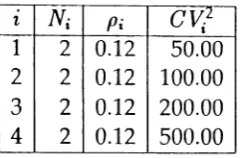
Example 1: In the first example, we have G == 4 and B == 24 and we use the input

sources with parameters given in table 1.

1, N· _Pi CV2

I _I

1 2 0.12 50.00

2 2 0.12 100.00

3 2 0.12 200.00

4 2 0.12 500.00

Table 1: Parameters for the first example.

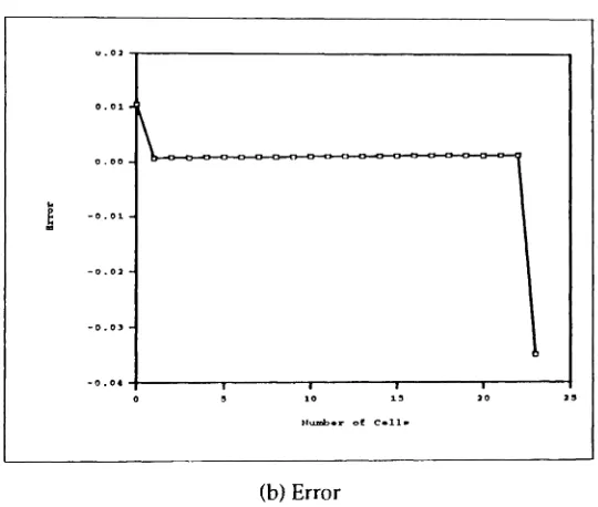
In figure 4(a), we plot the distribution of the number of cells in the queue which is

obtained from simulation and the approximation algorithm. The difference between the

numerical and simulation values is shown in figure 4(b). The reason why we give the

difference and not the relative error is that some of the calculated quantities are very small

(in the order of 10-3) which makes the relative error to be large, despite the fact that the

overall accuracy is still acceptable. The probability distribution has two peaks, the first

is for the probability that queue is full and the second peak for the probability that the

queue is empty. This a well-knownbehavior ill queues with bursty correlated input with

a moderate to a high input traffic intensity. We note that the magnitude of error of the

steady-state probability of a full buffer is high, This causes an underestimation of the

cell loss probability. However, it should be stated thatfor this example theinput sources

are quite heterogeneous. The value of Rcv2is 10, which is fairly large as it will be shown

below.

Example2: In the second example, we use the inputsources with parameters given in

table 2, withR_{cv 2} == 4. We first obtain the superposition process, and subsequently use it to

generate the probability transition matrix for buffer sizes in the set {10,20,30,40,50,60, 70}.

The cell loss probability and the mean queue length are shown in figures 5(a) and 5(b)

0.5

O ••

t 0.]

-~ ~ ~

0.1

0.0

I

5

I

10

I

15

- j

I

:10

- 0 -AnAlytio • • -0 . . .81mulation

(a) Probability distribution of the number of cells

0.01

-0.02

- 0 . 0 '

l

-0.ot~ - - ~ - - - r - - - r - - - - f

1~

)lumb.r of C . l l .

(b) Error

Figure 4: Probability distribution of the number of cells and associated error, B

==

24.

I . _N

i I Pi

cvl

1- I

1 2 0.1 10.00 2 2 0.1 20.00 3 2 0.1 30.00

4 2 0.1 40.00

good while that of the cell loss probability is less accurate. This is due to the smoothing

effect of the aggregation algorithm. It constructs a less bursty and correlated process than

the actual superposition, which leads to underestimating the probability of observing a

full buffer. However, we noted that the aggregation algorithm provides an upper-bound

on the probability of having an empty buffer. Thus a balancing effect takes place and the

overall meanqueue length predicted by the simulation and numerical solution is close.

We also investigated the effect of increasing the Humber of sources in a group while

keeping the overall grollp throughput fixed. TIle parameters of table 2were modified as

follows. N, is increased to 4, Pi is halved to 0.05, for all i == 1",·,4 and the values of

Clii

remained the same. For this new set of parameters, the probability of loss and mean

queue length slightly increased over the values plotted in figure 5. The accuracy remained

the same.

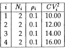
Example 3: The third example is in essence similar to the second one. We letRcv 2

==

1.6

and the parameters of the input sources are given by table 3.

The probability of loss and the mean queue length are shown in figures 6(a) and 6(b)

respectively. We note here that the accuracy of the approximation algorithm is very good.

This is due to the fact that the amount of heterogeneity in the input sources is small as

indicated by the relatively small value of Rcv 2 .

t N_{i Pi}

ev?

₁

1 2 0.1 10.00

2 2 0.1 12.00

3 2 0.1 14.00

4 2 0.1 16.00

Table 3: Parameters for the third example.

We also conducted a set of experiments to study the effect of the variation in IBP source

throughput and coefficient of variation on the accuracy of the approximation algorithm.

We know in advance that the more heterogeneous the sources are, the worse the accuracy

of the iterative aggregation algorithm would become. However, we wanted to find out

the regions for the parameters of the sources in which the accuracy of the algorithm

is acceptable. The conclusion of this study was that Rcv2 is a major deciding factor in

I---~--- - - - . - - - _

- 0 -I\n'-lI;-I:ICI'lI • • -0 • • •Sjmul'-Itie-n

~,

\

...

••

_'~""

",

"l:l

<,

.. '0 ...

.... 0 O. 20

I-~---u.15

!II .~

~ u. 10 .Q f

u.05

0.00- r - - - r - - - r - - y - - - , r - - - - , . - - - J

10 20 )0 40 SO 60 70 80

(a) Probability of loss

2 0 . , - - - _

15

!II .-f

~ ~

~ 10

§

~

~ ):

- - - 0 - - -Analyt ic • • -0 • • •Sim.Jletion

10 20 )0 40 50 60 70 80

Buf r",r slz"

(b) Mean number of cells

o.~O. , - - - - _

o15

~ 0.10 .0

~

o05

- - - 0 . -I\na IytIr~l

•• -0 . . .SimulatIon

u .00-r--r--~-r---..,r----,.---I

10 20 )0 40 50 60 70 80

Bufr~[" slz~

(a) Probability of loss

16

1tI

12 {II

..-4 ..-4 ~ ~ 10

'-t

.8

~

c:

~ 1I

~

10 20 )0 40 50 60 70 80 B'J [r4>r S17,.,

(b) Mean number of cells

- - 0 - -I\nalyticl')}

• • -0 • • •Simulation

Example 4: In this example, we discuss the effect of the variation in the squared

coef-ficient of variation of the inter-arrival time of the input sources on the accuracy. We

con-structed an input of four groups each having two sources, and fixed the source throughput

to be0.1. We vary the Rc tJ2 to take values from the set {I, 1.5,2,2.5,3,3.5,4,4.5,5}

respec-tively. We assume that

ell?

=

10.0,and for each value of

R

c tJ2 , we find the remaining

ev?

by solving the following eqllalions:

cv

2

ev~

=

(J, i

=

2,3,4

1-1

where () is set equal to

\I

Rcu 2 •

We plotted the cell loss probability, obtained from the approximation algorithm and

simulation, and the percentile error as a function of Rcv 2 in figures 7(a) and 7(b)

respec-tively. We note that the relative error is an increasing pseudo-linear function of Reu2 • We

observed that in general if Rcv 2

>

3, then the approximation algorithm does not perform

satisfactorily. This seems to hold true independent of the maximum or minimum values

of C~2. In some cases, the accuracy actually improves when the minimum and maximum value of the C~2 are increased, while keeping the value of Rcu2 fixed. This may be in contrast to what one would initially conjecture that the larger the absolute values of C~2 the worse the algorithm would perform.

Example 5: In this example, we discuss the effect of variation in the throughput of the

inputsources, We consider four groups of sources each having a single source. The total

throughput is fixed at 0.8 and each source has a squared coefficient of variation equal to

20. We let

R;

take values from the set {l, 10,20,30,40,50}. The throughput of a single

sourcepi,i

==

1,· · ·4 is calcula ted by solving

4

~

=

(J,i

=

2,3,4,

L

Pi

=

0.8

Pi-l i=l

where0 =

fi4.

We plotted the cell loss probability, obtained from the approximation algorithm and

simulation, and the percentile error as a function of

R;

in figures 8(a) and 8(b) respectively.

throughput by many orders of magnitude than Ole coefficient of variation. Even for very

large values of Rp , say 40, tile relative error is about 100/0. In addition, we have observed

that the algorithm becomes less sensitive to R; when there are more than one source in a

g~vengroup. In other words, the case of one source per group is an extreme case in which the effect of heterogeneity in tile throughput of the input sources is large.

6

Concl

USiOllS

A computationally efficient algorithm for characterizing the superposition process of

multiple possibly-heterogeneous groups of IBP sources was introduced. Tile accuracy of

the algorithm depends to a large extent on the degree of heterogeneity of the sources. We

found out that a good measure of the heterogeneity of the sources is the ratio of the largest

to the smallest coefficient of variation of tile inter-arrival time. This ratio can be used to

forecast the accuracy of the algorithm without the need to conlpare with simulation. A

good rule of thumb is to use the algorithm for cases when this ratio is in the range

[0,2.5].

This, however, still needs further testing for large buffer sizes and under various ratios

between the buffer size and the largest average on period of the sources (note that this

ratio plays a major role in affecting system performance.)

An interesting study would be to compare our method with other approaches that

characterize the superposition process as a 2-state MMPP, e.g. the work in [3, 10, 15]. We

plan to use the results of this model in studying call admission control and comparing the

different methodologies and bounds available in the literature.

References

[1] S. L. Albin. Approximating a point process by a renewal process, 2: Superposition

of arrival processes to queues.

Operations Research,

32:1133-1162, 1984.

[2] D. Anick, D. Mitra, and M. M. Sondhi. Stochastic theory of a data-handling system

0 . 0 8 , - - _

0.06

III

.3

~

g

0.04

~_.o ~

0.02

- G -1\nolytic • • -0 • • •slmulfttlon

0.00-.---y----r__--_----J

(a) Probability of loss

35

25

20

1 S

10

»>:

.>

~

/

V

/

.}/

7

V

(b) Percentile relative error

- - - .

u.045

0.010

III

.3 _0.0)5

~

g

I

0 0)0 0.025

0.020 ,,

.".

.

",

....Q" ....

....

...

-''''-- -''''-- -''''-- 0 -''''-- -''''--I\nl!lllyt 1c

• • -0 • • •sim.Jletion

10 20 )0 4 0 so

15.0

12.5

10.0

s .0

2.5

(a) Probability of loss

---- ---.

/

/

/

-:

./

V

/

10 20 30 40 50

(b) Percentile relative error

[3] A. Baiocchi, N. B. Melazzi, M. Listani, A. Roveri, and R. Winkler. Loss Performance

Analysis of an ATM Multiplexer Loaded with High-Speed On-Off Sources.

IEEE

Journal on Selected Areas in Communications,

9:388-393, 1991.

[4] A.I.Elwalid, D. Mitra, andT.E. Stern. Statistical multiplexing of Markov modulated

sources: Theory and computational algorithms. In

Proceedings of 13th International

Teletraffic Congress,

pages 495-500, Copenhagen, June 1991.

[5] H. Heffes. A class of data traffic process: covariance function characterization and

related queueing results.

Bell Sys. Tech.

j., 59:897-929, 1980.

[6] H. Heffes and D. M. Lucantoni. A Markov Modulated Characterization of Packetized

Voice and Data Traffic and Related Statistical Multiplexer Performance.

IEEE Journal

on Selected Areas in Communications,

4:856-867, 1986.

[7] S. Hong, H. G. Perros, and H. Yamashita. A discrete-time queueing model of the

shared buffer ATM switch with bursty arrivals.

Telecommunication Systems,

2:1-20,

1993.

[8] J. Hunter.

Mathematical Techniques ofApplied Probability. Volume

2:

Discrete Time Models:

Techniques and Applications,

chapter 9. Academic Press, 1983.

[9] I. I. Makhamreh, D. McDonald, and N. D. Georganas. Aanlysis of an Output-Buffered ATM Switch with Imbedded Bursty Traffic. Submitted for publication, 1994.

[10] R.Nagarajan,

J.

F.Kurose, and D. Towsley. Approximation Techniques for Computing

Packet Loss in Finite-Buffered Voice Multiplexers. IEEE

Journal on Selected Areas

ill

Communications,

9:368-377, 1991.

[11] H. G. Perros and R. Onvural. On the superposition of arrival processes for voice

and data. In

Fourth International Conference

011

Data Communication Syste1ns and Their

Performance,

pages 341-357, Barcelona, June 1990.

[12] K. Sriram and W. Whitt. Characterizing Superposition Arrival Processes in Packet

Multiplexers for Voice and Data.

IEEE Journal

011

Selected Areas in Communications,

6:833-846, 1986.

[13] T. E. Stern and A. I. Elwalid. Analysis of separable Markov-modulated rate models

for information-handling systems.

Adv. Appl. Prob.,

23:105-139, 1991.

[14] R. C. F. Tucker. Accurate method for analysis of a packet-speech multiplexer with

limited delay.

IEEE Transactions on Communications,

36:479-483, 1988.

[15] S. S. Wang and

J.

A. Silvester. A Fast Performance Model for Real-Time Multimedia

Communication. In

Proceedings of the Fifth International Conference on Data

Communi-cation Systems and Their Performance,

Raleigh, NC, October 1993.

[16] W. Whitt. Approximation of a point process by a renewal process, 1: Two basic