Kernel Affine Projection Algorithms

Volume 2008, Article ID 784292,12pages doi:10.1155/2008/784292

Research Article

Kernel Affine Projection Algorithms

Weifeng Liu and Jos ´e C. Pr´ıncipe

Department of Electrical and Computer Engineering, University of Florida, Gainesville, FL 32611, USA

Correspondence should be addressed to Weifeng Liu,[email protected]

Received 27 September 2007; Revised 23 January 2008; Accepted 21 February 2008

Recommended by An´ıbal Figueiras-Vidal

The combination of the famed kernel trick and affine projection algorithms (APAs) yields powerful nonlinear extensions, named collectively here, KAPA. This paper is a follow-up study of the recently introduced kernel least-mean-square algorithm (KLMS). KAPA inherits the simplicity and online nature of KLMS while reducing its gradient noise, boosting performance. More interestingly, it provides a unifying model for several neural network techniques, including kernel least-mean-square algorithms, kernel adaline, sliding-window kernel recursive-least squares (KRLS), and regularization networks. Therefore, many insights can be gained into the basic relations among them and the tradeoffbetween computation complexity and performance. Several simulations illustrate its wide applicability.

Copyright © 2008 W. Liu and J. C. Pr´ıncipe. This is an open access article distributed under the Creative Commons Attribution License, which permits unrestricted use, distribution, and reproduction in any medium, provided the original work is properly cited.

1. INTRODUCTION

The solid mathematical foundation, wide and successful applications are making kernel methods very popular. By the famed kernel trick, many linear methods have been recast in high dimensional reproducing kernel Hilbert spaces (RKHS) to yield more powerful nonlinear extensions, including support vector machines [1], principal component analysis [2], recursive least squares [3], Hebbian algorithm [4], Adaline [5], and so forth.

More recently, a kernelized least-mean-square (KLMS) algorithm was proposed in [6], which implicitly creates a growing radial basis function network (RBF) with a learning strategy similar to resource-allocating networks (RAN) proposed by Platt [7]. As an improvement, kernelized affine projection algorithms (KAPAs) are presented for the first time in this paper by reformulating the conventional affine projection algorithm (APA) [8] in general reproducing kernel Hilbert spaces (RKHS). The new algorithms are online, simple, and significantly reduce the gradient noise compared with the KLMS and thus improve performance.

More interestingly, the KAPA reduces to the kernel least-mean square (KLMS), sliding-window kernel recursive least squares (SW-KRLS), kernel adaline, and regularization networks naturally in special cases. Thus it provides a unifying model for these existing methods and helps better understand the basic relations among them and the tradeoff

between complexity and performance. Moreover, it also advances our understanding on the resource-allocating net-works. Exploiting the underlying linear structure of RKHS, a brief discussion on its well-posedness will be conducted.

The organization of the paper is as follows. InSection 2, the affine projection algorithms are briefly reviewed. Next, in Section 3, the kernel trick is applied to formulate the non-linear affine projection algorithms. Other related algorithms are reviewed as special cases of the KAPA inSection 4. We detail the implementation of the KAPA inSection 5. Three experiments are studied inSection 6to support our theory. Finally, Section 7 summarizes the conclusions and future lines of research.

The notation used throughout the paper is summarized inTable 1.

2. A REVIEW OF THE AFFINE PROJECTION ALGORITHMS

Let d be a zero-mean scalar-valued random variable, and let u be a zero-mean L × 1 random variable with a positive-definite covariance matrixRu=E

uuT_{. The}

cross-covariance vector ofdanduis denoted byrdu=E

du. The weight vectorwthat solves

min

w Ed−w

T_u2 ₍₁₎

Several methods that approximatewiteratively also exist, for example, the common gradient method

w(0)=initial guess;

w(i)=w(i−1) +ηrdu−Ruw(i−1)

, (2)

or the regularized Newton’s recursion

w(0)=initial guess;

w(i)=w(i−1) +ηRu+εI −1

rdu−Ruw(i−1)

, (3)

whereεis a small positive regularization factor andηis the step size specified by the designer.

Stochastic-gradient algorithms replace the covariance matrix and the cross-covariance vector by local approx-imations directly from data at each iteration. There are several ways for obtaining such approximations. The tradeoff is computation complexity, convergence performance, and steady-state behavior [8].

Assume that we have access to observations of the random variablesdanduover time

d(1),d(2),. . ., u(1),u(2),. . .. (4)

The Least-mean-square (LMS) algorithm simply uses the instantaneous values for approximationsRu=u(i)u(i)Tand rdu=d(i)u(i). The corresponding steepest-descent recursion (2) and Newton’s recursion (3) become

w(i)=w(i−1) +ηu(i)d(i)−u(i)Tw(i−1);

w(i)=w(i−1)+ηu(i)u(i)Tu(i)+εI−1d(i)−u(i)Tw(i−1).

(5)

The affine projection algorithm however employs better approximations. Specifically, Ru and rdu are replaced by the instantaneous approximations from the K most recent regressors and observations. Denoting

U(i)=u(i−K+ 1),. . .,u(i)_L×K,

d(i)=d(i−K+ 1),. . .,d(i)T,

(6)

one has

Ru= 1

KU(i)U(i) T

,

rdu= 1

KU(i)d(i).

(7)

Therefore, (2) and (3) become

w(i)=w(i−1) +ηU(i)d(i)−U(i)Tw(i−1), (8)

w(i)=w(i−1)+ηU(i)U(i)T+εI−1U(i)d(i)−U(i)Tw(i−1), (9)

and (9), by the matrix inversion lemma, is equivalent to [8]

w(i)=w(i−1) +ηU(i)U(i)TU(i) +εI−1

×d(i)−U(i)Tw(i−1).

(10)

Table1: Notations.

Description Examples Scalars Smallitalicletters d Vectors Smallboldletters w,ω,a

Matrices CapitalBOLDletters U,Φ

Time or iteration Indices in parentheses u(i),d(i) Components of vectors

or matrices Subscript indices aj(i),Gi,j

It is noted that this equivalence lets us deal with the matrix

U(i)TU(i)+εIinstead ofU(i)U(i)T+εIand it plays a very important role in the derivation of kernel extensions. We call recursion (8) APA-1 and recursion (10) APA-2.

In some circumstances, a regularized solution is needed instead of (1). The regularized LS problem is

min

w Ed−w

T_u2_+λw2_{, (11)}

whereλis the regularization parameter (not the regulariza-tion factorεin Newton’s recursion). The gradient method is

w(i)=w(i−1) +ηrdu−

λI+Ru

w(i−1)

=(1−ηλ)w(i−1) +ηrdu−Ruw(i−1)

. (12)

The Newton’s recursion withε=0 is

w(i)=w(i−1) +ηλI+Ru −1

rdu−(λI+Ru)w(i−1)

=(1−η)w(i−1) +ηλI+Ru −1

rdu.

(13)

If the approximations (7) are used, we have

w(i)=(1−ηλ)w(i−1) +ηU(i)d(i)−U(i)Tw(i−1), (14)

w(i)=(1−η)w(i−1) +ηλI+U(i)U(i)T−1U(i)d(i).

(15)

which is, by the matrix inversion lemma, equivalent to

w(i)=(1−η)w(i−1) +ηU(i)λI+U(i)TU(i)−1d(i).

(16)

For simplicity, recursions (14) and (16) are named here APA-3 and APA-4, respectively.

3. THE KERNEL AFFINE PROJECTION ALGORITHMS

A kernel [9] is a continuous, symmetric, positive-definite function κ : U ×U → R. U is the input domain, a compact subset ofRL_{. The commonly used kernels include}

the Gaussian kernel (17) and the polynomial kernel (18):

κ(u,u)=exp−au−u2

, (17)

κ(u,u)=uT_{u+ 1}p

The Mercer theorem [9,10] states that any kernelκ(u,u) can be expanded as follows:

κ(u,u)= ∞

i=1

σiφi(u)φi(u), (19)

whereσiandφiare the eigenvalues and the eigenfunctions,

respectively. The eigenvalues are nonnegative. Therefore, a mappingϕcan be constructed as

ϕ:U−→F,

ϕ(u)=√σ1φ1(u),√σ2φ2(u),. . .

,

(20)

such that

κ(u,u)=ϕ(u)Tϕ(u). (21)

By construction, the dimensionality ofFis determined by the number of strictly positive eigenvalues, which can be infinite in the Gaussian kernel case.

We utilize this theorem to transform the datau(i) into the feature space F as ϕ(u(i)) and interpret (21) as the usual dot product. Denotingϕ(i) = ϕ(u(i)), we formulate the affine projection algorithms on the example sequence {d(1),d(2),. . .}and{ϕ(1),ϕ(2),. . .}to estimate the weight vectorωthat solves

min

ω Ed−ω

T_ϕ(u)2_{. (22)}

By straightforward manipulation, (8) becomes

ω(i)=ω(i−1) +ηΦ(i)d(i)−Φ(i)Tω(i−1), (23)

and (10) becomes

ω(i)=ω(i−1) +ηΦ(i)Φ(i)TΦ(i) +εI−1

×d(i)−Φ(i)Tω(i−1),

(24)

whereΦ(i)=ϕ(i−K+ 1),. . .,ϕ(i). Accordingly, (14) becomes

ω(i)=(1−λη)ω(i−1) +ηΦ(i)d(i)−Φ(i)Tω(i−1), (25)

and (16) becomes

ω(i)=(1−η)ω(i−1) +ηΦ(i)Φ(i)TΦ(i) +λI−1d(i).

(26)

For simplicity, we refer to the recursions (23), (24), (25), and (26) as KAPA-1, KAPA-2, KAPA-3, and KAPA-4, respectively.

3.1. Kernel affine projection algorithm (KAPA-1)

It may be difficult to have direct access to the weights and the transformed data in feature space, so (23) needs to be

modified. If we set the initial guessω(0)=0, the iteration of (23) will be

ω(0)=0,

ω(1)=ηd(1)ϕ(1)=a1(1)ϕ(1),

.. .

ω(i−1)=

i−1

j=1

aj(i−1)ϕ(j),

Φ(i)Tω(i−1)= _i−1

j=1

aj(i−1)κi−K+1,j,. . .,

i−1

j=1

aj(i−1)κi−1,j, i−1

j=1

aj(i−1)κi,j

T

,

e(i)=d(i)−Φ(i)Tω(i−1),

ω(i)=ω(i−1) +ηΦ(i)e(i)

=

i−1

j=1

aj(i−1)ϕ(j) + K

j=1

ηej(i)ϕ(i−j+K),

(27)

whereκi,j=κ(u(i),u(j)) for simplicity.

Note that during the iteration, the weight vector in the feature space assumes the following expansion:

ω(i)=

i

j=1

aj(i)ϕ(j) ∀i >0, (28)

that is, the weight at timei is a linear combination of the previous transformed input. This result may seem simply a restatement of the representer theorem in [11]. However, it should be emphasized that this result does not rely on any explicit minimal norm constraint as required for the representer theorem. As pointed out in [12], the gradient search in (28) has an inherent regularization mechanism which guarantees the solution is in the data subspace under appropriate initialization. In general, the initializationω(0) can introduce whatever apriori information is available, which can be any linear combination of any transformed data in order to utilize the kernel trick.

By (28), the updating on the weight vector reduces to the updating on the expansion coefficients

ak(i)=

⎧ ⎪ ⎪ ⎪ ⎪ ⎪ ⎪ ⎪ ⎪ ⎪ ⎪ ⎪ ⎪ ⎪ ⎪ ⎨ ⎪ ⎪ ⎪ ⎪ ⎪ ⎪ ⎪ ⎪ ⎪ ⎪ ⎪ ⎪ ⎪ ⎪ ⎩

η

d(i)−

i−1

j=1

aj(i−1)κi,j

, k=i,

ak(i−1) +η

d(k)−

i−1

j=1

aj(i−1)κk,j

,

i−K+ 1≤k≤i−1,

ak(i−1), 1≤k < i−K+ 1.

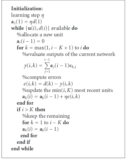
Initialization: learning stepη

a1(1)=ηd(1)

while{u(i),d(i)}availabledo

%allocate a new unit

ai(i−1)=0

fork=max(1,i−K+ 1) toido

%evaluate outputs of the current network

y(i,k)=

i−1

j=1

aj(i−1)κk,j

%compute errors e(i,k)=d(k)−y(i,k)

%update the min(i,K) most recent units

ak(i)=ak(i−1) +ηe(i,k)

end for ifi > Kthen

%keep the remaining

fork=1 toi−Kdo ak(i)=ak(i−1)

end for end if end while

Algorithm1: Kernel affine projection algorithm (KAPA-1).

Sinceei+1−k(i) = d(k)− i−1

j=1

aj(i−1)κk,j is the prediction

error of data {u(k),d(k)} by the network ω(i − 1), the interpretation of (29) is straightforward: allocate a new unit with coefficient ηe1(i) and update the coefficients for the otherK−1 most recent units byηei+1−k(i) fori−K+ 1 ≤ k≤i−1.

The pseudocode for KAPA-1 is listed inAlgorithm 1.

3.2. Normalized KAPA (KAPA-2)

Similarly, the regularized Newton’s recursion (24) can be factorized into the following steps:

ω(i−1)=

i−1

j=1

aj(i−1)ϕ(j),

e(i)=d(i)−Φ(i)Tω(i−1),

G(i)=Φ(i)TΦ(i),

ω(i)=ω(i−1) +ηΦ(i)G(i) +εI−1e(i).

(30)

In practice, we do not have access to the transformed weight ωor any transformed data, so the update has to be on the expansion coefficientalike in KAPA-1. The whole recursion is similar to the KAPA-1 except that the error is normalized by aK×KmatrixG(i) +εI−1.

3.3. Leaky KAPA (KAPA-3)

The feature space may be infinite dimensional depending on the chosen kernel, which may cause the cost function (22) to

be ill posed in the conventional empirical risk minimization (ERM) sense [13]. The common practice is to constrain the solution norm:

min

ω Ed−ω

T_ϕ(u)2_+λω2_{. (31)}

As we have already shown in (25), the leaky KAPA is

ω(i)=(1−λη)ω(i−1) +ηΦ(i)d(i)−Φ(i)Tω(i−1).

(32)

Again, the iteration will be on the expansion coefficient a, which is similar to the KAPA-1:

ak(i)=

⎧ ⎪ ⎪ ⎪ ⎪ ⎪ ⎪ ⎪ ⎪ ⎪ ⎪ ⎪ ⎪ ⎪ ⎪ ⎨ ⎪ ⎪ ⎪ ⎪ ⎪ ⎪ ⎪ ⎪ ⎪ ⎪ ⎪ ⎪ ⎪ ⎪ ⎩

η

d(i)−

i−1

j=1

aj(i−1)κi,j

, k=i,

(1−λη)ak(i−1) +η

d(k)−

i−1

j=1

aj(i−1)κk,j

,

i−K+ 1≤k≤i−1,

(1−λη)ak(i−1), 1≤k < i−K+ 1.

(33)

The only difference is that KAPA-3 has a scaling factor (1−

λη) multiplying the previous weight, which is usually less than 1, and it imposes a forgetting mechanism so that the training data in the far past are scaled down exponentially. Furthermore, since the network size is growing over training, any transformed data can be pruned from the expansion easily if its coefficient is smaller than some prespecified threshold. For large data sets, the growing nature of this fam-ily of algorithms poses a big problem for implementations, therefore, network size control is very important. We will discuss this issue more in the sparsification section.

3.4. Leaky KAPA with Newton’s recursion (KAPA-4)

As before, the KAPA-4 (26) reduces to

ak(i)=

⎧ ⎪ ⎪ ⎪ ⎪ ⎪ ⎪ ⎪ ⎪ ⎨ ⎪ ⎪ ⎪ ⎪ ⎪ ⎪ ⎪ ⎪ ⎩

ηd(i), k=i,

(1−η)ak(i−1) +ηd(k),

i−K+ 1≤k≤i−1,

(1−η)ak(i−1), 1≤k < i−K+ 1.

(34)

Among these four algorithms, the first three require the error information to update the network which is computationally expensive. Therefore, the different update rule in KAPA-4 has a huge significance in terms of computation since it only needs aK×Kmatrix inversion, which, by using the sliding-window trick, only requiresO(K2_{) operations [14].}

Table2: Comparison of four KAPA update rules.

Algorithm Update equation

KAPA-1 ω(i)=ω(i−1) +ηΦ(i)[d(i)−Φ(i)Tω(i−1)] KAPA-2 ω(i)=ω(i−1) +ηΦ(i)[Φ(i)

T

Φ(i) +εI]−1[d(i)−

Φ(i)Tω(i−1)]

KAPA-3 ω(i)=(1−λη)ω(i−1)+ηΦ(i)[d(i)−Φ(i)Tω(i−1)] KAPA-4 ω(i)=(1−η)ω(i−1)+ηΦ(i)[Φ(i)TΦ(i)+λI]−1d(i)

4. A TAXONOMY FOR RELATED ALGORITHMS

4.1. Kernel least-mean-square algorithm (KAPA-1,K=1)

IfK=1, KAPA-1 reduces to the following kernel least-mean-square algorithm (KLMS) introduced in [6]:

ω(i)=ω(i−1) +ηϕ(i)d(i)−ϕ(i)Tω(i−1). (35)

It is not difficult to verify that the weight vector assumes the following expansion:

ω(i)=

i

j=1

e(j)ϕ(j), (36)

wheree(j)=d(j)−ω(j−1)Tϕ(j) is the apriori error. It is seen that the KLMS allocates a new unit when a new training data comes in with the inputu(i) as the center and the prediction error as the coefficient (scaled by the step size). In other words, once the unit is allocated, the coefficient is fixed. It mimics the resource-allocating step in the RAN algorithm whereas it neglects the adaptation step. In this sense, the KAPA algorithms, that allocate a new unit for the present input and also adapt the other K−1 most recent allocated units, are closer to the original RAN.

The normalized version of the KLMS is as follows (NKLMS):

ω(i)=ω(i−1) + ηϕ(i)

ε+κi,i

d(i)−ϕ(i)Tω(i−1), (37)

Notice that for translation invariant kernels, that is, κi,i =

const, the KLMS is automatically normalized. Sometimes we use KLMS-1 and KLMS-2 to distinguish the two.

4.2. Norma (KAPA-3,K=1)

Similarly, the KAPA-3 (25) reduces to the Norma algorithm introduced by Kivinen in [15]:

ω(i)=(1−ηλ)ω(i−1) +ηϕ(i)d(i)−ϕ(i)Tω(i−1).

(38)

4.3. Kernel Adaline (KAPA-1,K=N)

Assume that the size of the training data is finiteN. If we set

K=N, then the update rule of the KAPA-1 becomes

ω(i)=ω(i−1) +ηΦd−ΦTω(i−1), (39)

where the full data matrices are

Φ=ϕ(1),. . .,ϕ(N), d=d(1),. . .,d(N). (40)

It is easy to check that the weight vector also assumes the following expansion:

ω(i)=

N

j=1

aj(i)ϕ(j), (41)

and the updating on the expansion coefficients is

aj(i)=aj(i−1) +η

d(j)−ϕ(j)Tω(i−1). (42)

This is nothing but the kernel adaline introduced in [5]. Notice the fact that the kernel adaline is not an online method.

4.4. Recursively adapted radial basis function networks (KAPA-3,ηλ=1,K=N)

Assume the size of the training data isNas above. If we set

ηλ=1 andK=N, the update rule of KAPA-3 becomes

ω(i)=ηΦd−ΦTω(i−1), (43)

which is the recursively adapted RBF (RA-RBF) network introduced in [16]. This is a very intriguing algorithm using the “global” error directly to compose the new network. By contrast, the KLMS-1 uses the apriori errors to compose the network.

4.5. Sliding-window Kernel RLS (KAPA-4,η=1)

In KAPA-4, if we setη=1, we have

ω(i)=Φ(i)Φ(i)TΦ(i) +λI−1d(i), (44)

which is the sliding-window kernel RLS (SW-KRLS) intro-duced in [14]. The inverse operation of the sliding-window Gram matrix can be simplified toO(K2_).

4.6. Regularization networks (KAPA-4,η=1,K=N)

We assume there are only N training data and K = N. Equation (26) becomes directly

ω(i)=ΦΦTΦ+λI−1d, (45)

which is the regularization network (RegNet) [13].

We summarize all the related algorithms inTable 3 for convenience.

5. KAPA IMPLEMENTATION

Table3: List of related algorithms.

Algorithm Update equation Relation to KAPA KLMS ω(i)=ω(i−1) +ηϕ(i)[d(i)−ϕ(i)Tω(i−1)] KAPA-1,K=1

NKLMS ω(i)=ω(i−1) + ηϕ(i) (ε+κi,i)

[d(i)−ϕ(i)Tω(i−1)] KAPA-2,K=1

Norma ω(i)=(1−ηλ)ω(i−1) +ηϕ(i)[d(i)−ϕ(i)Tω(i−1)] KAPA-3,K=1 Kernel Adaline ω(i)=ω(i−1) +ηΦ[d−ΦT_{ω(i−1)] KAPA-1,K=N}

RA-RBF ω(i)=ηΦ[d−ΦTω(i−1)] KAPA-3,ηλ=1,K=N SW-KRLS ω(i)=Φ(i)[Φ(i)TΦ(i) +λI]−1d(i) KAPA-4,η=1 RegNet ω(i)=Φ[ΦT_Φ+λI]−1_{d KAPA-4,η=1,K=N}

5.1. Error reusing

As we see in KAPA-1, KAPA-2, and KAPA-3, the most time-consuming part of the computation is to obtain the error information. For example, supposeω(i−1) = i−1

j=1aj(i−

1)ϕ(j). We need to calculatee(i,k)=d(k)−ω(i−1)Tϕ(k) (i−K + 1 ≤ k ≤ i) to computeω(i), which consists of (i−1)Kkernel evaluations. Asiincreases, this dominates the computation time. In this sense, the computation complexity of the KAPA isKtimes of the KLMS. However, after a careful manipulation, we can shrink the complexity gap between KAPA and the KLMS.

Assume that we store all theKerrorse(i−1,k)=d(k)− ω(i−2)Tϕ(k) for i−K ≤ k ≤ i−1 from the previous iteration. At the present iteration, we have

e(i,k)=d(k)−ϕ(k)Tω(i−1)

=d(k)−ϕ(k)Tω(i−2) +η i−1

j=i−K

e(i−1,j)ϕ(j)

=d(k)−ϕ(k)Tω(i−2)+η i−1

j=i−K

e(i−1,j)κj,k

=e(i−1,k) +

i−1

j=i−K

ηe(i−1,j)κj,k.

(46)

Since e(i −1,i) has not been computed yet, we have to calculate e(i,i) by i −1 times kernel evaluation anyway. Overall the computation complexity of the KAPA-1 isO(i+

K2_{), which isO(K}2_{) more than the KLMS.}

5.2. Sliding-window gram matrix inversion

In KAPA-2 and KAPA-4, another computation difficulty is to invert aK×K matrix, which normally requiresO(K3_). However, in the KAPA, the data matrixΦ(i) has a sliding window structure, therefore, a trick can be used to speed up the computation. The trick is based on the matrix inversion formula and was introduced in [14]. We outline the basic

calculation steps here. Suppose the sliding matrices share the same sub-matrixD:

G(i−1) +λI= ⎡ ⎣a bT

b D ⎤

⎦_{, G(i) +λI=} ⎡ ⎣D h

hT _g

⎤ ⎦_,

(47)

and we know from the previous iteration that

G(i−1) +λI−1= ⎡ ⎣e fT

f H ⎤

⎦_{. (48)}

First, we need to calculate the inverse ofDas

D−1=H−ffT_{/e. (49)}

Then, we can update the inverse of the new Gram matrix as

G(i) +λI−1= ⎡

⎣D−1+ (D−1h)(D−1h)

T_{s −}

(D−1_h)s

−(D−1_h)T_{s s} ⎤ ⎦

(50)

withs = (g−hT_D−1_h)−1_.s−1 _{is the Schur complement of} Din (G(i) +λI), which actually measures the distance of the new data to the otherK−1 most recent data in the feature space. The overall complexity isO(K2_).

5.3. Sparsification

is the cardinality. When a new data pair{u(i+ 1),d(i+ 1)}is presented, a decision is made immediately whetheru(i+ 1) should be added into the dictionary as a center.

The novelty criterion introduced by Platt is relatively simple. First, it calculates the distance ofu(i+1) to the present dictionary dis1 = mincj∈D(i)u(i+ 1)−cj. If it is smaller

than some preset threshold, sayδ1,u(i+ 1) will not be added into the dictionary. Otherwise, the method computes the prediction errore(i+ 1,i+ 1)=d(i+ 1)−ϕ(i+ 1)Tω(i). Only if the prediction error is larger than another preset threshold, sayδ2,u(i+ 1) will be accepted as a new center.

The ALD test introduced in [3] is more computationally involved. It tests the following cost dis2 = min∀bϕ(u(i+ 1))−cj∈D(i)bjϕ(cj)which indicates the distance of the

new input to the linear span of the present dictionary in the feature space. It turns out that dis2is the Schur complement of the Gram matrix of the present dictionary. As we saw in the previous section, this result can be used to get the new Gram matrix inverse ifu(i+1) is accepted into the dictionary. Therefore, this method is more suitable for the KAPA-2 and KAPA-4 because of efficiency. This link is very interesting since it reveals that the ALD test actually guarantees the invertibility of the new Gram matrix.

In the sparse model, if the new data is determined to be “novel,” theK−1 most recent data points in the dictionary are used to form the data matrixΦ(i) together with the new data. Therefore, a new unit is allocated and the update is on theK−1 most recent units in the dictionary. If the new data is determined to be not “novel,” it is simply discarded in this paper, but a different strategy can be employed to utilize the information like in [3,7].

The important consequences of the sparsification proce-dure are as follows.

(1) If the input domainUis a compact set, the cardinality of the dictionary is always finite and upper bounded. This statement is not hard to prove using the finite covering theorem of the compact set and the fact that elements in the dictionary are δ-separable [3]. Here is the brief idea: suppose spheres with diameter δ are used to cover U and the optimal covering number is N. Then, because any two centers in the dictionary can not be in the same sphere, the total number of the centers will be no greater thanN

regardless of the distribution and temporal structure ofu. Of course, this is a worst case upper bound. In the case of finite training data, the network size will be finite anyway. This is true in applications like channel equalization, where the training sequence is part of each transmission frame. In a stationary environment, the network converges quickly and the threshold on prediction errors plays its part to constrain the network size. We will validate this claim in the simulation section. In a nonstationary environment, more sophisticated pruning methods should be used to constrain the network size. Simple strategies include pruning the oldest unit in the dictionary [14], pruning randomly [17], and pruning the unit with the least coefficient or similar [18,19]. Another alternative approach is to solve the problem in the primal space [20, 21] directly by using the low rank approximation methods such as Nystr¨om method [22],

Table4: Performance comparison in MG time series prediction.

Algorithm Parameters Test mean square error LMS η=0.04 0.0208±0.0009 KLMS η=0.02 0.0052±0.00022 SW-KRLS K=50,λ=0.1 0.0052±0.00026 KAPA-1 η=0.03,K=10 0.0048±0.00023 KAPA-2 η=0.03,K=10,ε=0.1 0.0040±0.00028 KRLS λ=0.1 0.0027±0.00009

incomplete Cholesky factorization [23], and kernel principal component analysis [2]. It should be pointed out that the scalability issue is at the core of the kernel methods and so all the kernel methods need to deal with it in one way or the other. Indeed, the sequential nature of the KAPA enables active learning [24,25] on huge data sets which is impossible in batch mode algorithms like regularization networks. The discussion on active learning with the KAPA is out of the scope of this paper and will be part of the future work.

(2) Based on (1), we can prove that the solution norms of KLMS-1 and KAPA-1 are upper bounded [12].

The significance of (1) is of practical interest because it states that the system complexity is controlled by the novelty criterion parameters, and designers can estimate a worst case upper bound. The significance of (2) is of theoretical interest because it guarantees the well-posedness of the algorithms. The well-posedness of the KAPA-3 and KAPA-4 is mostly ensured by the regularization term, see [13,14] for details.

6. SIMULATIONS

6.1. Time series prediction

The first example is the short-term prediction of the Mackey-Glass (MG) chaotic time series [26,27]. It is generated from the following time delay ordinary differential equation:

dx(t)

dt = −bx(t) +

ax(t−τ)

1 +x(t−τ)10, (51)

with b = 0.1, a = 0.2, and τ = 30. The time series is discretized at a sampling period of 6 seconds. The time embedding is 7, that is,u(i)=x(i−7),x(i−6),. . .,x(i−1)T are used as the input to predict the present onex(i) which is the desired response here. A segment of 500 samples is used as the training data and another 100 points as the test data (in the testing phase, the filter is fixed). All the data is corrupted by Gaussian noise with zero mean and 0.001 variance.

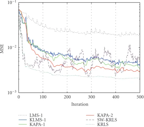
We compare the prediction performance of KLMS, KAPA-1, KAPA-2, KRLS, and a linear combiner trained with LMS. A Gaussian kernel with kernel parametera=1 in (17) is chosen for all the kernel-based algorithms. One hundred Monte Carlo simulations are run with different realizations of noise. The results are summarized inTable 4.Figure 1is the learning curves for the LMS, KLMS-1, 1, KAPA-2 (K =10), and KRLS, respectively. As expected, the KAPA outperforms the KLMS.

Iteration

0 100 200 300 400 500

10−3 10−2 10−1

MSE

LMS-1 KLMS-1 KAPA-1

KAPA-2 SW-KRLS KRLS

Figure1: The learning curves of the LMS, KLMS, KAPA-1 (K =

10), KAPA-2 (K=10), SW-KRLS (K=50), and KRLS.

Table5: Complexity comparison at iterationi.

Algorithm Computation Memory

LMS O(L) O(L)

KLMS O(i) O(i)

SW-KRLS O(K2_{) O(K}2₎ KAPA-1 O(i+K2_{) O(i+K)}

KAPA-2 O(i+K2_{) O(i+K}2₎

KAPA-4 O(K2_{) O(i+K}2₎ KRLS O(i2_{) O(i}2₎

the tables are in the form of “average±standard deviation.” Table 5 summarizes the computational complexity of these algorithms. The KLMS and KAPA effectively reduce the com-putational complexity and memory storage when compared with the KRLS. KAPA-3 and sliding-window KRLS are also tested on this problem. It is observed that the performance of the KAPA-3 is similar to KAPA-1 when the forgetting term is very close to 1 as expected, and the results are severely biased when the forgetting term is reduced further. The reason can be found in [12]. The performance of the sliding-window KRLS is included inFigure 1andTable 4withK =50. It is observed that KAPA-4 (including the sliding-window KRLS) does not perform well with smallK(<50).

Next, we test how the novelty criterion affects the performance. A segment of 1000 samples is used as the training data and another 100 as the test data. All the data is corrupted by Gaussian noise with zero mean and 0.001 variance. The thresholds in the novelty criterion are set as

δ1 = 0.02 and δ2 = 0.06. The learning curves are shown inFigure 2and the results are summarized inTable 6. It is seen that the complexity can be reduced dramatically with the novelty criterion with slight performance degeneration.

Iteration

0 200 400 600 800 1000

0 200 400 600 800 1000

0 200 400 600 800 1000

10−4 10−2 10−0 10−3 10−2 10−1 10−3 10−2 10−1

MSE

KLMS

KAPA-2 KAPA-1

Non-sparse Sparse

Figure2: The learning curves of the KLMS-1, KAPA-1 (K =10),

and KAPA-2 (K=10) with and without sparsification.

Here, SKLMS and SKAPA denote the sparse KLMS and the sparse KAPA, respectively.

Several comments follow: although formally being adap-tive filters, these algorithms can be viewed as efficient alternatives to batch mode RBF networks; therefore, it is practical to freeze their weights during the test phase. Moreover, when compared with other nonlinear filters such as RBF’s, we divide the data in training and testing as normally done in neural networks. Of course, it is also feasible to use the apriori prediction error as a performance indicator like in conventional adaptive filtering literature.

6.2. Noise cancellation

Another important problem in signal processing is noise cancellation in which an unknown interference has to be removed based on some reference measurement. The basic structure of a noise cancellation system is shown inFigure 3. The primary signal is s(i) and its noisy measurementd(i) acts as the desired signal of the system. n(i) is a white noise process which is unknown, and u(i) is its reference measurement, that is, a distorted version of the noise process through some distortion function, which is unknown in general. Here, u(i) is the input of the adaptive filter. The objective is to useu(i) as the input to the filter and to obtain, as the filter output, an estimate of the noise source n(i). Therefore, the noise can be subtracted fromd(i) to improve the signal-noise ratio.

In this example, the noise source is assumed white, uniformly distributed between [−0.5, 0.5]. The interference distortion function is assumed to be

u(i)=n(i)−0.2u(i−1)−u(i−1)n(i−1)

Table6: Performance comparison in MG time series prediction on novelty criterion.

Algorithm Parameters Test mean square error Dictionary size KLMS-1 η=0.02 0.0015±0.00012 1000 SKLMS-1 η=0.02 0.0021±0.00017 220 KAPA-1 η=0.03 0.0012±0.00014 1000 SKAPA-1 η=0.03 0.0017±0.00016 209 KAPA-2 η=0.03,=0.1 0.0007±0.00010 1000 SKAPA-2 η=0.03,=0.1 0.0011±0.00016 195

Noise source

Primary signal

Interference distortion function:H(•)

Primary signal

Adaptive filter n(i)

s(i)

n(i)

u(i)

d(i) y(i) +

+ −

Figure3: The basic structure of the noise cancellation system.

As we see, the distortion function has infinite impulsive response, which, on the other hand, means it is impossible to recovern(i) from a finite time delay embedding ofu(i). We rewrite the distortion function as

n(i)=u(i) + 0.2u(i−1)−0.4u(i−2)

+u(i−1)−0.1n(i−1).

(53)

Therefore, the present value of the noise sourcen(i) depends not only on the reference noise measureu(i),u(i−1),u(i− 2), but also on the previous valuen(i−1), which in turn depends on u(i − 1),u(i −2),u(i − 3), and so on. It means we need a very long time embedding (infinite long theoretically) in order to recovern(i) accurately. However, the recursive nature of the adaptive system provides a feasible alternative, that is, we feedback the output of the filter

n(i−1), which is the estimate ofn(i−1), to estimate the present one, pretendingn(i−1) is the true value ofn(i−1). Therefore, the input of the adaptive filter can be in the form of u(i),u(i−1),u(i −2),n(i −1). It can be seen that the system is inherently recurrent. In the linear case with a DARMA model, it is studied underoutput error methods [28]. However, it will be nontrivial to generalize the results concerning convergence and stability to nonlinear cases, and we will address it in the future work.

We assume the primary signal s(i) = 0 during the training phase. And the system simply tries to reconstruct the noise source from the reference measure. We use a linear filter trained with the normalized LMS, two nonlinear filters trained with the SKLMS-1, and the SKAPA-2 (K = 10), respectively. 2000 training samples are used and 400 Monte Carlo simulations are run to get the ensemble learning curves as shown inFigure 4. The step size and regularization parameter for the NLMS are 0.2 and 0.005. The step sizes for SKLMS-1 and SKAPA-2 are 0.5 and 0.2, respectively.

Iteration

0 500 1000 1500 2000

0 0.01 0.02 0.03 0.04 0.05 0.06

MSE

NLMS SKLMS-1 SKAPA-2

Figure 4: Ensemble learning curves of NLMS, SKLMS-1, and

SKAPA-2 (K=10) in noise cancellation.

Table7: Noise reduction comparison in noise cancellation.

Algorithm Network size NR(dB)

NLMS N/A 9.40

SKLMS-1 581 16.97

SKAPA-2 507 22.99

The Gaussian kernel is used for both KLMS and KAPA with kernel parameter a = 1. The tolerance parameters for KLMS and KAPA are δ1 = 0.15 and δ2 = 0.01, and the noise reduction factor (NR), which is defined as 10log₁₀{En2_{(i)/E[n(i)−y(i)]}2_}

, is listed in Table 7. The performance improvement of SKAPA-2 is obvious when compared with SKLMS-1.

6.3. Nonlinear channel equalization

Linear channelH(z) Nonlinearityf

s(i) x(i)

n(i) r(i) +

+

Figure5: Basic structure of the nonlinear channel.

The problem setting is as follows: a binary signal {s(1),s(2),. . .,s(N)}is fed into the nonlinear channel. At the receiver end of the channel, the signal is further corrupted by additive i.i.d. Gaussian noise and is then observed as {r(1),r(2),. . .,r(N)}. The aim of channel equalization (CE) is to construct an inverse filter that reproduces the original signal with as low an error rate as possible. It is easy to formulate CE as a regression problem, with input-output examples{(r(t+D),r(t+D−1),. . .,r(t+D−l+ 1)),s(t)}, wherelis the time embedding length, andDis the equalization time lag.

In this experiment, the nonlinear channel model is defined byx(t)=s(t)+0.5s(t−1),r(t)=x(t)−0.9x(t)2+n(t), where n(t) is the white Gaussian noise with a variance of

σ2_{. We compare the performance of the LMS1, the APA1,} the SKLMS1, the SKAPA1 (K = 10), and the SKAPA2 (K = 10). The Gaussian kernel with a = 0.1 is used in the SKLMS and SKAPA selected with cross validation.l=3 andD=2 in the equalizer. The noise variance is fixed here

σ =0.1. The learning curve is plotted inFigure 6. The MSE is calculated between the continuous output (before taking the hard decision) and the desired signal. For the SKLMS1, SKAPA1, and SKAPA2, the novelty criterion is employed withδ1 = 0.07,δ2 = 0.08. The incremental growth of the network is also plotted inFigure 7over the training. It can be seen that at the beginning, the network sizes increase quickly, but after convergence, the network sizes increase slowly. And in fact, we can stop adding new centers after convergence by cross-validation by noticing that the MSE does not change after convergence.

Next, different noise variances are set. To make the comparison fair, we tune the novelty criterion parameters to make the network size almost the same (around 100) in each scenario by cross validation. For each setting, 20 Monte Carlo simulations are run with different training data and different testing data. The size of the training data is 1000 and the size of the testing data is 105. The filters are fixed during the testing phase. The results are presented in Figure 8. The normalized signal-noise ratio (SNR) is defined as 10log₁₀(1/σ2_{). It is clearly shown that the} SKAPA-2 outperforms the SKLMS-1 substantially in terms of the bit error rate (BER). The linear methods never really work in this simulation regardless of the SNR. The improvement of the SKAPA-1 on the SKLMS-1 is marginal but it exhibits a smaller variance. The variability in the curves is mostly due to the variance from the stochastic training.

In the last simulation, we test the tracking ability of the proposed methods by introducing an abrupt change during training. The training data is 1500. For the first 500 data, the channel model is kept the same as before, but for the last 1000 data, the nonlinearity of the channel is switched tor(t) = −x(t) + 0.9x(t)2+n(t). The ensemble learning curves from

Iteration

0 2000 4000 6000 8000 10000

0 0.2 0.4 0.6 0.8 1 1.2 1.4

MSE

LMS1 APA1 SKLMS1

SKAPA1 SKAPA2

Figure 6: The learning curves of the LMS1, APA1, SKLMS1,

SKAPA1, and SKAPA2 in the nonlinear channel equalization (σ = 0.1).

Iteration

0 2000 4000 6000 8000 10000

0 20 40 60 80 100 120

Ne

tw

o

rk

si

ze

SKLMS1 SKAPA1 SKAPA2

Figure 7: Network size over training in the nonlinear channel

equalization.

100 Monte Carlo simulations are plotted inFigure 9, and the dynamic change of the network size is plotted inFigure 10. It is seen that the SKAPA-2 outperforms other methods with its fast tracking speed. It is also noted that the network sizes increase right after the change to the channel model.

7. DISCUSSION AND CONCLUSION

Normalized SNR (dB)

0 5 10 15 20 25 30

0 0.05 0.1 0.15 0.2 0.25

BER

LMS1 APA1 SKLMS2

SKAPA1 SKAPA2

Figure 8: Performance comparison with different SNR in the

nonlinear channel equalization.

Iteration

0 500 1000 1500

0 0.2 0.4 0.6 0.8 1 1.2 1.4 1.6 1.8 2

MSE

LMS1 APA1 SKLMS1

SKAPA1 SKAPA2

Figure 9: Ensemble learning curves in the nonlinear channel

equalization with an abrupt change at iteration 5000.

recently introduced KLMS. Since the KAPA update equation can be written as inner products, KAPA can be efficiently computed in the input space. The good approximation ability of the KAPA stems from the fact that the transformed dataϕ(u) includes possibly infinite different features of the original data. In the framework of stochastic projection, the space spanned byϕ(u) is so large that the projection error of the desired signal could be very small [31], as is well known from Cover’s theorem [32]. This capability includes modeling of nonlinear systems, which is the main reason why the KAPA can achieve good performance in the

Mackey-Iteration

0 500 1000 1500

0 20 40 80 60 100 120 140 160

Ne

tw

o

rk

si

ze

SKLMS1 SKAPA1 SKAPA2

Figure 10: Network size over training in the nonlinear channel

equalization with an abrupt change at iteration 500.

Glass system prediction, adaptive noise cancellation, and nonlinear channel equalization.

Comparing with the KLMS, KRLS, and regularization networks (batch mode training), KAPA gives yet another way of calculating the coefficients for shallow RBF like neural networks. The performance of the KAPA is somewhere between the KLMS and KRLS, which is specified by the window lengthK. Therefore, it not only provides a further theoretical understanding of RBF like neural networks, but it also brings much flexibility for application design with the constraints on performance and computation resources.

Three examples are studied in the paper, namely, time series prediction, nonlinear channel equalization, and nonlinear noise cancellation. In all examples, the KAPA demonstrates superior performance when compared with the KLMS, which is expected from the classic adaptive filtering theory.

As pointed out, the study of the KLMS and KAPA has a close relation with the resource-allocating networks, but in the framework of RKHS, any Mercer kernel can be used instead of restricting the architecture to the Gaussian kernel. An important avenue for further research is how to choose the optimal kernel for a specific problem. A lot of work [33–35] has been done in the context of classical machine learning, which is usually derived in a strict optimization manner. Notice that with stochastic gradient methods, the solution obtained is not strictly the optimal solution, therefore, further investigation is warranted. As we mentioned before, how to control the network size is still a big issue, which needs further study.

ACKNOWLEDGMENT

REFERENCES

[1] V. Vapnik,The Nature of Statistical Learning Theory, Springer, New York, NY, USA, 1995.

[2] B. Sch¨olkopf, A. J. Smola, and K.-R. M¨uller, “Nonlinear component analysis as a kernel eigenvalue problem,”Neural Computation, vol. 10, no. 5, pp. 1299–1319, 1998.

[3] Y. Engel, S. Mannor, and R. Meir, “The kernel recursive least-squares algorithm,” IEEE Transactions on Signal Processing, vol. 52, no. 8, pp. 2275–2285, 2004.

[4] K. I. Kim, M. O. Franz, and B. Sch¨olkopf, “Iterative kernel principal component analysis for image modeling,” IEEE Transactions on Pattern Analysis and Machine Intelligence, vol. 27, no. 9, pp. 1351–1366, 2005.

[5] T.-T. Frieb and R. F. Harrison, “A kernel-based adaline,” in Proceedings of the 7th European Symposium on Artificial Neural Networks (ESANN ’99), pp. 245–250, Bruges, Belgium, April 1999.

[6] P. P. Pokharel, W. Liu, and J. C. Pr´ıncipe, “Kernel LMS,” inProceedings of IEEE International Conference on Acoustics, Speech and Signal Processing (ICASSP ’07), vol. 3, pp. 1421– 1424, Honolulu, Hawaii, USA, April 2007.

[7] J. Platt, “A resource-allocating network for function interpola-tion,”Neural Computation, vol. 3, no. 2, pp. 213–225, 1991. [8] A. Sayed,Fundamentals of Adaptive Filtering, John Wiley &

Sons, New York, NY, USA, 2003.

[9] N. Aronszajn, “Theory of reproducing kernels,”Transactions of the American Mathematical Society, vol. 68, no. 3, pp. 337–404, 1950.

[10] C. J. C. Burges, “A tutorial on support vector machines for pattern recognition,”Data Mining and Knowledge Discovery, vol. 2, no. 2, pp. 121–167, 1998.

[11] B. Sch¨olkopf, R. Herbrich, and A. J. Smola, “A generalized representer theorem,” inProceedings of the 14th Annual Con-ference on Computational Learning Theory and 5th European Conference on Computational Learning Theory, pp. 416–426, Amsterdam, The Netherlands, July 2001.

[12] W. Liu, P. P. Pokharel, and J. C. Pr´ıncipe, “The kernel least mean square algorithm,” IEEE Transactions on Signal Processing, vol. 56, no. 2, pp. 543–554, 2008.

[13] F. Girosi, M. Jones, and T. Poggio, “Regularization theory and neural networks architectures,” Neural Computation, vol. 7, no. 2, pp. 219–269, 1995.

[14] S. Van Vaerenbergh, J. V´ıa, and I. Santamar´ıa, “A sliding-window kernel RLS algorithm and its application to nonlin-ear channel identification,” in Proceedings of IEEE Interna-tional Conference on Acoustics, Speech and Signal Processing (ICASSP ’06), vol. 5, pp. 789–792, Toulouse, France, May 2006. [15] J. Kivinen, A. J. Smola, and R. C. Williamson, “Online learning with kernels,”IEEE Transactions on Signal Processing, vol. 52, no. 8, pp. 2165–2176, 2004.

[16] W. Liu, P. P. Pokharel, and J. C. Pr´ıncipe, “Recursively adapted radial basis function networks and its relationship to resource allocating networks and online kernel learning,” inProceedings of IEEE International Workshop on Machine Learning for Signal Processing (MLSP ’07), pp. 300–305, Thessaloniki, Greece, August 2007.

[17] G. Cavallanti, N. Cesa-Bianchi, and C. Gentile, “Tracking the best hyperplane with a simple budget Perceptron,”Machine Learning, vol. 69, no. 2-3, pp. 143–167, 2007.

[18] S. Yonghong, P. Saratchandran, and N. Sundararajan, “A direct link minimal resource allocation network for adaptive noise cancellation,”Neural Processing Letters, vol. 12, no. 3, pp. 255– 265, 2000.

[19] O. Dekel, S. Shalev-Shwartz, and Y. Singer, “The forgetron: a kernel-based perceptron on a fixed budget,” inAdvances in Neural Information Processing Systems 18, pp. 1342–1372, MIT Press, Cambridge, Mass, USA, 2006.

[20] A. Navia-V´azquez, F. P´erez-Cruz, A. Art´es-Rodr´ıguez, and A. R. Figueiras-Vid´al, “Weighted least squares training of support vector classifiers leading to compact and adaptive schemes,” IEEE Transactions on Neural Networks, vol. 12, no. 5, pp. 1047– 1059, 2001.

[21] J. A. K. Suykens, T. V. Gestel, J. D. Brabanter, B. D. Moor, and J. Vandewalle,Least Squares Support Vector Machines, World Scientific, Singapore, 2002.

[22] C. K. I. Williams and M. Seeger, “Using the Nystr¨om method to speed up kernel machines,” inAdvances in Neural Information Processing Systems 13, T. K. Leen, T. G. Dietterich, and V. Tresp, Eds., pp. 682–688, chapter 13, MIT Press, Cambridge, Mass, USA, 2001.

[23] S. Fine and K. Scheinberg, “Efficient svm training using low-rank kernel representations,” Journal of Machine Learning Research, vol. 2, pp. 242–264, 2001.

[24] A. Bordes, S. Ertekin, J. Weston, and L. Bottou, “Fast kernel classifiers with online and active learning,”Journal of Machine Learning Research, vol. 6, pp. 1579–1619, 2005.

[25] K. Fukumizu, “Active learning in multilayer perceptrons,” in Advances in Neural Information Processing Systems 8, D. S. Touretzky, M. C. Mozer, and M. E. Hasselmo, Eds., pp. 295– 301, MIT Press, Cambridge, Mass, USA, 1996.

[26] L. Glass and M. Mackey,From Clocks to Chaos: The Rhythms of Life, Princeton University Press, Princeton, NJ, USA, 1988. [27] S. Mukherjee, E. Osuna, and F. Girosi, “Nonlinear prediction

of chaotic time series using support vector machines,” in Proceedings of the 7th IEEE Workshop on Neural Networks for Signal Processing, J. C. Pr´ıncipe, L. Giles, N. Morgan, and E. Wilson, Eds., pp. 511–520, IEEE Press, Amelia Island, Fla, USA, September 1997.

[28] G. C. Goodwin and K. S. Sin,Adaptive Filtering Prediction and Control, Prentice Hall, Upper Saddle River, NJ, USA, 1984. [29] G. Kechriotis, E. Zervas, and E. S. Manolakos, “Using

recur-rent neural networks for adaptive communication channel equalization,”IEEE Transactions on Neural Networks, vol. 5, no. 2, pp. 267–278, 1994.

[30] N. P. Sands and J. M. Cioffi, “Nonlinear channel models for digital magnetic recording,”IEEE Transactions on Magnetics, vol. 29, no. 6, part 2, pp. 3996–3998, 1993.

[31] E. Parzen, “Statistical methods on time series by hilbert space methods,” Tech. Rep. 23, Applied Mathematics and Statistics Laboratory, Stanford University, Stanford, Calif, USA, 1959. [32] S. Haykin, Neural Networks: A Comprehensive Foundation,

Prentice Hall, Upper Saddle River, NJ, USA, 2nd edition, 1998. [33] C. A. Micchelli and M. Pontil, “Learning the kernel function via regularization,” Journal of Machine Learning Research, vol. 6, pp. 1099–1125, 2005.

[34] A. Argyriou, C. A. Micchelli, and M. Pontil, “Learning convex combinations of continuously parameterized basic kernels,” in Proceedings of the18th Annual Conference on Computational Learning Theory (COLT ’05), pp. 338–352, Bertinoro, Italy, June 2005.