Characterizing Image Sets Using
Formal Concept Analysis
Emmanuel Zenou
National School of Aeronautics and Space (SUPAERO), 10 Edouard Belin Avenue, BP 54032, 31055 Toulouse Cedex, France
LAAS -CNRS, 7 Colonel Roche Avenue, 31077 Toulouse Cedex 4, France Email:[email protected]
Manuel Samuelides
National School of Aeronautics and Space (SUPAERO), 10 Edouard Belin Avenue, BP 54032, 31055 Toulouse Cedex, France Email:[email protected]
Received 29 December 2003; Revised 5 September 2004
This article presents a new method for supervised image classification. Given a finite number of image sets, each set corresponding to a place of an environment, we propose a localization strategy, which relies upon supervised classification. For each place, the corresponding landmark is actually a combination of features that have to be detected in the image set. Moreover, these features are extracted using a symbolic knowledge extraction theory, “formal concept analysis.” This paper details the full landmark extraction process and its hierarchical organization. A real localization problem in a structured environment is processed as an illustration. This approach is compared with an optimized neural network-based classification, and validated with experimental results. Further research to build up hybrid classifier is outlined in the discussion.
Keywords and phrases:supervised classification, visual landmarks, Galois lattices, concept lattices, computer vision, localization.
1. INTRODUCTION
Characterizing and recognizing a place in a structured or not environment, using only a set of views attached to each place to characterize, is a difficult challenge to take up for a ma-chine (computer or robot) today. To do this, the mama-chine needs to find “something” that (1) characterizes a considered place, and (2) distinguishes it from the others. This “some-thing,” under specific conditions, is called a (visual) land-mark. What is a landmark? How to find it? And how to select it?
This paper presents a new method to answer these ques-tions. All the images issued from one place are regrouped into a set. Thus, the machine has to recognize one original place from someimages of the associated set. At first, dur-ing a learndur-ing stage, the relationships between sets of im-ages and features are structured and organized into a hierar-chy, through a formalism calledGalois lattices, orconcept lat-tices. The use of such mathematical structures allows the ma-chine to determine its own landmarks attached to each place. Subsequently, once this initial characterization has been per-formed, the machine is able in a second stage to recognize the corresponding place thanks to the landmarks it has learned.
The choice of the application we have done makes the connection between one set of images and one room of a
structured environment. Thus we expect that there will be more or less common properties between images of one set. But the theory we have developed here considers only sets of images without any restriction.
This paper is organized as follows.Section 2introduces landmarks, primitives, and features;Section 3gives an out-line of formal concept analysis;Section 4shows how we use it to define and to build landmarks;Section 5exposes the re-sults of this approach on an experimental setup, before con-clusion and perspectives (Section 6).
2. LANDMARKS, PRIMITIVES, AND FEATURES
2.1. The classical notion of landmark in autonomous mobile robotics
specific properties such as “easily distinguishable” [3] or “lo-cally unique” [3]. In concrete terms, a landmark could be an object [4], a color [5], interest points [6], and so forth. In our case, landmarks are not restricted to one kind of elements, but could be a combination of elements. For instance, a land-mark of a placeAcould be a“big blue object,”even if there is a“big object”in the placeBand some“blue”in the placeC.
Nevertheless, it is essential that a landmark checks the following two characteristics: first it should discriminate be-tween locations, and second it should be stable to allow ro-bust identification against variations of the observer posi-tion and time [1,7]. Several classifications of landmarks, as static/dynamic [8], already exist, still we propose here an-other classification based upon the learning ability and the autonomy of the recognition system. We do separate land-marks into three categories.
(i) Fully predefined landmarks: the machine is given a database of objects [1,4,9] which are “just” to be rec-ognized.
(ii) Partially predefined landmarks: such potential land-marks are specified by a common structure. For in-stance, in [10], the authors use planar quadrangu-lar forms (typically, posters) characterized with inter-est points [11] and Hausdorffdistance. Observations which could fit into the specified framework are then dynamically chosen as landmarks.
(iii) Non-predefined landmarks: no hypothesis is assumed about potential landmarks. The main approaches with such landmarks are biologically inspired [12,13,14]. Our approach deals with the last category: we want the machine to choose the most relevant landmarks in an au-tonomous and dynamic way. Notice the connection between landmark localization and supervised classification. When the landmark is predefined, the classifier is designed by hand using expert knowledge about robustness of object shape, and so on. In case (iii), the landmark is defined through a learning process which is similar to learning a super-vised classifier. An important difference still remains between landmark-based localization and supervised classification: in our case, if a landmark is not found in the current image, the robot visual system is requested to provide additional in-formation to the localization system through a new picture. This “no answer” event decreases classification error. We will develop the landmark selection process further in this paper according to a learning approach, still we will keep the “no answer” event.
2.2. Primitives and features
Different pictures are extracted from each room of the envi-ronment; thus, a set of images is attached to each room. From these different pictures,primitivesare extracted to build fea-turesof images, to help the robot to findpropertiesof each place. We do distinguish feature from properties by the fact that features are attached to images, whereas properties are attached to the place. Three kinds of primitives are extracted from the different pictures:
(i) structural primitives: segments with their size and ori-entation (they are issued from polynomial contour ex-traction), interest points [15], and so forth;
(ii) colorimetric primitives: extraction of red, green, blue, cyan, magenta, or yellow pixels with joint histograms, objects, contrast, and so forth;
(iii) photogrammetric primitives, issued from pixels inten-sity: contours, texture, and so forth.
From all these primitives, features are extracted in all sets of images. Notice that our definition of feature is extensive and includes any potential feature, whether it is present in an im-age or not. For instance, with colorimetric primitives, poten-tial features could be “there is some yellow here” or “there is such texture.” Notice that we include features that are invari-ant against rotation, translation, and scaling. For instance, using segments (primitives) extracted from contours, one feature could be “there is a large number of identical (orienta-tion and size) segments” (typically, this feature may be issued from a bookcase that is present in the considered place).
We also note that our system is “open,” that means that any other (visual or not) feature could be included to increase efficiency of our learning process.
2.3. Raw display of visual information
Once all primitives are extracted from images and features are detected, information is organized into a lookup table that displays the presence or not of a feature in an image (see
Table 1).
3. FORMAL CONCEPT ANALYSIS
Galois—or concept—lattices have been widely used in arti-ficial intelligence in the past 20 years. This theory has been developed asFCA (formal concept analysis), and several lat-tice building algorithms appeared since then, more and more efficient [16]. Still few concrete applications have recently ap-peared mainly in data mining topics such as machine learn-ing [17,18] or in the aeronautic field [19]. We outline here an application to localization in the autonomous mobile robotics field.
3.1. Mathematical formalism [20,21]
Definition1. Alatticeis defined as an ordered set in which any couple of elements has a least upper bound (lub) and a greatest lower bound (glb). A complete lattice is a lattice where any set has an lub and a glb.
For instance, the setP(O) of all subsets of a setO or-dered by the inclusion⊂is a complete lattice.
Definition2. AcontextKis a triple (O,F,ζ) whereOis a set ofobjects,F is a set ofattributes, andζis amappingfrom
O×F into{0, 1}.
Table1: Visual information lookup table.
Place Image Feature 1 Feature 2 Feature 3 Feature 4 Feature f Feature Nf
Place 1
Image 1.1 x x
Image 1.2 x x x
Image 1.3 ..
. x
Image 1.N1
Place 2
Image 2.1 x
Image 2.2 x x x x x
Image 2.3 x
.. . Image 2.N2 ..
. ... x x
Place p
Image p.1 x
Image p.2 x x
Image p.3 ..
. x
Image p.Np
Definition3. Given a contextK =(O,F,ζ), two mappings fromP(O) intoP(F) and fromP(F) intoP(O) using the same notationare defined by the formula
∀A⊂O, A=f ∈F | ∀o∈A, ζ(o,f)=1, ∀B⊂F, B=o∈O| ∀f ∈B, ζ(o,f)=1. (1)
These mappings are called theGalois connectionsof the con-text;Ais called thedualofA, similarlyBis called thedual ofB.
Clearly,Ais the set of common attributes to all objects ofA, andBis the set of objects which share all attributes belonging toB.
The properties of the Galois connections can be found in [22]. We recall the following basic properties.
Property1. A1⊂A2⇒A2⊂A1.
Property2. A⊂A.
Property3. A=A.
We are now able to state the definition of a concept.
Definition4. Given a contextK =(O,F,ζ), the pairC = (A,B) is called aconceptofK if and only ifA =B and
B=A.
Definition 5. A is called the extent of the concept C and
B is called itsintent. One notesA = extent(C) andB = intent(C).
The set of all concepts of a contextKis denoted byL(K) or simplyLif the context is clear. One proves [21] the fol-lowing theorem.
Theorem 1. LetC1=(A1,B1)andC2=(A2,B2)be a
cou-ple of concepts, thenC1∨C2 =((A1∪A2),B1∩B2)and C1∧C2=(A1∩A2, (B1∪B2))are concepts.
This result may be extended to any setI of concepts. We will noteCI =(AI,BI)=i∈ICiand similarlyCI = (AI,BI)=i∈ICi.
Thus, the set of conceptsLwhen it is endowed with the order relation⊂of its extents is a complete lattice and we can set the following definition.
Definition6. The complete latticeL(K) of concepts of the contextKis called theGalois latticeor theconcept lattice.
3.2. Lattice building algorithm
Concept lattice building algorithms are divided into two families: incremental algorithms and nonincremental algo-rithms. See [23] for a complete description. The most ap-propriate algorithm for our application is the Norris algo-rithm [24] (the complexity isO(|O|2· |F| · |L|) with|L|
the number of concepts [23]). It is practically efficient to pro-cess middle-size problems with time constraints for this ap-plication in spite of the worst-case exponential complexity as shown inSection 5.4.
3.3. Finding landmarks with concept lattices
From now on, we will use the term “concept lattice.” The ex-tent of a concept is an object subset that is completely defined by a set of attributes that are simultaneously checked by the elements. The intent of a concept is a set of attributes that are a maximal characterization of an object set.
the general lattice is built and landmarks are extracted thanks to the following definition.
Definition7. Given a contextK=(O,F,ζ) and a subset of objectsA⊂O. A subsetB ⊂F is said to be alandmarkof
Aif and only if (i) B⊂A, (ii) B=B.
By this way, a landmark is a combination of features of a concept (intent) that respects the above conditions. The complete process is detailed in next section.
We note that the first property (B ⊂ A) could be enough to define a landmark. However,Bwould not always correspond to a specific subset of objects, so the combination is not optimized. Thus, to avoid an explosion of possibilities, and to restrict the number of landmarks to a minimal num-ber, it is necessary to fit with concept intents. The choice of concept as the basis element to build classification rules is hoped to provide robustness to classification and to improve generalization properties.
4. BUILDING A LANDMARK-BASED CLASSIFIER In this section, we do expose the complete reasoning first to extract landmarks from a set of images, and second to label an image to a set.
We detail our basic application. We have at our disposal a set of images from a structured environment. Each image is labelled by the room from which it was shot. Our objective is to provide a mobile robot, equipped with a camera, with a decision rule to allow it to find its localization in a topolog-ical map.1It is basically a supervised classification problem.
The decision rule is provided by a maximal partial landmark. Note that we are in a typical learning situation. The decision rule is extracted from a set of labelled examples, the learn-ing base of images. This rule is formalized for each set by concepts that will be defined as maximal landmarks. Some images of the learning set may escape from the decision rule. Thus, due to the image preprocessing (primitive extraction) and the complexity of the environment, learning failing may occur.
There are actually two phases: the first phase deals with landmark extraction (learning phase), and the second phase deals with the use of these landmarks to find the place a new image comes from (generalization phase). We first give some definitions useful for our particular application.
4.1. Formal definitions in a partitioned context
Given a contextK = (O,F,ζ), a partition (Oθ)θ∈Θof the
object set is available. So we have
O=
(θ∈Θ)
Oθ. (2)
1A topological map of a structured environment is a graph for which,
most of the time, a node is a room and an edge is a connection between two rooms [25].
Definition8. θis called asiteandΘthe set of sites.
More generally, a semantic label can be considered in-stead of a site in a general classification context.
4.1.1. Landmarks
Definition9. LetBθbe a subset ofF.Bθis said to be a land-markof a siteθif and only if
(i) Bθ⊂θ, (ii) Bθ=Bθ.
A landmark is thus a set of attributes for which the si-multaneous presence is effective in some image of the site to characterize.
4.1.2. Full landmarks
In particular, if the landmarkBθis a set of attributes present simultaneously in all images of the site,Bθ is called a full landmark.
Definition10. Bθ⊂F is said to be afull landmarkof a site θif and only if
(i) Bθ=Oθ, (ii) Bθ=Bθ.
4.1.3. Maximal landmarks
If a full landmarkBθ =Oθ exists, it is sufficient to define a decision rule for localization with respect to siteθ. Of course, that issue does not occur very often in practical applications. If there is no full landmark, it is interesting to limit the num-ber of landmarks by introducing maximal landmarks.
Definition11. Amaximal landmarkBis a landmark of min-imal intent in a set of landmarks of a given site.
4.1.4. Coverage
The coverage of a site by a landmark or a set of landmarks specifies whether every image of the site contains some of landmarks or not.
Definition12. Let{Bθ,i}i=1,...,Nθbe theNθlandmarks of a site
θ. This site is said to becovered, or the landmarkscoverthe site, if and only if
i=1,...,Nθ
B θ,i
=θ. (3)
If there is a full landmark in a site, the coverage is obvi-ous. If not, the set of images from a site may not be covered by landmarks. Note that if such a full coverage exists, it is provided by maximal landmarks.
4.2. Learning phase: extracting the landmarks
1. Extract primitives from each image.
2. Determine the presence or not of features and fill up the cross table.
3. Build the corresponding lattice. 4. For each placeθ,
4.1 select landmark-concepts,
4.2 read concepts from landmark-concepts, 4.3 select maximal landmarks.
Algorithm 1: General algorithm of the landmark selection method.
polynomial figures. Eventually segments are extracted by a fusion process. Other primitives are found through image color or texture segmentation.
The second step is to find features with these primitives, and to fill up the lookup table. The third step is the building of the associate lattice. The last step is to “read” the lattice, that is, to select landmarks attached to each class (each place). Let us detail this last process.
Following the strict definition of a landmark, the general lattice is built and concepts are put into a hierarchy. Consid-ering all concepts{Cθ}relative to a siteθ, that is, all concepts whose extents are made with images from the siteθ(and only from this site), landmarks are intents of these concepts. We precise the definitions from previous section.
Definition 13. A landmark-concept relative to a classθ is a concept whose extent is made with objects belonging toOθ.
Definition 14. A landmark of a class θ is the intent of a landmark-concept relative to a classθ.
Definition15. Considering the set of all landmark-concepts relative to a class θ, a maximal landmark-concepts is a landmark-concept whose extent has no parent in the con-sidered object setOθ.
Definition16. Amaximal landmarkof a classθis the intent of a maximal landmark-concept relative to a classθ.
The general algorithm of the landmark selection method is presentedAlgorithm 1.
4.3. Generalization phase: image (or object) classification
Once the landmarks selected, we consider now a new image issued from any place. Primitives and attributes are extracted from this image. Two cases should be considered:
(i) if the image contains at least one landmark of a class θand no landmark of any other classθ=θ, then the image is classified in the classθ;
(ii) if no landmark is included in the image or if several landmarks, from several classes, are included, the clas-sifier gives no response. In this case, the lattice has to be updated.
Table2: Learning phase: landmarks extraction.
Place Ldks Full Ldks Maximal Ldks
Place #1 194 0 9
Place #2 316 0 8
Place #3 291 0 17
Place #4 82 0 8
Total 883 0 42
5. EXPERIMENTATIONS AND RESULTS
Different experimentations have been managed to confirm our approach. The general frame of these experimentation is the navigation of a robot in a structured (human) environ-ment. The goal, for the robot, is to extract visual landmarks with the aim to locate itself in view.
Sixty-six potential features could be detected in our im-ages: number of pixels of the primary and secondary colors greater than 1000, black, white, and colored small, medium, and big objects detected thanks to morphological operators, bio-inspired color contrasts such as black-white, red-green, and yellow-blue contrasts, small, medium, and large oriented (12 directions) segments issued from image derivation.
The first experimentation consists of aclassical classifi-cation process: some images from four different classes have been analyzed to build the classifier. Next this classifier has been tested with other images from the same places. This ap-proach is validated through a comparison with an optimized neural network. Next, a real robotics experimentation has been processed to fit closely with our general research con-text. Finally, an experimentation has been carried out with a much bigger context.
5.1. Image classification
First, we state results in terms of image classification with landmarks. One hundred seventy-seven images have been taken for the learning stage, in four different places of the laboratory environment. The feature extraction process gives a 177×66 lookup table. The corresponding 5265-concept lat-tice is computed in 25 seconds on a Spark 100 machine. For the four classes, 883 concept landmarks are extracted, there are no full landmarks and 42 maximal (partial) landmarks are kept: 9 for the first place, 8 for the second one, 17 for the third one, and 8 for the fourth one (seeTable 2).
Table3: Generalization phase using landmarks: results (NI: num-ber of images, NR: numnum-ber of responses, NGR: numnum-ber of good responses, NFR: number of false responses).
Place NI NR NGR NFR
Place #1 32 17 (53.1%) 16 (94.1%) 1 (5.88%) Place #2 50 13 (26%) 12 (92.3%) 1 (15%) Place #3 31 10 (32.3%) 10 (100%) 0 (0%) Place #4 38 20 (52.6%) 19 (95%) 1 (5%)
Total 151 60 (39.8%) 57 3 (5%)
We note that the classification rule has been tested with the learning set of images to assess the equivalent of learn-ing error. Of course, by definition, for each place, there is no landmark from another place, however the response rate is not 100% (88%, 43.1%, 85.7%, and 54.8% for respective places #1, #2, #3, and #4): there are some images witha pos-teriorino useful information, that is, images whose features are shared with some pictures of other sets.
5.2. Comparison with an optimized neural network
Comparison with a classical neural network classification underMatLabhas been processed to appraise our approach on the same data basis. To improve neural network results, several experimentations with different architectures have been computed to obtain the best network as possible.
The optimized network is composed of 66 neurons in the first layer (corresponding to our 66 features), 66 neu-rons in the middle layer, and 4 neuneu-rons (corresponding to the 4 places) in the last layer. The training function is a backpropagation gradient training with an adaptive learning (taingda), with a hyperbolic tangent sigmoid transfer func-tion for each layer of the network. Other comparisons have been done with different number of layers, different num-ber of neurons in the middle layer, different training process, and/or different transfer functions, but with worse results. The Levenberg-Marquardt and Bayesian regularization algo-rithms fail due to the high number of entries.
With the number of 700 training epochs, the smallest learning rate is 4.10−2 and more significantly the smallest
error rate (false response compared to all response) we ob-tained is 5% on the learning set of images, and 30% on the testing set.
More over, the variability of responses of a network is very different from one learning process to one another, with the same learning database. Best results cited above are reached once on five or six tries.
To fit with our technique and to have comparable results (seeTable 4), a program has been developed to allow the neu-ral network to give some “no responses.” In a practical way, the classification answer is validated if and only if the dif-ference between the greatest probability to be in one place and the second greatest probability to be in another place is above a threshold that is adjusted to have the same rate of no responses.
Table4: Generalization phase using an optimized neural network.
Place NI NR NGR NFR
Place #1 32 17 (53.1%) 17 (100%) 0 (0%) Place #2 50 17 (26%) 17 (100%) 0 (0%) Place #3 31 14 (45.2%) 10 (71.4%) 4 (28.6%) Place #4 38 12 (31.6%) 10 (83.3%) 2 (16.6%)
Total 151 60 54 6 (10%)
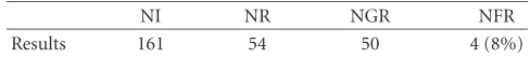
Table5: Result with a real mobile robot experimentation.
NI NR NGR NFR
Results 161 54 50 4 (8%)
5.3. Mobile robot localization
This experimentation has been done with a real mobile robot in our laboratory. There are also four places in this process but they are different from the previous experimentation. Yet, features are identical. The strategy here is different: dur-ing the learndur-ing phase and the generalization phase, the robot moves alone with its own speed, and images are issued from a continuous flow of images (“continuous” here means that the robot do not jump from one place to another, there are some ambiguous transition zones, difficult to classify).
The robot moves thus over the structured environment; 295 analyzed images give a 295×66 lookup table, the lattice of which is built with 8020 concepts. A total of 649 landmark concepts are extracted and 48 of them are isolated to be max-imal partial landmarks (17 from the place #1, 16 from the place #2, 9 from the place #3, and 6 from the place #4).
During the generalization phase (Table 5), the robot moves also over the same environment. 161 images are an-alyzed, 50 are well located in their respective place, and 4 are not. The global error is thus 8%, and the response rate is 33.5%. The reason of such alowresponse rate is that the robot moves through a white corridor that has very few fea-tures and landmarks, and a lot of white imagespollute the analysis rate. However, the number of (well or not) located images has no impact on our application: either the robot may give an answer (the place where it is) with a heuristic based on all image responses of the considered set (passive vision process), or the robot may look by itself for landmarks by moving around (active vision process). This is one of our next working orientations.
5.4. Experimentation with a bigger context
process, the lattice update time process depends on the im-age itself and the extracted features), and after 1100 imim-ages, the update process is longer if new images appear. In a place already visited, new combinations of features become scarce, so the update time process decreases. However, in a bigger environment, other techniques have to be implemented. A possible way to reduce the processing time is to split the en-vironment representation into local lattices. For instance, a lattice may cover a place and its topological neighbors. We are currently investigating this approach.
6. CONCLUSION AND PERSPECTIVES
In this paper, a new original supervised classification me-thod has been developed to classify images with respect to the place they have been taken. This method is strongly based on visual landmarks, anyone oranythingneeds to locate oneself. Our algorithms have been validated first through real im-ages issued from four different places of a structural envi-ronment, second through a comparison with an optimized neural network that gives lower-quality results with a lot of instability, and finally through a real experimentation with an autonomous mobile robot.
In this last case, a lot of heuristics could be developed to improve results, especially in introducing local constrains such as connected—or not—places, probabilities of transi-tion, and so forth. However, our objective here was to vali-date our algorithms in the worst case, that is, in a pure clas-sification problem without anya prioriknowledge.
Our system is open, that is, other attributes from any cap-tor could be used, or high-level attributes depending on the final purpose (e.g., “rectangles” for building in outside urban scenes). Thus we may incorporate “partially predefined land-mark” in the sense ofSection 2.1. Such an approach will be probably needed to process more complex tasks such as out-door localization in partially unknown environment. How-ever, in our applicative context, it was not necessary and this is worth to be noted.
Four main directions will lead our further research pro-gram. First, we have to improve our primitives and features in order to obtain a more stable and wider range of land-marks for the different classes. Second, we have to find a way to associate a symbolic classifier such as the concept lattice classifier we developed herein and a numerical classifier such as neural network to improve results. Indeed, results from these two techniques seem to be complementary, and prob-ably Galois lattices could preprocess a neural network clas-sifier through preselecting features. Afterwards, it would be valuable to introduce recent classification techniques such as “support vector machines.” Classification failures occur often on topological boundaries of the sites. Support vector tech-niques are supposed to help getting a more robust classifica-tion. Notice that the concept of margin is closer in its spirit from our “no decide” symbolic classifier. It is also important to investigate unsupervised classification methodologies to induce the creation of new classes, that is, nodes of the topo-logical map.
Support vector techniques are supposed to help getting a more robust classification and/or to induce the creation of new classes, that is, nodes of the topological map. Finally, in a more applicative way, our goal is to allow a robot to build a topological map of structured—or not—environment, in a fully autonomous process.
REFERENCES
[1] M. Knapek, R. S. Oropeza, and D. J. Kriegman, “Selecting promising landmarks,” inProc. IEEE International Conference on Robotics and Automation (ICRA ’00), vol. 4, pp. 3771–3777, San Francisco, Calif , USA, April 2000.
[2] G. Bianco and A. Zelinsky, “Biologically-inspired visual land-mark learning and navigation for mobile robots,” in Proc. IEEE/RSJ International Conference on Intelligent Robots and Systems (IROS ’99), vol. 2, pp. 671–676, Kyongju, South Ko-rea, October 1999.
[3] Z. Dodds and G. D. Hager, “A color interest operator for landmark-based navigation,” inProc. 14th National Confer-ence on Artificial IntelligConfer-ence and 9th Innovative Applications of Artificial Intelligence Conference (AAAI/IAAI ’97), pp. 655– 660, Providence, RI, USA, July 1997.
[4] G. Dudek and D. Jugessur, “Robust place recognition using local appearance based methods,” inProc. IEEE International Conference on Robotics and Automation (ICRA ’00), vol. 2, pp. 1030–1035, San Francisco, Calif , USA, April 2000.
[5] I. Ulrich and I. Nourbakhsh, “Appearance-based place recog-nition for topological localization,” inProc. IEEE International Conference on Robotics and Automation (ICRA ’00), vol. 2, pp. 1023–1029, San Francisco, Calif , USA, April 2000.
[6] R. Sim and G. Dudek, “Learning and evaluating visual fea-tures for pose estimation,” in Proc. 7th IEEE International Conference on Computer Vision (ICCV ’99), vol. 2, pp. 1217– 1222, Kerkyra, Greece, September 1999.
[7] M. Mata, J. M. Armingol, A. de la Escalera, and M. A. Salichs, “A visual landmark recognition system for topological naviga-tion of mobile robots,” inProc. IEEE International Conference on Robotics and Automation (ICRA ’01), vol. 2, pp. 1124–1129, Seoul, Korea, May 2001.
[8] S. Thompson, T. Matsui, and A. Zelinsky, “Localisation using automatically selected landmarks from panoramic images,” in Proc. Australian Conference on Robotics and Automation (ACRA ’00), Melbourne, Australia, August 2000.
[9] D. G. Lowe, “Object recognition from local scale-invariant features,” inProc. 7th IEEE International Conference on Com-puter Vision (ICCV ’99), vol. 2, pp. 1150–1157, Kerkyra, Greece, September 1999.
[10] J. B. Hayet, F. Lerasle, and M. Devy, “A visual landmark frame-work for indoor mobile robot navigation,” inProc. IEEE Inter-national Conference on Robotics and Automation (ICRA ’02), vol. 4, pp. 3942–3947, Washington, DC, USA, May 2002. [11] C. G. Harris and M. Stephens, “A combined corner and edge
detector,” inProc. 4th Alvey Vision Conference, pp. 147–151, Manchester, UK, August–December 1988.
[12] L. Itti, C. Koch, and E. Niebur, “A model of saliency-based visual attention for rapid scene analysis,”IEEE Trans. Pattern Anal. Machine Intell., vol. 20, no. 11, pp. 1254–1259, 1998. [13] A. Arleo, F. Smeraldi, S. Hug, and W. Gerstner, “Place cells and
spatial navigation based on 2D visual feature extraction, path integration, and reinforcement learning,” inAdvances in Neu-ral Information Processing Systems 13, pp. 89–95, MIT Press, Cambridge, Mass, USA, 2001.
cross fertilization,”Robotics and Autonomous Systems, vol. 30, no. 1-2, pp. 155–180, 2000.
[15] C. Schmid, R. Mohr, and C. Bauckhage, “Comparing and evaluating interest points,” inProc. 6th International Confer-ence on Computer Vision (ICCV ’98), pp. 230–235, Bombay, India, January 1998.
[16] S. O. Kuznetsov and S. A. Obiedkov, “Algorithms for the con-struction of concept lattices and their diagram graphs,” in Proc. 5th European Conference on Principles of Data Mining and Knowledge Discovery (PKDD ’01), vol. 2168, pp. 289–300, Freiburg, Germany, September 2001.
[17] R. Godin, R. Missaoui, and H. Alaoui, “Incremental con-cept formation algorithms based on Galois (concon-cept) lattices,” Computational Intelligence, vol. 11, no. 2, pp. 246–267, 1995. [18] M. Liqui`ere and J. Sallantin, “Structural machine learning
with Galois lattice and graphs,” in Proc. 15th International Conference on Machine Learning (ICML ’98), pp. 305–313, Madison, Wis, USA, July 1998.
[19] L. Chaudron, N. Maille, and M. Boyer, “The cube lattice model and its applications,” Applied Artificial Intelligence, vol. 17, no. 3, pp. 207–242, 2003.
[20] M. Barbut and B. Monjardet,Ordre et Classification, Hachette Universit´e, Paris, France, 1970.
[21] B. Ganter and R. Wille,Formal Concept Analysis: Mathemati-cal Foundations, Springer-Verlag, New York, NY, USA, 1999. [22] M. Boyer,Induction de r´egularit´es dans une base de
connais-sance, application au ph´enom`ene bruit/Gˆene et ses extensions, Ph.D. thesis, ´Ecole Nationale Sup´erieure de l’A´eronautique et de l’Espace, Toulouse, Cedex, France, 2001.
[23] S. O. Kuznetsov and S. A. Obiedkov, “Comparing perfor-mance of algorithms for generating concept lattices,”Journal of Experimental & Theoretical Artificial Intelligence, vol. 14, no. 2-3, pp. 189–216, 2002.
[24] E. M. Norris, “An algorithm for computing the maxi-mal rectangles in a binary relation,” Revue Roumaine de Math´ematiques Pures et Appliqu´ees, vol. 23, no. 2, pp. 243–250, 1978.
[25] P. Ranganathan, J. B. Hayet, M. Devy, S. Hutchinson, and F. Larasle, “Topological navigation and qualitative localization for indoor environments using multisensory perception,” in Proc. 9th International Symposium on Intelligent Robotic Sys-tems (SIRS ’01), Toulouse, Cedex, France, July 2001.
Emmanuel Zenouis a Research Engineer in ´Ecole Nationale Sup´erieure de l’A´eronau-tique et de l’Espace (SUPAERO), in col-laboration with the LAAS-CNRS, Toulouse, France. He recieved a Ph.D. in computer vision and computer science in 2004 from SUPAERO. His research deals with artificial intelligence, especially hierarchical struc-tures called Galois lattices, applied to com-puter vision and topological localization
and mapping. He is a graduate from ´Ecole Normale Sup´erieure, Cachan, and University of Paris XI, Orsay. He is also working as a Research Engineer in SUPAERO, in the fields of computer vi-sion, image processing, and machine learning. He manages many projects with postgraduate students in computer vision and control theory, applied to autonomous mobile robotics and drones. He col-laborates also with DGA (D´el´egation G´en´erale pour l’Armement) for image-based drone position control algorithms.
Manuel Samuelidesgraduated with an M.S. degree from ´Ecole Normale Sup´erieure, Paris, and Pierre et Marie Curie University (Paris VI) in 1969, and received a Ph.D. de-gree in mathematics from Paris VI Univer-sity in 1972. Since 1978, he has been ap-pointed as a Full Professor at ´Ecole Na-tionale Sup´erieure de l’A´eronautique et de l’Espace where he is in charge of the Depart-ment of Applied Mathematics and of the