R E S E A R C H
Open Access
Research on range-free location algorithm
for wireless sensor network based on
particle swarm optimization
Dalong Xue
Abstract
Location technology is the key support technology of wireless sensor network (WSN). The hop number and hop distance information obtained by traditional distance vector hop (DV-Hop) location algorithm can only be acquired by solving the nonlinear equations, and the solution of the equation determines the accuracy of node location. Although the least squares method has better estimation performance, the solution results are sensitive to the average hop distance, which will lead to the large error in the solution of the equation. In order to solve the problem of location error caused by initial value sensitivity of least squares method in the coordinate calculation stage of unknown nodes and beacon nodes, a range-free location algorithm based on particle swarm optimization (PSO) is proposed in this paper. The proposed approach solves the problem of location error caused by initial value sensitivity of least squares method, obtains relatively accurate solution, and improves the accuracy of location algorithm. The experimental results show that the PSO algorithm has faster convergence speed and higher location accuracy than the non-optimization algorithm.
Keywords:Wireless sensor network, Particle swarm optimization, DV-Hop algorithm, Least squares method
1 Introduction
Node location is a key technology in wireless sensor net-work, and its location accuracy is directly related to the overall performance of wireless sensor network (WSN) system [1, 2]. At present, the researches of WSN loca-tion algorithm have achieved rich results, and many novel solutions and ideas are used to solve the localization problem [3,4]. Among them, distance vector hop (DV-Hop) location algorithm is the most widely used method. This method has the advantages of low complexity and good scalability, but its location accuracy is lower [5]. In the traditional DV-Hop algorithm, the minimum hops between beacon nodes and unknown nodes and the average hop distance between beacon nodes are the main reasons for location errors. At the same time, the hop number and hop distance informa-tion obtained in the calculainforma-tion process of locainforma-tion algo-rithm usually use the least square method to solve the nonlinear equations in order to obtain the coordinates
of unknown nodes. Although the least squares method has better estimation performance, the final solution of the equation will have a large deviation due to its sensi-tivity to the initial value [6]. To solve the above prob-lems, many scholars optimized the nonlinear equations by using some optimization algorithms, such as anneal-ing algorithm, ant colony algorithm, and so on [7]. Through the iterative correction ability of these optimization algorithms, the error caused by the sensi-tivityto initial values is reduced.
In recent years, particle swarm optimization (PSO), as a bio-evolutionary algorithm, has attracted much attention and played an important role in solving optimization problems. Compared with other genetic algorithms, PSO algorithm has no crossover and muta-tion operamuta-tions, and it has fast search speed, high preci-sion, good memory, and easy to be implemented in engineering. Many scholars have introduced PSO algo-rithm into DV-Hop algoalgo-rithm. Because of its low sensi-tivity to measurement errors, PSO can achieve rapid optimization, thus the node location error is reduced [8]. In ref. [9], PSO is used to improve DV-Hop algorithm.
© The Author(s). 2019Open AccessThis article is distributed under the terms of the Creative Commons Attribution 4.0 International License (http://creativecommons.org/licenses/by/4.0/), which permits unrestricted use, distribution, and reproduction in any medium, provided you give appropriate credit to the original author(s) and the source, provide a link to the Creative Commons license, and indicate if changes were made.
Correspondence:[email protected]
The simulation results show that the location accuracy and location coverage are better than traditional DV-Hop location algorithm, but PSO algorithm is easy to fall into local optimum. In ref. [10], PSO is firstly introduced into the localization problem of wireless sensor network based on range-free method. Compared with the existing centroid localization method, it greatly improves the localization accuracy. However, when the nodes are dis-tributed dispersedly in the network, the algorithm will cause large location errors. Reference [11] can use PSO to find the optimal location of the target node, but it in-creases the complexity of calculation, and affects the lo-cation effect of the node to some extent. Reference [12] proposes to optimize DV-Hop localization algorithm by using the connectivity difference between nodes. More-over, the experimental results show that the algorithm has higher localization accuracy than traditional DV-Hop algorithm.
In order to solve the problem of location error caused by initial value sensitivity of least squares method in the coordinate calculation stage of unknown nodes and bea-con nodes, a range-free location algorithm based on PSO is proposed in this paper. The proposed approach can solve the problem of location error caused by initial value sensitivity of least squares method, obtain rela-tively accurate solution, and improve the accuracy of location algorithm.
2 Description on location problem
Figure 1 shows the distribution of unknown nodes and beacon nodes. When the unknown node obtains more than three distances from the beacon nodes, the posi-tioning accuracy can be improved by using the redun-dant distance information. At this time, the least square method can be used to estimate the position of the unknown node.
The location process of DV-Hop algorithm can be divided into three stages. In the first and second stages, the estimated distances from unknown node O(x,y) to beacon nodes A1(x1,y1),A2(x2,y2),A3(x3,y3), After expansion, the following equations can be obtained:
more accurate the estimation position is, and the smaller the value of f(x,y) in Eq. (2) is. Therefore, the location problem can be transformed into solving the minimum value problem of nonlinear equations, that is, solving the estimated coordinate (x,y) to minimize the value of f(x,y) in Eq. (2). Fitness function is used to evalu-ate the quality of particle position and guide the search direction of the algorithm. Fitness function is defined as:
the distance from unknown node to beacon nodei.
3 The classical PSO algorithm
3.1 The basic principle of PSO algorithm
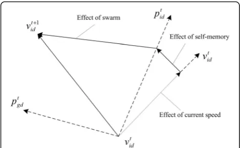
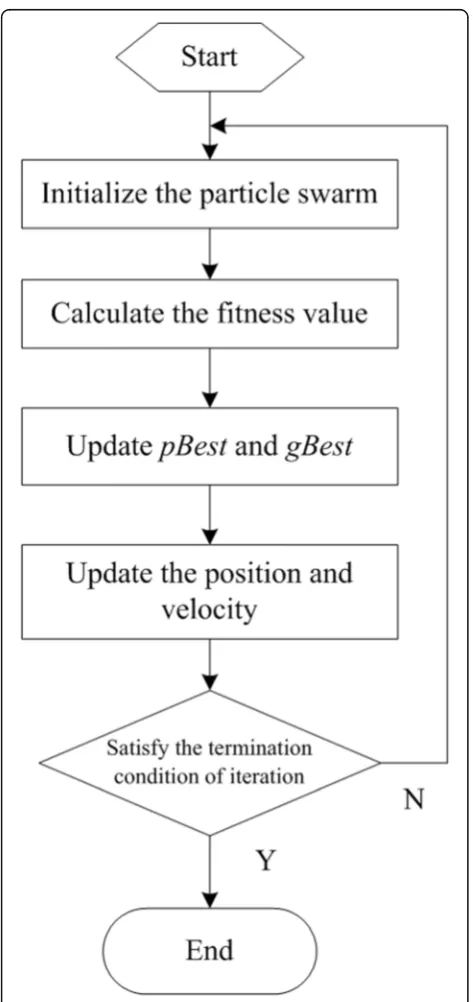
In the optimization process of PSO algorithm, every possible optimal position is usually treated as a particle, and each particle has a related fitness function to control the motion benchmark of particle in the optimization process of algorithm. At the same time, in the process of particle moving to the optimal“food,”there is also a vec-tor velocity to control the moving direction and speed of the particle in optimization region. Each particle can up-date its position in the optimal solution space by iter-ation optimiziter-ation model, and the updating method of particle position is shown in Fig.2.
In Fig.2,xis the initial position of the particle,vis the “flying”velocity of the particle, andpis the optimal pos-ition of the particle to be searched. In the process of searching for the optimal particle position iteratively, each particle updates and moves its position by record-ing and updatrecord-ing two key values which are closely re-lated to its position in the current optimization space. The two key values are the best individual position and the best global position of particle.
swarm is a D-dimensional space, then each particle in the particle swarm can be represented as the position vector, which is shown in Eq. (3):
Xi¼ðxi1;xi2;Λ;xiDÞ; i¼1;2;Λ;N ð3Þ
The velocity vector of each particle can be recorded as:
Vi¼ðvi1;vi2;Λ;xiDÞ; i¼1;2;Λ;N ð4Þ
The best individual location that each particle has ex-perienced can be recorded as:
Pbest ið Þ¼ðpi1;pi2;Λ;piDÞ; i¼1;2;Λ;N ð5Þ
From the beginning iteration to the current iteration of particle, the best position for all particles can be re-corded as follows:
gbest¼pg1;pg2;Λ;pgD ð6Þ
After obtaining the best individual position and the best global position of each particle, the velocity and position of each particle in the iterative optimization process can be updated according to the following two equations:
vtidþ1¼ωvtidþc1r1 ptid−xtid
þc2r2 ptgd−xtid
ð7Þ
xtidþ1¼xtidþvtid ð8Þ
Where ω is the inertia weight of the particles, c1and
c2 are learning factors, also known as acceleration
con-stants, and r1 and r2 are uniform random numbers in
the range of [0,1].
3.2 Analysis on algorithm parameters
According to Eqs. (7) and (8), there are four key parame-ters in PSO algorithm: inertia weight ω, learning factors c1andc2, which can control the velocity change during
iteration process of particle, and then control the
trajectory of particle in the whole optimization process. The maximum velocity vmax represents the position
moving step of the particle in unit time, and it reflects the speed of searching for the optimal solution of the particle. Therefore, they have great influence on the whole PSO algorithm.
1. Inertia weightω
The inertia weight coefficient weights the last iteration speed of the current particle, which can increase the searching ability of the particle toward the optimal solu-tion in the current iterasolu-tion process. Increasing the value of inertia weight can keep the particle moving toward the far potential optimal position. Meanwhile, reducing the value of inertia weight can weaken the searching ability of the particle in the optimization space, and it can only search the optimal value locally in the current region near the particle. When the inertia weight value is zero, the velocity updating of the particle in the current iteration process only depends on the best pos-ition that the individual has experienced and the global best position that all the particles have experienced, and it does not need to refer to the velocity value of the last particle, which results in the deviation of the particle in the process of searching for the optimal solution. There-fore, when the actual algorithm is solved iteratively, the value of the inertia weight needs to be adjusted, so as to control the particles to approach the optimal solution quickly, and to balance the iteration efficiency and optimization accuracy of the algorithm.
2. Learning factorsc1andc2
The learning factorsc1andc2can control the effect of
the best position experienced by each individual and the best position experienced by all particles on the velocity updating. Moreover, the particles can control the opti-mal path by referring to these two values. Without the existence ofc1andc2, the particle will fly straight at the
initial speed until it reaches the boundary area of the op-timal solution space, and the possibility of searching the optimal value is greatly reduced. In order to get the best solution of PSO in the process of optimization, the learning factorsc1and c2should also change with the
it-eration condition of particle swarm.
3. Maximum velocity of particlevmax
During the iteration process, the maximum velocity vmaxrepresents the position moving step of the particle
of the particle in each dimension is always set asvdmax=
k×xdmax, 0.1≤k≤1, where xdmax represents the length
of each dimension of the optimization space.
3.3 The process of PSO algorithm
The concrete process of particle swarm optimization is shown in Fig.3.
The specific steps of particle swarm optimization are as follows:
Step 1: Assuming that the number of particles in the population isn, and thesenparticles are generated ran-domly. The velocityviand positionxiof the particles are
assigned the initial values, and the individual optimal so-lution is the current position of the particles.
Step 2: According to Eq. (9), the fitness function values of all particles are obtained.
F xð ;yÞ ¼
ffiffiffiffiffiffiffiffiffiffiffiffiffiffiffiffiffiffiffiffiffiffiffiffiffiffiffiffiffiffiffiffiffiffi
x−xi
ð Þ2þ
y−yi ð Þ2 q
−di ð9Þ
Step 3: According to Eqs. (10) and (11), the individual and global optimal values of particles are updated.
pBesttþ1¼ x
tþ1; if F X tþ1≤F pBestð tÞ
pBesttþ1; if F X tþ1> F pBestð tÞ
ð10Þ
gBesttþ1¼ pBest
tþ1; if F pBest tþ1≤F gBestð tÞ
gBestt; if F pBest tþ1> F gBestð tÞ
ð11Þ
Step 4: The velocity and position of particles are up-dated according to Eqs. (7) and (8).
Step 5: Finding the fitness function that meets the conditions or the number of iterations will terminate the algorithm. Otherwise, continue step 2 to find the opti-mal particle.
Step 6: The particle corresponding to the global opti-mal value is obtained as the estimated position of the unknown node.
4 The improved PSO algorithm
4.1 The improvement on algorithm
In the standard POS algorithm, the learning factors c1 and c2 are generally set as two fixed parameters, which have a great impact on the algorithm. In differ-ent periods of population evolution, the search per-formance of particles is different. Generally speaking, in the global search scenario, the algorithm should have better search performance for the initial stage; in the end stage of the algorithm, the algorithm should have better development ability to improve the convergence speed of the algorithm. If a fixed acceler-ation coefficient is used in the algorithm, it will inev-itably limit the ability of particles to adjust the search step and flight direction in flight period. Therefore, in this paper, two acceleration factors are added to the traditional POS algorithm, which can adapt to change.
Ai1¼ ln
f Pð ið Þt Þ−f Xð ið Þt Þ
PF
þe−1
ð12Þ
Ai2¼ ln lation, f(x) is the objective function, e is the base of natural logarithm, and PF represents the mean of the difference between the individual fitness and the opti-mal value of a single particle in a population. There-fore, if jfðPiðtÞÞ−fðXiðtÞÞ>jPFjj exists, there will be Ai1> 1, which means the particle will be accelerated.
Meanwhile, if jfðPiðtÞÞ−fðXiðtÞÞ<jPFjj exists, there will be Ai1< 1, which means the particle will be
decel-erated. Similarly, GF represents the mean value of the difference between individual fitness and population optimal values of all particles in a population. There-fore, if jfðPgðtÞÞ−fðXiðtÞÞ>jGFjj exists, there will be Ai2> 1, which means the particle will be accelerated.
Meanwhile, if jfðPgðtÞÞ−fðXiðtÞÞ<jGFjj exists, there will be Ai2< 1, which means the particle will be
decelerated.
The cognitive and social coefficients used in this paper are shown as follows:
ω1¼
Where c1and c2are the same as the acceleration
con-stants of traditional PSO algorithm.
In the traditional PSO algorithm, ω(t) decreases linearly along with the increase of the number of evolutions.
ωð Þ ¼t ðωi−ωcÞðTmax−tÞ
Tmax þωc ð
16Þ
Where t is the current iteration number, ωi is the
initial inertia weight, Tmax is the largest iteration
number, ωc is the inertia weight when iterating to the
algebraic maximum, and ωmax = 0.9 and ωmin = 0.4.
With the increase of iteration, ω(t) will gradually de-crease, which makes the algorithm have stronger glo-bal search performance in the initial stage and increases the possibility of obtaining global optimal solution. At the end of the algorithm, the smaller weight can give the particle stronger local search per-formance and improve the convergence speed of the algorithm.
The influence of inertia weight ω on PSO algorithm is shown as follows: when the value of ω is too large, it can prevent the algorithm from entering the local
optimal result. Meanwhile, when the value of ω is too small, it can make the algorithm search locally more effectively and improve the convergence speed of the algorithm.
According to the above analysis, this paper proposes that the inertia weight is a random, linear, and decreas-ing weight in the later iteration stage, so that the ω of particle will get a larger value in the initial stage of the algorithm in order to guarantee the diversity of the par-ticle. Meanwhile, at the end of the algorithm, the ω of particle are likely to get larger, so as to get out of the local extremum. The value of random inertia weight ω varies with the number of iterations:
ω¼ωmax−ðωmax−ωminÞ
t
Tmax ð
17Þ
When the number of iterations is larger than 0.7Tmax,
there is ω= 0.4 + 0.3∗ rand(). The function rand( ) is used to generate a random number that is evenly distrib-uted between 0 and 1.
Then the equation of inertia weight ω for the whole process of the algorithm is shown as follows:
ωð Þ ¼t ωmax−ðωmax−ωminÞ
Therefore, the evolution equation of the adaptive PSO algorithm is shown as follows:
vkidþ1¼ωð Þ t vkidþω1 randðÞAi1 pid−xkid
4.2 Selection of fitness function
When estimating the distance between unknown node and beacon nodes in DV-Hop algorithm, the average hop distance and the hops of beacon nodes between two nodes are mainly used to calculate it, which has certain errors. Assuming that the beacon nodes are P1(x1,y1), P1(x2,y2), ..., P1(xn,yn), the
esti-mated distances between unknown node and each beacon node obtained by step 1 and step 2 of DV-Hop algorithm are respectively d1, d2, d3,...,dn, and
the differences between estimated distance and real distance are respectively ε1, ε2, ε3, ..., εn. From the
ffiffiffiffiffiffiffiffiffiffiffiffiffiffiffiffiffiffiffiffiffiffiffiffiffiffiffiffiffiffiffiffiffiffiffiffi
The coordinate ð^x;^yÞ of unknown node should satisfy all the equations mentioned above. When the sum of |ε1|,|ε2|,..., and |εn| is smaller, the accuracy of estimating
coordinate ð^x;^yÞ is higher. Therefore, to some extent, the optimization of PSO algorithm for estimating coord-inate of unknown node can be transformed into the process of minimizing Eq. (22).
fið^x;^yÞ ¼
PSO algorithm uses the current particle fitness value to distinguish the advantages and disadvantages of its specific location in the optimization stage. In the current population, any particle is the coordinate possible solution of the unknown node. This paper mainly distinguishes the advantages and disadvantages of any particle through the current fitness function expressed by Eq. (23):
Where ndenotes the number of beacon nodes, andhi
denotes the number of hops from unknown nodes to beacon nodes. In order to avoid excessive hops between unknown nodes and beacon nodes, which results in af-fecting estimation distance too much from cumulative errors, hi is added into the fitness function in order to
reduce the impact of excessive hops. In contrast, when hi becomes larger, the influence of the beacon node on
the accuracy of fitness becomes smaller.
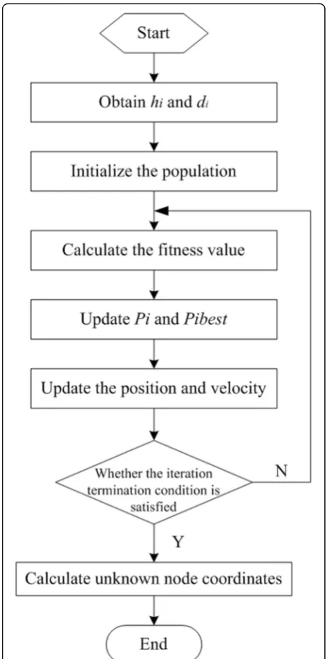
The localization process of the improved algorithm is shown in Fig.4.
5 Experimental results and analysis
In order to verify the location effect of PSO optimization al-gorithm, the traditional DV-Hop location algorithm and the improved PSO-based DV-Hop algorithm are simulated on the Matlab experimental platform. In the same network environment, the performance of the algorithm is com-pared by changing beacon nodes, communication radius.
The simulation environment is shown as follows: (1) all sensor nodes are arbitrarily arranged in the network environment; (2) the number of unknown nodes is 200, and the communication radius of nodes is 15 m; (3) the number of beacon nodes is 30, and they are arbitrarily distributed in the monitoring area, and each broadcast radiation distance can reach the whole network. In the
network, the population size is 20 and the maximum number of evolutionary iterations of particles in the par-ticle swarm is 300. According to Eq. (18), the inertia weight ω is changed fromωmax= 0.9 toωmin= 0.4, and
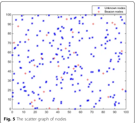
the learning factors are chosen as c1= c2= 2. Figure 5
shows the scatter graph of nodes.
5.1 Influences of beacon node density on algorithm Each group of data is the result after 60 times average. In the network topology shown in Fig.4, the communication
radiusR= 15 m is simulated when proportion of beacon nodes from 5 to 30% of the total number of nodes. The experimental results are shown in Fig.6.
Under the condition of the same beacon node dens-ity, the error rate of the improved PSO DV-Hop algo-rithm is not greater than that of the traditional DV-Hop algorithm. When the proportion of beacon nodes is 10–25%, the momentum of improving the location accuracy is obvious for PSO optimization algorithm; when the density of beacon nodes exceeds 25%, the lo-cation accuracy of the algorithm increases slowly. Moreover, the increasing trend of traditional DV-Hop algorithm is also slowing down, which shows that when the number of beacon nodes in the environment is large, the location accuracy of the algorithm tends to
be stable. When the density of beacon nodes is the same, the location accuracy of the improved algorithm is better than that of the traditional DV-Hop algorithm in the network environment.
5.2 Influences of communication radius on algorithm In the same experiment simulation, we mainly depend on changing the communication radius of unknown nodes to investigate the influence of network connectiv-ity on the algorithm. The total number of nodes scat-tered in the environment is 200, the sparse density of beacon nodes is adjusted to 20%, and the transformation range of communication radius is [15 m, 40 m]. The simulation results are shown in Fig.7.
Figure 7 shows that the improved PSO algorithm outperforms the traditional DV-Hop algorithm in loca-tion accuracy when the communicaloca-tion radius is small. In the process of changing the communication radius from 15 to 40 m, the location accuracy of the two algorithms shows an improving trend, and the attenu-ation degree of the locattenu-ation error of the improved al-gorithm is still better than that of the traditional DV-Hop algorithm.
6 Conclusion
In order to solve the problem of location error caused by initial value sensitivity of least squares method in the coordinate calculation stage of unknown nodes and bea-con nodes, a range-free location algorithm based on par-ticle swarm optimization (PSO) is proposed in this paper. The proposed approach solves the problem of lo-cation error caused by initial value sensitivity of least squares method, obtains relatively accurate solution, and improves the accuracy of location algorithm. In order to verify the location effect of PSO optimization algorithm, Fig. 5The scatter graph of nodes
the traditional DV-Hop location algorithm and the im-proved PSO-based DV-Hop algorithm are simulated on the Matlab experimental platform. In the same network environment, the performance of the algorithm is com-pared by changing beacon nodes, communication radius. The experimental results show that the PSO algorithm has faster convergence speed and higher location accur-acy than the non-optimization algorithm.
Abbreviation
WSN:Wireless sensor network; DV-Hop: Distance vector hop; PSO: Particle swarm optimization
Acknowledgements Not applicable.
Authors’contributions
The author completed the experiment and manuscript. The author read and approved the final manuscript.
Authors’information
Dalong Xue: PhD student, School of Computer Science and Technology, Beijing Institute of Technology. His research interests include computer network technology, software algorithm.
Funding Not applicable.
Availability of data and materials
The data generated and analyzed during this study are included in this published article, and its supplementary information is also available from the corresponding author on reasonable request.
Competing interests
The author declares that he has no competing interest.
Received: 19 June 2019 Accepted: 16 August 2019
References
1. F.L. Lewis, Wireless sensor networks[J]. Smart Environ. Technol. Protoc. Appl. 181(1), 11–46 (2016)
2. R. Shahbazian, S.A. Ghorashi, Distributed cooperative target detection and localization in decentralized wireless sensor networks[J]. J. Supercomput. 73(4), 1715–1732 (2017)
3. M. Zhang, D. Zhang, F. Goerlandt, X. Yan, P. Kujala, Use of HFACS and fault tree model for collision risk factors analysis of icebreaker assistance in ice-covered waters. Saf. Sci.111, 128–143 (2019)
4. J. Fernandez-Bes, J. Arenas-Garca, M.T.M. Silva, et al., L. A. Azpicueta-Ruiz, Adaptive diffusion schemes for heterogeneous networks[J]. IEEE Trans. Signal Process.65(21), 5661–5674 (2017)
5. N.A.M. Maung, M. Kawai, Experimental evaluations of RSS threshold-based optimised DV-HOP localisation for wireless ad-hoc networks [J]. Electron. Lett.50(17), 1246–1248 (2014)
6. G. Song, D. Tam, Two novel DV-Hop localization algorithms for randomly deployed wireless sensor networks[J]. Int. J. Distrib. Sens. Netw.9, 1–12 (2015)
7. M.R. Tanweer, R. Auditya, S. Suresh, Directionally driven self-regulating particle swarm optimization algorithm[J]. Swarm Evol. Comput.28, 98–116 (2016)
8. Y. Zhang, J. Liang, S. Jiang, et al., A localization method for underwater wireless sensor networks based on mobility prediction and particle swarm optimization algorithms[J]. Sensors16(2), 212.GB/T 7714 (2016)
9. Z. Fengrong, Positioning research for wireless sensor networks based on PSO algorithm[J]. Elektronika Ir Elektrotechnika19(9), 7–10 (2013) 10. H. Bao, B. Zhang, C. Li, et al., Mobile anchor assisted particle swarm
optimization (PSO) based localization algorithms for wireless sensor networks[J]. Wirel. Commun. Mob. Comput.12(15), 1313–1325 (2012)
11. H.A. Nguyen, H. Guo, K.S. Low, Real-time estimation of sensor node's position using particle swarm optimization with log-barrier constraint[J]. Instrum. Meas. IEEE Trans.60(11), 3619–3628 (2011)
12. L. Gui, T. Val, A. Wei, et al., Improvement of range-free localization technology by a novel DV-hop protocol in wireless sensor networks[J]. Ad Hoc Netw.24, 55–73 (2015)
Publisher’s Note