Type Based MCMC

Type-Based MCMC

Percy Liang UC Berkeley [email protected]

Michael I. Jordan UC Berkeley [email protected]

Dan Klein UC Berkeley [email protected]

Abstract

Most existing algorithms for learning latent-variable models—such as EM and existing Gibbs samplers—are token-based, meaning that they update the variables associated with one sentence at a time. The incremental na-ture of these methods makes them suscepti-ble to local optima/slow mixing. In this paper, we introduce atype-based sampler, which up-dates a block of variables, identified by atype, which spans multiple sentences. We show im-provements on part-of-speech induction, word segmentation, and learning tree-substitution grammars.

1 Introduction

A long-standing challenge in NLP is the unsu-pervised induction of linguistic structures, for ex-ample, grammars from raw sentences or lexicons from phoneme sequences. A fundamental property of these unsupervised learning problems is multi-modality. In grammar induction, for example, we could analyze subject-verb-object sequences as ei-ther ((subject verb) object) (mode 1) or (subject (verb object))(mode 2).

Multimodality causes problems for token-based procedures that update variables for one example at a time. In EM, for example, if the parameters al-ready assign high probability to the((subject verb) object)analysis, re-analyzing the sentences in E-step only reinforces the analysis, resulting in EM getting stuck in a local optimum. In (collapsed) Gibbs sam-pling, if all sentences are already analyzed as ((sub-ject verb) ob((sub-ject), sampling a sentenceconditioned

2 1 2 2 1

2 2 2 1 2

1 2 1 2 2

2 1 2 2 1

2 2 2 1 2

1 2 1 2 2

2 1 2 2 1

2 2 2 1 2

1 2 ₁ 2 2

(a) token-based (b) sentence-based (c) type-based

Figure 1: Consider a dataset of 3 sentences, each of length 5. Each variable is labeled with atype(1 or 2). The unshaded variables are the ones that are updated jointly by a sampler. The token-based sampler updates the vari-able for one token at a time (a). The sentence-based sam-pler updates all variables in a sentence, thus dealing with intra-sentential dependencies (b). The type-based sam-pler updates all variables of a particular type (1 in this ex-ample), thus dealing with dependencies due to common parameters (c).

on all others will most likely not change its analysis, resulting in slow mixing.

To combat the problems associated with token-based algorithms, we propose a new sampling algo-rithm that operates ontypes. Our sampler would, for example, be able to change all occurrences of ((sub-ject verb) ob((sub-ject) to (subject (verb object)) in one step. These type-based operations are reminiscent of the type-based grammar operations of early chunk-merge systems (Wolff, 1988; Stolcke and Omohun-dro, 1994), but we work within a sampling frame-work for increased robustness.

In NLP, perhaps the the most simple and popu-lar sampler is thetoken-based Gibbs sampler,1used in Goldwater et al. (2006), Goldwater and Griffiths (2007), and many others. By sampling only one

1_{In NLP, this is sometimes referred to as simply the}

col-lapsed Gibbs sampler.

variable at a time, this sampler is prone to slow mix-ing due to the strong couplmix-ing between variables. A general remedy is to sample blocks of coupled variables. For example, thesentence-based sampler samples all the variables associated with a sentence at once (e.g., the entire tag sequence). However, this blocking does not deal with the strong type-based coupling (e.g., all instances of a word should be tagged similarly). The type-based sampler we will present is designed exactly to tackle this coupling, which we argue is stronger and more important to deal with in unsupervised learning. Figure 1 depicts the updates made by each of the three samplers.

We tested our sampler on three models: a Bayesian HMM for part-of-speech induction (Gold-water and Griffiths, 2007), a nonparametric Bayesian model for word segmentation (Goldwater et al., 2006), and a nonparametric Bayesian model of tree substitution grammars (Cohn et al., 2009; Post and Gildea, 2009). Empirically, we find that type-based sampling improves performance and is less sensitive to initialization (Section 5).

2 Basic Idea via a Motivating Example

The key technical problem we solve in this paper is finding a block of variables which are both highly coupled and yet tractable to sample jointly. This section illustrates the main idea behind type-based sampling on a small word segmentation example.

Suppose our datasetx consists ofnoccurrences of the sequence a b. Our goal is infer z = (z1, . . . , zn), where zi = 0 if the sequence is one

word ab, and zi = 1 if the sequence is two, a

and b. We can model this situation with a simple generative model: for each i = 1, . . . , n, gener-ate one or two words with equal probability. Each word is drawn independently based on probabilities θ = (θa, θb, θab) which we endow with a uniform

priorθ∼Dirichlet(1,1,1).

We marginalize outθto get the following standard expression (Goldwater et al., 2009):

p(z|x)∝ 1

(m)₁(m)₁(n−m)

3(n+m)

def

= g(m), (1)

wherem =Pn

i=1zi is the number of two-word

se-quences anda(k) =a(a+ 1)· · ·(a+k−1)is the

200 400 600 8001000 m -1411.4

-1060.3 -709.1 -358.0 -6.8

log

g

(

m

)

2 4 6 8 10

iteration

200 400 600 800 1000

m

Token Type

(a) bimodal posterior (b) sampling run

Figure 2: (a) The posterior (1) is sharply bimodal (note the log-scale). (b) A run of the token-based and type-based samplers. We initialize both samplers withm=n (n = 1000). The type-based sampler mixes instantly (in fact, it makes independent draws from the posterior) whereas the token-based sampler requires five passes through the data before finding the high probability re-gionm_u0.

ascending factorial.2 Figure 2(a) depicts the result-ing bimodal posterior.

A token-based sampler chooses onezi to update

according to the posteriorp(zi | z−i,x). To

illus-trate the mixing problem, consider the case where m = n, i.e., all sequences are analyzed as two words. From (1), we can verify that p(zi = 0 |

z−i,x) = O(_n1). Whenn = 1000, this means that

there is only a 0.002 probability of setting zi = 0,

a very unlikely but necessary first step to take to es-cape this local optimum. Indeed, Figure 2(b) shows how the token-based sampler requires five passes over the data to finally escape.

Type-based sampling completely eradicates the local optimum problem in this example. Let us take a closer look at (1). Note thatp(z|x)only depends on a single integerm, which only takes one ofn+ 1 values, not on the particularz. This shows that the zis are exchangeable. There are _mn

possible val-ues ofzsatisfyingm = P

izi, each withthe same

probabilityg(m). Summing, we get:

p(m|x)∝ X

z:m=P izi

p(x,z) =

n m

g(m). (2)

A sampling strategy falls out naturally: First, sample the numberm via (2). Conditioned on m, choose

2

the particularz uniformly out of the _mn

possibili-ties. Figure 2(b) shows the effectiveness of this type-based sampler.

This simple example exposes the fundamental challenge of multimodality in unsupervised learn-ing. Bothm = 0andm =nare modes due to the rich-gets-richer property which arises by virtue of allnexamples sharing the same parametersθ. This sharing is a double-edged sword: It provides us with clustering structure but also makes inference hard. Even thoughm=nis much worse (by a factor ex-ponential inn) thanm = 0, a na¨ıve algorithm can easily have trouble escapingm=n.

3 Setup

We will now present the type-based sampler in full generality. Our sampler is applicable to any model which is built out of local multinomial choices, where each multinomial has a Dirichlet process prior (a Dirichlet prior if the number of choices is finite). This includes most probabilistic models in NLP (ex-cluding ones built from log-linear features).

As we develop the sampler, we will pro-vide concrete examples for the Bayesian hidden Markov model (HMM), the Dirichlet process uni-gram segmentation model (USM) (Goldwater et al., 2006), and the probabilistic tree-substitution gram-mar (PTSG) (Cohn et al., 2009; Post and Gildea, 2009).

3.1 Model parameters

A model is specified by a collection of multino-mial parameters θ = {θr}r∈R, where R is an in-dex set. Each vectorθr specifies a distribution over

outcomes: outcomeohas probabilityθro.

• HMM: Let K is the number of states. The set

R = {(q, k) : q ∈ {T,E}, k = 1, . . . , K}

indexes the K transition distributions {θ_(T,k)}

(each over outcomes {1, . . . , K}) and K emis-sion distributions {θ(E,k)} (each over the set of

words).

• USM:R={0}, andθ0is a distribution over (an

infinite number of) words.

• PTSG: R is the set of grammar symbols, and each θr is a distribution over labeled tree

frag-ments with root labelr.

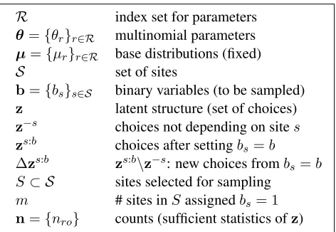
R index set for parameters θ={θr}r∈R multinomial parameters µ={µr}r∈R base distributions (fixed) S set of sites

b={bs}s∈S binary variables (to be sampled) z latent structure (set of choices) z−s choices not depending on sites

zs:b _{choices after settingb} s=b

∆zs:b zs:b\z−s_{: new choices fromb} s=b S⊂ S sites selected for sampling

m # sites inSassignedbs= 1

n={nro} counts (sufficient statistics ofz)

Table 1: Notation used in this paper. Note that there is a one-to-one mapping betweenzand(b,x). The informa-tion relevant for evaluating the likelihood isn. We use the following parallel notation: n−s _{= n(z}−s_),ns:b ₌ n(zs:b_),∆ns_=n(∆zs_).

3.2 Choice representation of latent structurez

We represent the latent structurez as a set of local choices:3

• HMM: z contains elements of the form (T, i, a, b), denoting a transition from state a at position i to state b at position i+ 1; and (E, i, a, w), denoting an emission of word w from stateaat positioni.

• USM:zcontains elements of the form(i, w), de-noting the generation of wordwat character po-sitioniextending to positioni+|w| −1.

• PTSG:zcontains elements of the form(x, t), de-noting the generation of tree fragmenttrooted at nodex.

The choiceszare connected to the parametersθ

as follows: p(z | θ) = Q

z∈zθz.r,z.o. Each choice z ∈ z is identified with some z.r ∈ R and out-comez.o. Intuitively, choicezwas made by drawing drawingz.ofrom the multinomial distributionθz.r.

3.3 Prior

We place a Dirichlet process prior onθr (Dirichlet

prior for finite outcome spaces): θr ∼ DP(αr, µr),

where αr is a concentration parameter and µr is a

fixed base distribution.

3_{We assume thatzcontains both a latent part and the}

Letnro(z) =|{z∈z :z.r =r, z.o=o}|be the

number of draws fromθrresulting in outcomeo, and nr·=P_onrobe the number of timesθrwas drawn

from. Let n(z) = {nro(z)} denote the vector of

sufficient statistics associated with choicesz. When it is clear from context, we simply writenforn(z). Using these sufficient statistics, we can writep(z |

θ) =Q

r,oθ nro(z)

ro .

We now marginalize out θ using Dirichlet-multinomial conjugacy, producing the following ex-pression for the likelihood:

p(z) = Y

r∈R Q

o(αroµro)(nro(z)) αr(nr·(z))

, (3)

wherea(k)=a(a+1)· · ·(a+k−1)is the ascending factorial. (3) is the distribution that we will use for sampling.

4 Type-Based Sampling

Having described the setup of the model, we now turn to posterior inference ofp(z|x).

4.1 Binary Representation

We first define a new representation of the latent structure based on binary variablesbso that there is a bijection betweenzand(b,x);zwas used to de-fine the model,bwill be used for inference. We will useb to exploit the ideas from Section 2. Specifi-cally, letb={bs}s∈Sbe a collection of binary vari-ables indexed by a set ofsitesS.

• HMM: If the HMM hasK= 2states,Sis the set of positions in the sequence. For eachs∈ S,bs

is the hidden state ats. The extension to general Kis considered at the end of Section 4.4.

• USM: S is the set of non-final positions in the sequence. For eachs ∈ S, bs denotes whether

a word boundary exists between positionssand s+ 1.

• PTSG:S is the set of internal nodes in the parse tree. Fors ∈ S,bs denotes whether a tree

frag-ment is rooted at nodes.

For each sites ∈ S, letzs:0 andzs:1 denote the choices associated with the structures obtained by setting the binary variable bs = 0andbs = 1,

re-spectively. Define z−s def= zs:0∩zs:1 to be the set

of choices that do notdependon the value ofbs, and

n−sdef= n(z−s)be the corresponding counts.

• HMM: z−s includes all but the transitions into and out of the state atsplus the emission ats.

• USM:z−s_{includes all except the word ending at} sand the one starting ats+ 1if there is a bound-ary (bs = 1); except the word coverings if no

boundary exists (bs= 0).

• PTSG:z−s includes all except the tree fragment rooted at nodesand the one with leafsifbs= 1;

except the single fragment containingsifbs= 0.

4.2 Sampling One Site

A token-based sampler considers one sitesat a time. Specifically, we evaluate the likelihoods ofzs:0and zs:1according to (3) and samplebswith probability

proportional to the likelihoods. Intuitively, this can be accomplished by removing choices that depend onbs(resulting inz−s), evaluating the likelihood

re-sulting from settingbsto 0 or 1, and then adding the

appropriate choices back in.

More formally, let∆zs:b def= zs:b\z−s be the new choices that would be added if we set bs = b ∈ {0,1}, and let ∆ns:b def= n(∆zs:b) be the corre-sponding counts. With this notation, we can write the posterior as follows:

p(bs=b|b\bs)∝ (4)

Y

r∈R Q

o(αroµro+n −s ro)

(∆nsro:b)

(αr+n−r·s)(∆n

s:b r· )

.

The form of the conditional (4) follows from the joint (3) via two properties: additivity of counts (ns:b = n−s+ ∆ns:b) and a simple property of as-cending factorials (a(k+δ) =a(k)(a+k)(δ)).

In practice, most of the entries of∆ns:bare zero. For the HMM, ns:b

ro would be nonzero only for

the transitions into the new state (b) at position s (zs−1 →b), transitions out of that state (b→zs+1),

and emissions from that state (b→xs).

4.3 Sampling Multiple Sites

We would like to sample multiple sites jointly as in Section 2, but we cannot choose any arbitrary subset S ⊂ S, as the likelihood will in general depend on

the exact assignment ofbS def

a b c a a b c a b c b

(a) USM

1 1 2 2 1 1 2 2 a b a b c b b e

(b) HMM

a

b

a a

b c

d e

c

d

b c

e

a b

(c) PTSG

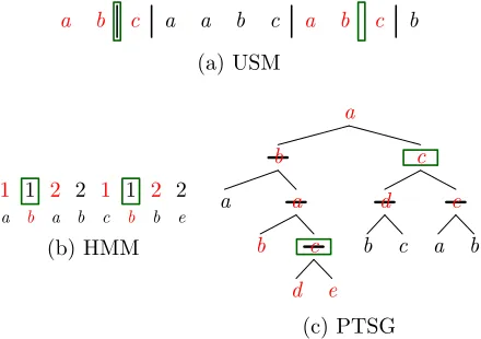
Figure 3: The type-based sampler jointly samples all vari-ables at a set of sitesS (in green boxes). Sites inS are chosen based on types (denoted in red). (a) HMM: two sites have the same type if they have the same previous and next states and emit the same word; they conflict un-less separated by at least one position. (b) USM: two sites have the same type if they are both of the formab|c or abc; note that occurrences of the same letters with other segmentations do not match the type. (c) PTSG: analo-gous to the USM, only for tree rather than sequences.

there are an exponential number. To exploit the ex-changeability property in Section 2, we need to find sites which look “the same” from the model’s point of view, that is, the likelihood only depends on bS

viamdef= P

s∈Sbs.

To do this, we need to define two notions,typeand conflict. We say sitessands0 have the sametypeif the counts added by setting either bs orbs0 are the

same, that is,∆ns:b = ∆ns0:b forb ∈ {0,1}. This motivates the following definition of thetypeof site swith respect toz:

t(z, s)def= (∆ns:0,∆ns:1), (5)

We say thatsands0 have the same type ift(z, s) =

t(z, s0). Note that the actual choices added (∆zs:b and∆zs0:b) are in general different assands0 cor-respond to different parts of the latent structure, but the model only depends on counts and is indifferent to this. Figure 3 shows examples of same-type sites for our three models.

However, even if all sites in S have the same type, we still cannot samplebSjointly, since

chang-ing onebsmight change the type of another sites0;

indeed, this dependence is reflected in (5), which

shows that types depend onz. For example,s, s0 ∈ S conflict when s0 = s+ 1in the HMM or when sand s0 are boundaries of one segment (USM) or one tree fragment (PTSG). Therefore, one additional concept is necessary: We say two sitessands0 con-flictif there is some choice that depends on bothbs

andbs0; formally,(z\z−s)∩(z\z−s 0

)6=∅. Our key mathematical result is as follows:

Proposition 1 For any setS ⊂ Sof non-conflicting sites with the same type,

p(bS |b\bS) ∝ g(m) (6)

p(m|b\bS) ∝

_| S| m

g(m), (7)

for some easily computable g(m), where m =

P

s∈Sbs.

We will derive g(m) shortly, but first note from (6) that the likelihood for a particular setting ofbS

depends on bS only via m as desired. (7) sums

over all |_mS| settings of bS with m = Ps∈Sbs.

The algorithmic consequences of this result is that to sample bS, we can first compute (7) for each m ∈ {0, . . . ,|S|}, sample maccording to the nor-malized distribution, and then choose the actualbS

uniformly subject tom.

Let us now derive g(m) by generalizing (4). Imagine removing all sites S and their dependent choices and adding in choices corresponding to some assignmentbS. Since all sites in S are

non-conflicting and of the same type, the count contribu-tion ∆ns:b is the same for every s ∈ S (i.e., sites in S are exchangeable). Therefore, the likelihood of the new assignmentbS depends only on the new

counts:

∆nS:m def= m∆ns:1+ (|S| −m)∆ns:0. (8)

Using these new counts in place of the ones in (4), we get the following expression:

g(m) = Y

r∈R Q

o(αroµro+nro(z−S)) (∆nS:m

ro )

αr+nr·(z−S)(∆n

S:m r· )

. (9)

4.4 Full Algorithm

Thus far, we have shown how to sample bS given

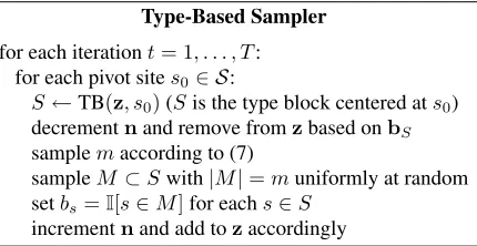
Type-Based Sampler

for each iterationt= 1, . . . , T: −for each pivot sites0∈ S:

−−S←TB(z, s0)(Sis the type block centered ats0)

−−decrementnand remove fromzbased onbS −−samplemaccording to (7)

−−sampleM⊂Swith|M|=muniformly at random −−setbs=I[s∈M]for eachs∈S

−−incrementnand add tozaccordingly

Figure 4: Pseudocode for the general type-based sampler. We operate in the binary variable representationbofz. Each step, we jointly sample|S|variables (of the same type).

sampler, we need to specify how to chooseS. Our general strategy is to first choose apivot sites0 ∈ S

uniformly at random and then setS =TB(z, s0)for

some function TB. CallSthetype blockcentered at s0. The following two criteria on TB are sufficient

for a valid sampler: (A)s0 ∈ S, and (B) the type

blocks arestable, which means that if we changebS

to anyb0_S(resulting in a newz0), the type block cen-tered ats0 with respect toz0 does not change (that

is, TB(z0, s0) = S). (A) ensures ergodicity; (B),

reversibility.

Now we define TB as follows: First setS ={s0}.

Next, loop through all sitess∈ Swith the same type ass0 in some fixed order, addings toS if it does

not conflict with any sites already in S. Figure 4 provides the pseudocode for the full algorithm.

Formally, this sampler cycles over |S| transition kernels, one for each pivot site. Each kernel (in-dexed by s0 ∈ S) defines a blocked Gibbs move,

i.e. sampling fromp(b_TB(z,s0) | · · ·).

Efficient Implementation There are two oper-ations we must perform efficiently: (A) looping through sites with the same type as the pivot sites0,

and (B) checking whether such a sitesconflicts with any site inS. We can perform (B) inO(1)time by checking if any element of∆zs:bs _{has already been} removed; if so, there is a conflict and we skips. To do (A) efficiently, we maintain a hash table mapping type t to a doubly-linked list of sites with type t. There is anO(1)cost for maintaining this data struc-ture: When we add or remove a sites, we just need to add or remove neighboring sitess0 from their re-spective linked lists, since their types depend onbs.

For example, in the HMM, when we remove sites, we also remove sitess−1ands+1.

For the USM, we use a simpler solution: main-tain a hash table mapping each wordw to a list of positions wherewoccurs. Suppose site (position)s straddles wordsaandb. Then, to perform (A), we retrieve the list of positions wherea,b, andaboccur, intersecting theaandblists to obtain a list of posi-tions where a b occurs. While this intersection is often much smaller than the pre-intersected lists, we found in practice that the smaller amount of book-keeping balanced out the extra time spent intersect-ing. We used a similar strategy for the PTSG, which significantly reduces the amount of bookkeeping.

Skip Approximation Large type blocks mean larger moves. However, such a blockSis also sam-pled more frequently—once for every choice of a pivot sites0 ∈ S. However, we found that

empir-ically, bS changes very infrequently. To eliminate

this apparent waste, we use the following approxi-mation of our sampler: do not considers0 ∈ S as

a pivot site ifs0 belongs to some block which was

already sampled in the current iteration. This way, each site is considered roughly once per iteration.4

Sampling Non-Binary Representations We can sample in models without a natural binary represen-tation (e.g., HMMs with with more than two states) by considering random binary slices. Specifically, suppose bs ∈ {1, . . . , K} for each site s ∈ S.

We modify Figure 4 as follows: After choosing a pivot site s0 ∈ S, letk = bs0 and choose k

0

uni-formly from{1, . . . , K}. Only include sites in one of these two states by re-defining the type block to beS = {s ∈ TB(z, s0) : bs ∈ {k, k0}}, and

sam-plebSrestricted to these two states by drawing from p(bS |bS ∈ {k, k0}|S|,· · ·). By choosing a random k0 each time, we allow b to reach any point in the space, thus achieving ergodicity just by using these binary restrictions.

5 Experiments

We now compare our proposed type-based sampler to various alternatives, evaluating on marginal

like-4

lihood (3) and accuracy for our three models:

• HMM: We learned a K = 45 state HMM on the Wall Street Journal (WSJ) portion of the Penn Treebank (49208 sentences, 45 tags) for part-of-speech induction. We fixedαr to0.1andµr to

uniform for allr.

For accuracy, we used the standard metric based on greedy mapping, where each state is mapped to the POS tag that maximizes the number of cor-rect matches (Haghighi and Klein, 2006). We did not use a tagging dictionary.

• USM: We learned a USM model on the Bernstein-Ratner corpus from the CHILDES database used in Goldwater et al. (2006) (9790 sentences) for word segmentation. We fixedα0to

0.1. The base distributionµ0penalizes the length

of words (see Goldwater et al. (2009) for details). For accuracy, we used word token F1.

• PTSG: We learned a PTSG model on sections 2– 21 of the WSJ treebank.5 For accuracy, we used EVALB parsing F1on section 22.6 Note this is a

supervised task with latent-variables, whereas the other two are purely unsupervised.

5.1 Basic Comparison

Figure 5(a)–(c) compares the likelihood and accu-racy (we use the term accuracyloosely to also in-clude F1). The initial observation is that the

type-based sampler (TYPE) outperforms the token-based sampler (TOKEN) across all three models on both metrics.

We further evaluated the PTSG on parsing. Our standard treebank PCFG estimated using maximum likelihood obtained 79% F1. TOKENobtained an F1

of 82.2%, and TYPE obtained a comparable F1 of

83.2%. Running the PTSG for longer continued to

5

Following Petrov et al. (2006), we performed an initial pre-processing step on the trees involving Markovization, binariza-tion, and collapsing of unary chains; words occurring once are replaced with one of 50 “unknown word” tokens, using base distributions{µr}that penalize the size of trees, and sampling the hyperparameters (see Cohn et al. (2009) for details).

6

To evaluate, we created a grammar where the rule proba-bilities are the mean values under the PTSG distribution: this involves taking a weighted combination (based on the concen-tration parameters) of the rule counts from the PTSG samples and the PCFG-derived base distribution. We used the decoder of DeNero et al. (2009) to parse.

improve the likelihood but actually hurt parsing ac-curacy, suggesting that the PTSG model is overfit-ting.

To better understand the gains from TYPE over TOKEN, we consider three other alterna-tive samplers. First, annealing (TOKEN_anneal) is a commonly-used technique to improve mixing, where (3) is raised to some inverse temperature.7 In Figure 5(a)–(c), we see that unlike TYPE,

TOKENanneal does not improve over TOKEN

uni-formly: it hurts for the HMM, improves slightly for the USM, and makes no difference for the PTSG. Al-though annealing does increase mobility of the sam-pler, this mobility is undirected, whereas type-based sampling increases mobility in purely model-driven directions.

Unlike past work that operated on types (Wolff, 1988; Brown et al., 1992; Stolcke and Omohun-dro, 1994), type-based sampling makes stochastic choices, and moreover, these choices are reversible. Is this stochasticity important? To answer this, we consider a variant of TYPE, TYPEgreedy: instead of sampling from (7), TYPEgreedy considers a type block S and sets bs to 0 for all s ∈ S if p(bS =

(0, . . . ,0)| · · ·) > p(bS = (1, . . . ,1) | · · ·); else

it setsbs to 1 for alls ∈ S. From Figure 5(a)–(c),

we see that greediness is disastrous for the HMM, hurts a little for USM, and makes no difference on the PTSG. These results show that stochasticity can indeed be important.

We consider another block sampler, SENTENCE, which uses dynamic programming to sample all variables in a sentence (using Metropolis-Hastings to correct for intra-sentential type-level coupling). For USM, we see that SENTENCE performs worse than TYPEand is comparable to TOKEN, suggesting that type-based dependencies are stronger and more important to deal with than intra-sentential depen-dencies.

5.2 Initialization

We initialized all samplers as follows: For the USM and PTSG, for each sites, we place a boundary (set bs= 1) with probabilityη. For the HMM, we setbs

to state 1 with probabilityηand a random state with

7

3 6 9 12 time (hr.) -1.1e7 -0.9e7 -9.1e6 -7.9e6 -6.7e6 log-lik eliho o d

3 6 9 12 time (hr.) 0.1 0.2 0.4 0.5 0.6 accuracy

2 4 6 8 time (min.) -3.7e5 -3.2e5 -2.8e5 -2.4e5 -1.9e5 log-lik eliho o d Token Tokenanneal Typegreedy Type Sentence

2 4 6 8 time (min.) 0.1 0.2 0.4 0.5 0.6 F1

3 6 9 12 time (hr.) -6.2e6 -6.0e6 -5.8e6 -5.7e6 -5.5e6 log-lik eliho o d

(a) HMM (b) USM (c) PTSG

0.2 0.4 0.6 0.8 1.0 η -7.1e6 -7.0e6 -6.9e6 -6.8e6 -6.7e6 log-lik eliho o d

0.2 0.4 0.6 0.8 1.0 η 0.2 0.3 0.4 0.5 0.6 accuracy

0.2 0.4 0.6 0.8 1.0 η -3.5e5 -3.1e5 -2.7e5 -2.3e5 -1.9e5 log-lik eliho o d

0.2 0.4 0.6 0.8 1.0 η 0.2 0.3 0.4 0.5 0.6 F1

0.2 0.4 0.6 0.8 1.0 η -5.7e6 -5.6e6 -5.6e6 -5.5e6 -5.5e6 log-lik eliho o d

(d) HMM (e) USM (f) PTSG

Figure 5: (a)–(c): Log-likelihood and accuracy over time. TYPEperforms the best. Relative to TYPE, TYPEgreedy tends to hurt performance. TOKENgenerally works worse. Relative to TOKEN, TOKENannealproduces mixed results.

SENTENCEbehaves like TOKEN. (d)–(f): Effect of initialization. The metrics were applied to the current sample after

15 hours for the HMM and PTSG and 10 minutes for the USM. TYPEgenerally prefers largerηand outperform the other samplers.

probability1−η. Results in Figure 5(a)–(c) were obtained by settingηto maximize likelihood.

Since samplers tend to be sensitive to initializa-tion, it is important to explore the effect of initial-ization (parametrized byη ∈[0,1]). Figure 5(d)–(f) shows that TYPE is consistently the best, whereas other samplers can underperform TYPE by a large margin. Note that TYPE favors η = 1in general. This setting maximizes the number of initial types, and thus creates larger type blocks and thus enables larger moves. Larger type blocks also mean more dependencies that TOKENis unable to deal with.

6 Related Work and Discussion

Block sampling, on which our work is built, is a clas-sical idea, but is used restrictively since sampling large blocks is computationally expensive. Past work for clustering models maintained tractabil-ity by using Metropolis-Hastings proposals (Dahl, 2003) or introducing auxiliary variables (Swendsen and Wang, 1987; Liang et al., 2007). In contrast, our type-based sampler simply identifies tractable

blocks based on exchangeability.

Other methods for learning latent-variable models include EM, variational approximations, and uncol-lapsed samplers. All of these methods maintain dis-tributions over (or settings of) the latent variables of the model and update the representation iteratively (see Gao and Johnson (2008) for an overview in the context of POS induction). However, these methods are at the core all token-based, since they only up-date variables in a single example at a time.8

Blocking variables by type—the key idea of this paper—is a fundamental departure from token-based methods. Though type-token-based changes have also been proposed (Brown et al., 1992; Stolcke and Omohundro, 1994), these methods operated greed-ily, and in Section 5.1, we saw that being greedy led to more brittle results. By working in a sampling framework, we were able bring type-based changes to fruition.

8

References

P. F. Brown, V. J. D. Pietra, P. V. deSouza, J. C. Lai, and R. L. Mercer. 1992. Class-based n-gram models of natural language. Computational Linguistics, 18:467– 479.

T. Cohn, S. Goldwater, and P. Blunsom. 2009. Inducing compact but accurate tree-substitution grammars. In

North American Association for Computational Lin-guistics (NAACL), pages 548–556.

D. B. Dahl. 2003. An improved merge-split sampler for conjugate Dirichlet process mixture models. Techni-cal report, Department of Statistics, University of Wis-consin.

J. DeNero, M. Bansal, A. Pauls, and D. Klein. 2009. Efficient parsing for transducer grammars. In North American Association for Computational Linguistics (NAACL), pages 227–235.

J. Gao and M. Johnson. 2008. A comparison of

Bayesian estimators for unsupervised hidden Markov model POS taggers. InEmpirical Methods in Natural Language Processing (EMNLP), pages 344–352. S. Goldwater and T. Griffiths. 2007. A fully Bayesian

approach to unsupervised part-of-speech tagging. In

Association for Computational Linguistics (ACL). S. Goldwater, T. Griffiths, and M. Johnson. 2006.

Con-textual dependencies in unsupervised word segmenta-tion. In International Conference on Computational Linguistics and Association for Computational Lin-guistics (COLING/ACL).

S. Goldwater, T. Griffiths, and M. Johnson. 2009. A Bayesian framework for word segmentation: Explor-ing the effects of context.Cognition, 112:21–54. A. Haghighi and D. Klein. 2006. Prototype-driven

learn-ing for sequence models. InNorth American Associ-ation for ComputAssoci-ational Linguistics (NAACL), pages 320–327.

P. Liang, M. I. Jordan, and B. Taskar. 2007. A

permutation-augmented sampler for Dirichlet process mixture models. InInternational Conference on Ma-chine Learning (ICML).

S. Petrov, L. Barrett, R. Thibaux, and D. Klein. 2006. Learning accurate, compact, and interpretable tree an-notation. In International Conference on Computa-tional Linguistics and Association for ComputaComputa-tional Linguistics (COLING/ACL), pages 433–440.

M. Post and D. Gildea. 2009. Bayesian learning of a tree substitution grammar. In Association for Com-putational Linguistics and International Joint Confer-ence on Natural Language Processing (ACL-IJCNLP). A. Stolcke and S. Omohundro. 1994. Inducing prob-abilistic grammars by Bayesian model merging. In

International Colloquium on Grammatical Inference and Applications, pages 106–118.

R. H. Swendsen and J. S. Wang. 1987. Nonuniversal critical dynamics in MC simulations. Physics Review Letters, 58:86–88.

J. G. Wolff. 1988. Learning syntax and meanings through optimization and distributional analysis. In