Lance Linton
B.Eng., M.Eng.College of Engineering and Science,
Victoria University
Submitted in fulfillment of the requirements of the degree of Doctor of Philosophy
Abstract
The huge demand of wireless communications has driven the require-ment for highly-efficient multiple-access communications schemes that can accommodate multiple simultaneous users, yet provide performance similar to single-user systems. Recently, iterative multiuser detection schemes have shown to provide this high level of performance at a manageable level of complexity. This thesis is concerned with iterative detection of two non-orthogonal asynchronous access schemes: code-division multiple-access (CDMA); and interleave-code-division multiple-access (IDMA).
A multi-rate IDMA system is developed where different users transmit data at different rates. High-rate users support multiple sub-streams, each coded as an IDMA layer. The iterative receiver treats each IDMA layer as a virtual user. Variance transfer analysis is employed to analyse the receiver performance, which is then optimised by developing a power allocation strategy. Simulation results demonstrate that the performance of this proposed system is close to the theoretical limit in a Rayleigh flat-fading environment.
Next, receiver performance is optimised by forward error correction code allocation. For multiuser systems with dynamic loads, new users are allocated codes according to the existing system load in order to optimise receiver convergence. Small multiuser systems have performances that approach the theoretical single-user bound.
number of users. In a Rayleigh flat-fading environment, simulation results show that the proposed scheme can outperform other common MIMO schemes and approaches within 0.25dB of the single-user bound.
The application of iterative multiuser detection to underwater acous-tic communications is considered next. Designing reliable communication systems for the underwater acoustic channel has proven to be very chal-lenging. A major channel impairment is the multipath interference caused by multiple reflections of the acoustic signal from the water surface and bottom. These reflections occur at small grazing angles and with small reflection losses, causing both long delay spread and large multipath amplitudes in the received signal.
The large delay-spread implies that single-carrier communication will be plagued by inter-symbol interference (ISI) that spans many symbols. As an alternative, multi-carrier modulation (MCM) has been proposed to increase the symbol interval and thereby decrease the ISI span. We combine Orthogonal Frequency-Division Multiplexing (OFDM), a low-complexity spectrally-efficient MCM technique, with an IDMA overlay to develop a multiple-access communications system that provides robust performance in the presence of large time-delay spread and the other impairments presented by the shallow water acoustic channel.
Declaration
I, Lance Linton, declare that this PhD thesis entitled “Iterative and Adaptive Processing for Multiuser Communication Systems” is no more than 100,000 words in length including quotes and exclusive of tables, figures, appendices, bibliography, references and footnotes. This thesis contains no material that has been submitted previously, in whole or in part, for the award of any other academic degree or diploma. Except where otherwise indicated, this thesis is my own work.
Acknowledgements
Nomenclature 1
1 Introduction 2
1.1 Multiple-Access Schemes . . . 3
1.2 Error Correction Coding . . . 5
1.2.1 Block Codes . . . 5
1.2.2 Convolutional Codes . . . 6
1.2.3 Concatenated Codes . . . 8
1.2.4 Turbo Codes . . . 9
1.3 Applications of Iterative Decoding . . . 11
1.4 Summary of Thesis Work . . . 12
1.4.1 Iterative Methods for Equalization and Multiuser Detection . . . 13
1.4.2 IDMA Performance Optimisation using Variance Transfer Analysis 14 1.4.3 Optimal Space-Time Coding using the Golden Code . . . 15
1.4.4 Multiuser Communications for Underwater Acoustic Channels . . 16
1.5 Original Contributions . . . 18
1.6 Thesis Outline . . . 19
1.7 Related Publications . . . 20
2 Iterative Decoding for Equalization and Multiuser Detection 22 2.1 Convolutional Coding for the Gaussian Channel . . . 24
2.1.1 Convolutional Encoding . . . 24
2.1.2 System Model . . . 27
2.1.3 Log Likelihood Ratios (LLRs) . . . 29
2.1.4 MAP Decoding using the BCJR Algorithm . . . 29
2.2 Intersymbol Interference (ISI) Channels . . . 36
2.2.1 System Model . . . 38
2.2.2 Optimal Detection . . . 41
2.3 Separate Equalization and Decoding for ISI Channels . . . 42
2.3.1 Trellis-Based MAP Symbol Detection . . . 44
2.3.2 Linear Equalization and Symbol Detection . . . 48
2.3.3 Trellis-Based MAP FEC Decoding . . . 52
2.3.4 System Performance . . . 55
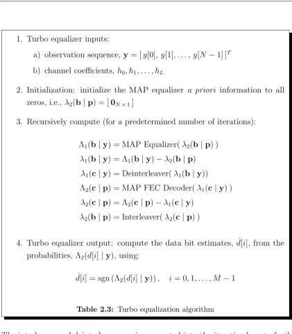
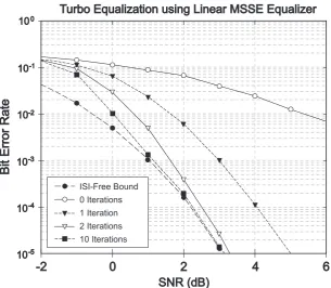
2.4 Turbo Equalization for ISI Channels . . . 57
2.5 Code Division Multiple Access (CDMA) and Multiuser Detection . . . . 63
2.5.1 Synchronous CDMA Signal Model . . . 64
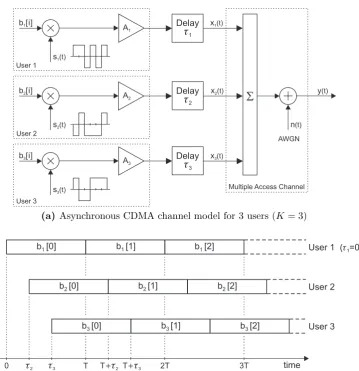
2.5.2 Asynchronous CDMA Signal Model . . . 65
2.5.3 Single-User Matched Filter Detector . . . 68
2.6 The Optimum Multiuser Receiver . . . 70
2.6.1 Synchronous Transmission . . . 70
2.6.2 Asynchronous Transmission . . . 71
2.7 Linear Multiuser Detectors . . . 74
2.7.1 Decorrelating Detector . . . 74
2.7.2 Minimum Mean-Square-Error Detector . . . 76
2.8 Turbo Multiuser Detection for Synchronous CDMA . . . 78
2.8.1 Optimal SISO Multiuser Detector . . . 81
2.8.2 Low-Complexity SISO Multiuser Detector . . . 82
2.9 Turbo Multiuser Detection for CDMA with Multipath Fading . . . 88
2.9.1 Signal Model and Sufficient Statistics . . . 89
2.9.2 SISO Multiuser Detector in Multipath Fading Channels . . . 93
2.10 Interleave-Division Multiple Access (IDMA) . . . 98
2.10.1 Transmitter Structure . . . 98
2.10.2 Iterative Receiver and Signal Model . . . 99
2.11 Conclusion . . . 103
3 IDMA Performance Optimisation using Variance Transfer Analysis 105 3.1 Variance Transfer Charts and Analysis . . . 107
3.1.1 ESE Variance Transfer Function . . . 107
3.1.2 FEC Decoder Variance Transfer Function . . . 109
3.1.3 Example Variance Transfer Chart . . . 109
3.2 Multi-Rate IDMA with Power Allocation . . . 111
3.2.1 Transmit Power Allocation . . . 113
3.3 FEC Allocation for Dynamic System Loads . . . 116
3.3.1 Simulation Results . . . 120
3.4 Conclusion . . . 120
4 Optimal Space-Time Coding using the Golden Code 123 4.1 Single-User MIMO System Model . . . 125
4.2 Space-Time Coding and Linear Dispersion Codes . . . 126
4.3 Decoding of Linear Dispersion Codes . . . 128
4.4 The Golden Code . . . 129
4.5 Single-User System Performance . . . 131
4.6 Multiuser MIMO System Model . . . 132
4.6.1 Multiuser Transmitter Structure . . . 132
4.6.2 Multiuser MIMO Signal Model . . . 134
4.6.3 Multiuser Iterative Receiver Structure . . . 136
4.7 Soft Multiuser Detector (MUD) . . . 137
4.8 Multiuser System Performance . . . 140
4.9 Conclusion . . . 142
5 Multiuser Detection for Delay-Spread Underwater Acoustic Channels 144 5.1 Channel Model . . . 145
5.1.1 Multipath Modeling . . . 146
5.1.2 Noise Modeling . . . 150
5.2 Single-Carrier IDMA for Multipath-Fading . . . 152
5.2.1 Transmitter Structure and Signal Model . . . 152
5.2.2 Iterative Receiver Structure . . . 153
5.3 Multi-Carrier IDMA (OFDM-IDMA) . . . 156
5.4 MIMO-OFDM-IDMA . . . 159
5.5 System Performance . . . 161
5.6 Conclusion . . . 164
6 Multiuser Detection for Doubly-Spread Underwater Acoustic Channels 166 6.1 Introduction . . . 167
6.2 Underwater Acoustic Channels and Channel Modelling . . . 170
6.2.1 Models for Channel Simulation . . . 171
6.2.2 Models for Channel Estimation . . . 172
6.3 Single-User Channel Equalization using the Kalman Filter . . . 179
6.3.2 Equalization of Channels with Known Coefficients . . . 181
6.3.3 Adaptive Equalization of Channels with Unknown Coefficients . . 184
6.4 Multiple Access IDMA . . . 186
6.4.1 Transmitter Structure . . . 186
6.4.2 Receiver Structure . . . 188
6.5 Multiuser Adaptive Soft EKF-Based Equalizer for Doubly-Spread Channels190 6.5.1 Multiuser System Model . . . 190
6.5.2 State-Space Model Incorporating A Priori Information . . . 192
6.5.3 Fixed-Lag Soft Input Extended Kalman Filtering . . . 195
6.5.4 Generating Extrinsic Information . . . 196
6.6 Performance Evaluation . . . 197
6.7 Conclusion . . . 204
7 Conclusion 206 7.1 Summary and Thesis Contributions . . . 207
7.1.1 IDMA Performance Optimisation using Variance Transfer Analysis 207 7.1.2 Optimal Space-Time Coding using the Golden Code . . . 208
7.1.3 Multiuser Communications for Underwater Acoustic Channels . . 209
7.2 Future Work . . . 211
Bibliography 214
List of Figures 227
Notation
R,Rn,Rn×m set of real numbers, vectors, and matrices C,Cn,Cn×m set of complex numbers, vectors, and matrices N∗ set of natural numbers {1,2,3. . .}
Q set of rational numbers
Z set of integers
? convolution
Hadamard product
⊗ Kronecker product
In n×n identity matrix
0n×m n×m zero matrix
{A}i,j i, j-th element of matrix A
AT transpose of matrix A
AH conjugate transpose of matrix A
A−1 inverse of matrix A
diag{a1, . . . , an} diagonal matrix with elements a1, . . . , an on the main diagonal
tr(A) trace of matrix A
arg maxxf(x) denotes the value of x that maximises f(x)
arg minxf(x) denotes the value of x that minimises f(x)
Cov{x, y} covariance of x and y δ(t) Dirac delta function E{x} expected value of x
exp{x} exponential function, exp(x) =ex
L(x) log likelihood ratio of x log(x) natural logarithm of x
N(µ, σ2) normal (Gaussian) distribution with mean µ and variance σ2
N(µ,C) multivariate normal distribution with mean µand covariance C p(x) probability density function of x
p(x|y) conditional probability density function of x conditioned on y P(x) probability mass function of x
P(x|y) conditional probability mass function of x conditioned on y
R{z},I{z} real and imaginary parts of z
sgn(x) signum function, sgn(x) = −1 ifx <0; sgn(x) = 1 if x >0 Var{x} variance of x
Commonly used symbols
Λ(x) a posteriori probability information in LLR form, Λ(x) = Lapp(x)
Λ1(·) a posteriori probability information (in LLR form) output from the soft equalizer or multiuser detector
Λ2(·) a posteriori probability information (in LLR form) output from the soft FEC channel decoder(s)
λ(x) extrinsic information in LLR form, λ(x) =Lext(x)
λ1(·) extrinsic information (in LLR form) output from the soft equalizer or soft multiuser detector, used as a priori information by the FEC channel decoder(s)
λ2(·) extrinsic information (in LLR form) output from the soft FEC channel decoder(s), used as a priori information by the soft equalizer or soft multiuser detector
b[i], bk[i] i-th bit (single-user case), i-th bit for the k-th user (multiuser case),
input to the symbol mapper or spreader (transmit side, coded or uncoded systems). b[i], bk[i] is coded and interleaved in coded systems
ˆb[i],ˆb
k[i] estimate of b[i], estimate of bk[i], output from the equalizer, detector,
or multiuser detector (receive side, coded or uncoded systems)
c[i], ck[i] i-th coded bit (single-user case), i-th coded bit for the k-th user
ˆ
c[i],cˆk[i] estimate of c[i], estimate ofck[i], input to the FEC decoder(s) (receive
side, coded systems)
d[i], dk[i] i-th input data bit (single-user case), i-th input data bit for thek-th
user (multiuser case), input to the FEC encoder(s) (transmit side, coded systems)
ˆ
d[i],dˆk[i] estimate of d[i], estimate of dk[i], output from the FEC decoder(s)
(receive side, coded systems)
K number of users in the multiuser system n(t) continuous-time channel noise at time t
x[i], xk[i] i-th transmitted symbol (single-user case), i-th transmitted symbol or
chip from user-k (multiuser case), discrete-time channel input
x(t), xk(t) transmitted signal at time t (single-user case), transmitted signal from
user-k at time t (multiuser case), continuous-time channel input y[i] i-th received symbol, discrete-time channel output
y(t) received signal at time t, continuous-time channel output Abbreviations
APP a posteriori probability
AR autoregressive
AR(p) autoregressive process of order p AWGN additive white Gaussian noise
BCJR Bahl, Cocke, Jelenik and Raviv (algorithm)
BEM basis expansion model
BER bit error rate
BI-AWGN binary-input additive white Gaussian noise
BPSK binary phase shift keying
CDMA code-division multiple-access
CE-BEM complex exponential BEM (discrete Fourier BEM)
DFE decision feedback equalizer
DFT discrete Fourier transform
DPSS discrete prolate spheroidal sequence (Slepian sequence)
ESE elementary signal estimator
EXIT extrinsic information transfer
FEC forward error correction
FFT fast Fourier transform
FIR finite impulse response
ICI inter-carrier interference
i.i.d independent and identically distributed
IDMA interleave-division multiple-access
ISI intersymbol interference
KF Kalman filter
K-L Karhunen-Loeve expansion
LD linear dispersion
LDPC low-density parity check
LLR log-likelihood ratio
MAI multiple-access interference
MAP maximum a posteriori probability
MCM multi-carrier modulation
MF matched filter
MIMO multiple-input multiple-output
ML maximum likelihood
MMSE minimum mean square error
MSE mean square error
MUD multiuser detection/detector
NKF nonlinear Kalman filter
OFDM orthogonal frequency division multiplexing
p.d.f probability density function
QAM quadrature amplitude modulation
QPSK quadrature phase shift keying
SISO soft-input soft-output
ST space-time
STBC space-time block code/coding
UAC underwater acoustic channel
US uncorrelated scattering
V-BLAST vertical Bell Labs layered space-time
VT variance transfer
WSS wide sense stationary
Introduction
The last two decades has witnessed a tremendous growth in wireless communications. Cellar mobile telephony and data services, and wireless networking were once rare but have become pervasive and an almost essential part of daily life. Future demand for these wireless devices and services show no sign of abating. In addition to the traditional network usage of wireless technology, the availability of low-cost wireless devices has enabled many new wireless applications over recent years. One notable application is distributed sensing, in which large numbers of inexpensive wireless nodes sense some ongoing process and wirelessly communicate with each other and wired access points. Environmental detection, surveillance, and health monitoring are just a few of the numerous potential uses of distributed sensor networks.
A defining feature of wireless communications is that all devices must share the electromagnetic spectrum in order to communicate with each other. Unlike in wired communications, where each communication channel could conceivably have a physical channel independent from all others, in wireless communication all channels come from a common medium. The scarcity of radio spectrum resource requires wireless communica-tion systems to reuse the frequency bands In order to achieve reliable communicacommunica-tions, some scheme must be developed for equitable sharing the usable frequencies. The issue of a large number of users sharing a single allocated spectrum in order to communicate is known as the multiple-access problem.
1.1 Multiple-Access Schemes
In a multiuser communication system, a large number of users share a common multiple-access channel to transmit information to a receiver. Multiple multiple-access systems generally require that when different transmitting sources are sending messages simultaneously through the same channel, the transmissions must be separated in some fashion so that they do not interfere with one another. This is usually accomplished by making the messages orthogonal to one another in the dimensions of frequency, time or code.
Frequency division multiple access (FDMA). In FDMA systems, the allocated fre-quency band is divided into non-overlapping sub-channels. Each transmitting source is assigned an individual sub-channel for data transmission, as shown in Figure 1.1a. A disadvantage of FDMA is that the frequency spectrum may not be used efficiently as no user can share the same frequency band at the same time and guard bands have to be maintained between adjacent signals spectra to minimise cross talk between sub-channels. FDMA also constrains the maximum bit rate per channel as increasing the bit rate requires the allocation of more frequency channels to a user.
Time division multiple access (TDMA). In TDMA systems, each user is allocated a unique cyclically repeating time slot within the channel. This allows a number of users to access and share a common channel without interfering with each other. Different users can transmit or receive messages, one after the next in the same bandwidth but in different time slots, as shown in Figure 1.1b. A disadvantages of TDMA is that it requires a significant amount of signal processing for synchronisation as the transmission of all users must be exactly synchronised. Additionally, TDMA needs guard times (the equivalent to guard bands in FDMA) between time intervals to reduce the effects of clock instabilities and transmission time delay.
Code-division multiple access (CDMA). CDMA is a spread-spectrum technique where the transmitted signal is spread over a wide frequency band, much wider that the minimum bandwidth required to transmit the information being sent.
or time, in a DS-CDMA system the users data are distinguished by the separation (cross-correlation) between their spreading sequences.
Code
Freq. Time
Channel 1
Channel 2
Channel 3
Frequency Bands
(a) FDMA
Time Slots Code
Freq. Channel 3 Time
Channel 2
Channel 1
(b) TDMA
Freq. Time
Code
Spreading Codes
3 l e n a h C
n 1 l e n a h C
n
2 l e n a h C
n
(c) CDMA
Figure 1.1: Multiple-access techniques: (a) Frequency-division multiple access (FDMA); (b) Time-division multiple access (TDMA); and (c) Code-division multiple access (CDMA).
CDMA schemes have become a very popular method for multiple-access communica-tions, and multiuser detection algorithms for CDMA receivers will be the focus of this thesis. Since the users in a DS-CDMA system are distinguished by the separation (cross-correlation) between their spreading sequences, we can categorise DS-CDMA schemes according to the cross-correlation between users, i.e.,
• orthogonal signalling - where the cross-correlation between all users is zero; or
• non-orthogonal signalling - where the cross-correlation between users is non-zero.
Additionally, CDMA schemes can also be categorised according to the synchronism of the users’ signals at the receiver, i.e.,
• synchronous schemes where the bit epochs of all the users are aligned at the receiver.
• asynchronous schemes where bit epochs of the users may be offset (not aligned) at the receiver.
Asynchronous schemes are also non-orthogonal because there are no known sets of spreading sequences that exhibit zero cross-correlation over a range of timing offsets.
where users are separated by unique interleaver sequences (instead of unique spreading sequences).
Iterative signal processing has proven to be an important technique in improving the performance of receivers in communications systems. Iterative techniques can be used to equalize inter-symbol interference channels (turbo equalization) and to resolve multiple-access interference (MAI) in multiuser receivers (turbo multiuser-detection, or turbo MUD). The origins of these techniques lie in error correction coding with the concepts of concatenated coding [29] and turbo codes. A brief review of error correction coding provides insight into the common building blocks of iterative processing.
1.2 Error Correction Coding
The approach to error correction coding taken by modern digital communication systems started in the late 1940’s with the ground breaking work of Shannon [107], Hamming [38], and Golay [34]. In his paper, Shannon developed the theoretical basis for coding which has become known as information theory. By mathematically defining the entropy of an information source and the capacity of a communications channel, he showed that it was possible to achieve reliable communications over a noisy channel provided that the source’s entropy is lower than the channel’s capacity. Shannon did not explicitly state how channel capacity could be practically reached, only that it was attainable.
1.2.1 Block Codes
Hamming is generally credited with discovering the first error correcting code [68] when, in 1946, he developed an algorithm that enabled early computers to correct isolated errors detected in the input data. His method was to group the data into sets of four information bits and then calculate three check bits which are a linearly combination of the information bits, resulting in a seven bit code word. After reading in a code word, the Hamming’s algorithm could detect errors and also determine the location of a single error. Hence, the Hamming code was able to correct a single error in a block of seven encoded bits.
only had the ability to correct a single error within the block. These issues were addressed by Golay, who generalized Hamming’s construction, and in the process, discovered two important codes: the binary Golay code; and ternary Golay code [137].
Reed-Muller (RM) codes [78] [99] were the next main class of linear block codes to be discovered, and were an important development because they allowed more flexibility in the size of the code word and the number of correctable errors per code word. They were followed by the discovery of cyclic codes, first discovered by Prange [90]. Cyclic codes are linear block codes that possess the additional property that any cyclic shift of a code word is also a code word. The cyclic property adds considerable structure to the code, which can be exploited by reduced complexity encoders and (more importantly) reduced complexity decoders. Important cyclic codes include the binary BCH codes [14] [43], and their non-binary extensions, the Reed and Solomon (RS) codes [100]. RS codes were a major advancement because their non-binary nature allows for protection against bursts of errors.
Although popular, block codes have two fundamental disadvantages: Firstly, their frame-oriented nature means that the entire code word must be received before decoding can be completed. This can introduce unacceptable latency into the system, particularly when block lengths are large. Secondly, most algebraic-based decoders for block codes work with hard-bit decisions, rather than with the unquantized, or “soft”, outputs of the demodulator. With hard-decision decoding, the output of the channel is taken to be binary, while with soft-decision decoding the channel output is continuous-valued [125].
In order to achieve the Shannon performance bound, a continuous-valued channel output is required. Block codes can achieve good performance over relatively benign channels, but they are generally power inefficient and have poor performance when the signal-to-noise ratio (SNR) is low. This poor performance at low SNR is not a function of the code itself, but is actually a function of the sub-optimality of hard-decision decoding. It is possible to perform soft-decision decoding of block codes, although historically soft-decision decoding has generally been regarded as too complex [125].
1.2.2 Convolutional Codes
of n output bits is a linear combination of the current set of m input bits and the bits stored in the shift register. The total number of bits that each output depends on is called theconstraint length, L. Therate,Rc, of the convolutional encoder is the number of data
bits m taken in by the encoder in one coding interval, divided by the number of code bits n output during the same interval, i.e., Rc=m/n. Just as the data is continuously
encoded, it can be continuously decoded with nominal latency. Additionally, the decoding algorithms can make full use of soft-decision information from the demodulator.
The first practical decoding algorithm for convolutional codes was the sequential decoder, introduced by Wozencraft and Reiffen [138]. However convolutional coding was not widely used until the introduction of the Viterbi algorithm (VA) [129], which was the first practical method for optimally (maximum likelihood) decoding convolutional codes.
de-interleaved data
1 2 3
7
4 5
8 9
6
interleaved data
1 2 3
7 4 5 8 9 6 Interleaver De-Interleaver -1 read write read input data
1 2 3 4 5 6 7 8 9
write
1 4 7 2 5 8 3 6 9
1 2 3 4 5 6 7 8 9
1 2 3
7 4 5 8 9 6 read Step 1.
Input (write) sequence
Step 2.
Output (read) sequence Interleaver Operation
De-Interleaver Operation
Step 1.
Input (write) sequence
Step 2.
Output (read) sequence
1 2 3
7
4 5
8 9
6
read
1 2 3
7
4 5
8 9
6 write
1 2 3
7
4 5
8 9
6
write
Figure 1.2: Block interleaver and de-interleaver operation
received code bits back in the proper order after demodulation and prior to decoding. By scrambling the order of the code bits at the transmitter, and then reversing the process at the receiver, burst errors can be spread out so that they appear independent to the decoder. The most common type of interleaver is the block interleaver (Figure 1.2), which is simply an Mb×Nb bit array. Data is placed into the array column-wise and
then read out row-wise. A burst error of length up to Nb bits can be spread out by a
block interleaver such that only one error occurs every Mb bits. There are also many
other interleaver types [130].
1.2.3 Concatenated Codes
Super Encoder
Outer Code Encoder input
data
Super Decoder
BPSK Modulator Inner Code
Encoder
(generally Reed-Solomon
Code)
(generally Convolutional
Code)
Outer Code Decoder
BPSK Demodulator Inner Code
Decoder
Channel
estimates of input
data
Super Channel
Deinterleaver p-1 Interleaver
p
(optional)
(optional)
Figure 1.3: Serial concatenated coding system. Optional interleaver and deinterleaver are used for channels with very long error bursts.
Convolutional codes and Reed-Solomon (RS) codes have complimentary properties. Convolutional codes are susceptible to burst errors, while RS codes can cope with burst errors quite well [137]. By concatenating an RS code and a convolutional code in series, Forney was able to take advantage of these complimentary properties and create an efficient system design for power-limited channels [29].
Hence, each decoder works with the appropriate type of data—the convolutional decoder works at low SNR with mostly independent errors, while the RS decoder works at high SNR with mostly burst errors. For cases with very long error bursts, a block interleaver can can be placed between the convolutional and RS encoders in order to spread long error bursts across several RS code words [137].
1.2.4 Turbo Codes
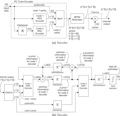
Although considerable progress had been made in coding theory, there was still a considerable gap between the performance of the best known codes and the theoretical limit predicted by Shannon. This changed when Berrou, Glavieux, and Thitimajshima [13] discovered turbo codes—a practical coding system that could approach Shannon’s
theoretical limit.
A turbo code is the parallel concatenation of two or more component codes. In its original form, the constituent codes were recursive systematic convolutional (RSC) codes [13], which are a subclass of convolutional codes. As shown in Figure 1.4a, two rate Rc = 1/2 RSC encoders work on the input data in parallel, with the input data
interleaved before being fed into the lower encoder (Code 2 encoder). The encoders are
systematic (one of the outputs is the input itself) and receive the same input (although in a different order), therefore, the systematic output of the Code 2 encoder is completely redundant and does not need to be transmitted. The overall code rate of the parallel concatenated code isRc= 1/3, although higher code rates can be obtained bypuncturing
(i.e., selectively removing) the parity output with a multiplexer (MUX) circuit [48].
systematic MUX Code 2 RSC Encoder input data d[i] Code 1 RSC Encoder d[i]
c [i](1)
c [i](2)
BPSK Modulator
Channel
{b [i],b [i],b [i]}(0) (1) (2)
{x [i],x [i],x [i]}(0) (1) (2)
{y [i],y [i],y [i]}(0) (1) (2)
Interleaver
p
AWGN n[i] channel output PC Turbo Encoderwhere: b [i] = d[i],(0) b [i] = c [i], b [i] = c [i] (1) (1) (2) (2) d [i]p
code 1 parity
code 2 parity (a) Encoder Code 1 MAP Decoder systematic Deinterleaver Interleaver
y [i](1) y [i](0)
y [i](2) DEMUX {y [i],y [i],y [i]}(0) (1) (2)
-1 hard decision Code 2 MAP Decoder d[i]^ extrinsic information
of code 1 decoder
extrinsic information
of code 2 decoder
information for code 2
decoder a priori information
for code 1 decoder
a priori
data bit estimates
code 2 parity code 1 parity
channel output L1(d[i]) l1(d[i]) l1(d [i])p
l2(d [i])p
Deinterleaver -1
Interleaver
l2(d[i]) L2(d [i])p
L
2(d[i]) information
of code 2 decoder a posterior
(b)Decoder
Figure 1.4: Parallel concatenated (PC) turbo encoder and decoder (systematic form).
However, iterative decoding obeys a law of diminishing returns and hence the incremental gain of each additional iteration is less than that of the previous iteration. It is the decoding method that gives turbo codes their name, since the feedback action of the decoder is similar to that of a turbo-charged engine [125].
Simulation results for the original turbo code of [13] showed that a bit error rate of 10−5 could be achieved at anE
performance with convolutional component codes could be matched or exceeded with block component codes [19] [94] [1]. As a result, it became clear that the real breakthrough from the introduction of turbo codes, was not the code construction, but the method of iterative decoding.
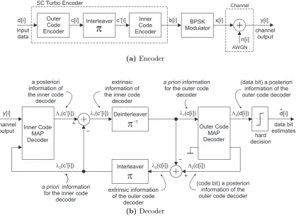
SC Turbo Encoder
Inner Code Encoder input data Outer Code Encoder BPSK Modulator Channel AWGN d[i] Interleaver
p
n[i]b[i] x[i] y[i]
channel output
c[i] c [i]p
(a) Encoder
channel output
(code bit) a posteriori information of the outer code decoder a posteriori
information of the inner code
decoder
Deinterleaver
Interleaver -1
L1(c [i])p
l1(c [i])p
l2(c [i])p
l1(c[i])
l2(c[i])
L2(d[i])
L2(c[i]) Inner Code MAP Decoder Outer Code MAP Decoder y[i] hard decision d[i] ^ data bit estimates information for the inner code
decoder
a priori
extrinsic information of the inner code
decoder
information for the outer code
decoder
a priori
extrinsic information of the outer code
decoder
(data bit) a posteriori information of the outer code decoder
(b)Decoder
Figure 1.5: Serial concatenated (SC) turbo encoder and decoder (non-systematic form).
1.3 Applications of Iterative Decoding
After the introduction of turbo codes, it was quickly recognized that the iterative decoding method was suitable for many other applications, and could be used as a general methodology for receiver design. Communication receivers typically consist of a cascade of subsystems, each optimized to perform a single task. Examples of these subsystems include equalizers, multiuser detectors, channel decoders, and source decoders.
of the processing chain do not benefit from information derived by stages further down the chain. The interface between stages can be greatly improved by using the same strategy devised to decode turbo codes. This general strategy of iterative feedback decoding or detection is termed turbo processing[66].
Turbo processing frameworks are constructed using soft-input soft-output (SISO) subsystems. A SISO subsystem receives decision values as input and produces soft-decision values as output. Soft-soft-decision values are passed down the chain and refined by subsequent stages. The soft-output of the final stage is then fed back to the first stage and the next iteration of processing is initiated. Multiple iterations of turbo processing can be performed, although, as with turbo codes, the incremental improvement in performance diminishes with each additional iteration.
Turbo processing can be used to combine channel decoding with source decoding [36], and channel decoding with symbol detection [66]. Other examples include:
Turbo equalization. This is a method of combining equalization with channel decoding [23]. An equalizer is a subsystem that compensates for the intersymbol interference (ISI) present in frequency selective channels. A frequency selective channel can be described as a rate-one convolutional code defined over the field of real or complex numbers. The combination of a convolutional channel code and ISI channel can be viewed as a serial concatenation of two convolutional codes, which is a type of serially concatenated turbo code, and can therefore can be decoded using the turbo decoding algorithm.
Turbo multiuser detection. Here, the concept of turbo processing is applied to coded multiple-access channels [44]. In a multiple-access channel, several users transmit at the same time and frequency, producing multiple access interference (MAI), which can be described as a form of time varying ISI. Thus, the multiple access channel can be viewed as a rate-one convolutional code with time varying coefficients taken over the field of real numbers. The combination of convolutional channel code and MAI channel can also be viewed as a serial concatenation of two convolutional codes, and is therefore suitable for turbo decoding.
1.4 Summary of Thesis Work
The first topic considers the optimisation of iteratively-decoded IDMA multiple-access communications systems. Using variance-transfer charts to analyse the performance of the iterative receiver, numerical methods are developed to maximise receiver performance by optimally allocating transmit power, and also dynamically allocating FEC codes for variable load systems. Optimal space-time coding (codes that provide both maximal spatial-multiplexing and diversity) are also investigated, and an efficient iterative multiuser receiver for the codes is developed.
The second topic considers the application of iteratively-decoded multiple-access communications in underwater acoustic network. We develop novel iterative receiver structures for underwater acoustic channels with delay-spread only, and with delay- and Doppler-spread (doubly-spread). Adaptive channel estimation for the doubly-spread channel is also developed.
1.4.1 Iterative Methods for Equalization and Multiuser Detection
An introduction and literature survey on applying the turbo principle to channel equal-ization and multiuser detection is presented.
Turbo Equalization. Equalization is the process of compensating for the effects of intersymbol interference (ISI) arising from the transmission of data over multipath delay-spread channels. We discuss the application of the turbo decoding algorithm to joint equalization and data detection.
Iterative Multiuser Detection. Multiuser detection (MUD) refers to the detection of data from multiple sources transmitting in a non-orthogonal multiple-access channel. For example, a CDMA system where users transmit using nonorthogonal spreading codes. We discuss the application of the turbo decoding algorithm to multiuser detection (MUD).
1.4.2 IDMA Performance Optimisation using Variance Transfer
Analysis
Variance Transfer (VT) charts [102] are used as a tool for analysing the iterative receiver performance. VT charts track the variance of the estimation error in the soft estimates that are exchanged between the multiuser detector (MUD) and the channel decoders, providing a graphical representation of the receiver’s convergence process. Although similar in concept to Extrinsic Information Transfer (EXIT) charts [115], VT charts are better suited for analysing multiuser detectors. Using variance transfer analysis, numerical methods are devised to optimise the receiver performance. Two multiuser system scenarios are considered for optimisation:
Layered IDMA with Power Allocation. Firstly, the IDMA concept is extended to a multi-rate system where different users transmit data at different rates and the same low-complexity iterative receiver structure can still be used. High-rate users are supported by breaking up the input data stream into multiple sub-streams. An IDMA layer is created from each sub-stream, and the multiple layers are then combined and the composite layered signal is transmitted from a single antenna. The iterative receiver treats each IDMA layer as a virtual user.
Chayat et. al. [18] observed that the performance of an iterative receiver is improved if different users transmit at different powers. This allows the iterative decoder to operate in an “onion peeling” mode, where the higher-power layers converge first, decreasing their contribution to the residual noise, and then the lower-power layers converge. CDMA and IDMA systems utilising iterative receivers can exploit this power allocation strategy to gain an improvement in performance.
To improve the performance of our layered IDMA scheme, we develop a simple power allocation scheme, where the power levels for each IDMA layer are calculated using Variance Transfer (VT) analysis and linear programming techniques. In a Rayleigh flat-fading environment, simulation results demonstrate that the performance of this proposed system is close to the theoretical limit.
manipulating transmit power, the judicious selection of FEC codes can also be used to optimise receiver performance.
A simple FEC code allocation strategy for multiuser systems with dynamic loads is devised. New users are allocated FEC codes according to the existing system load, providing optimal system performance over a range of operating conditions. We derive a numerical method for optimising performance based on FEC code allocation, and present simulation results. For small multiuser systems, results demonstrate that the performance of the proposed system approaches the theoretical single user bound.
1.4.3 Optimal Space-Time Coding using the Golden Code
Multiple antenna systems (commonly referred MIMO systems) have proven to be an effective method for realising high-rate reliable wireless communications. Generally coding strategies for MIMO systems has focused on providing either higher-rate or increased diversity over traditional single antenna systems. Layered space-time (BLAST) coding schemes utilise spatial multiplexing to achieve high-throughput rates, but do not provide any diversity gain. Orthogonal space time block coding (STBC) schemes provide diversity gain, but generally have coding rates of 1/2 or less.
Linear dispersion (LD) codes are a generalised class of space-time codes that can theoretically provide both diversity gain and high-rate [39]. Cyclic division algebra techniques have provided the means for constructing LD codes that provide both full-diversity and full-rate[105]. Space-time codes that achieve both full-full-diversity and -rate are known as perfect codes. The golden code[7] is a perfect code for 2×2 multiple-antenna systems.
We extend the golden code (GC) system to the multiuser case, and develop a MIMO-IDMA multiuser detector to decode LD codes. The performance of this GC-MIMO-IDMA scheme is compared against MIMO-IDMA schemes employing the Alamouti code and V-BLAST, and also against the single-user bound. In a Rayleigh flat-fading environment, simulation results show that GC-IDMA outperforms both Alamouti- and V-BLAST-IDMA at moderate and high signal to noise ratios. For an Eb/N0 ratio of 8dB or greater,
1.4.4 Multiuser Communications for Underwater Acoustic Channels
We consider the application of multiuser communications to underwater sensor networks. These networks enable a broad range of applications including environmental monitoring, undersea exploration, assisted navigation, and distributed surveillance [2]. Reliable high-performance sensor networks would need to be underpinned by a robust and efficient multiple-access underwater communications scheme.
Transmission of acoustic waves is considered the most practical means of underwater communications, as neither radio or optical systems have proved feasible. Radio systems are not feasible because only radio waves in the extra-low frequency range (<300Hz) are capable of propagating any distance through conductive sea water. Optical systems are also not suitable because optic waves, while not suffering as significantly from attenuation, are severely affected by scattering and absorption [110]. However, designing reliable underwater acoustic communications (UAC) systems has proven to be very challenging, with the underwater acoustic channel being referred to as “quite possibly natures most unforgiving wireless medium” [16].
Delay-spread underwater acoustic channels
One of the main channel impairments is multipath interference caused by multiple reflections of the acoustic signal from the water surface and bottom. These reflections occur at small grazing angles and with small reflection losses, causing both large delay-spread and large multipath amplitudes to be present in the received signal [51].
Large delay-spread implies that single-carrier communication will be plagued by inter-symbol interference (ISI) that spans many symbols. As an alternative, multi-carrier modulation (MCM) has been proposed to increase the symbol interval and thereby decrease the ISI span. In multi-carrier modulation, the data stream is split into several substreams and transmitted, in parallel, on different subcarriers. This transforms the inter-symbol interference (ISI)-inducing channel into a set of independent parallel subchannels. The principle advantage of multi-carrier schemes, relative to single-carrier schemes, is that they facilitate simple equalization of delay-spread channels. The is significant as equalization of underwater acoustic channels is usually a complex task.
data in parallel over a large number of orthogonal subcarriers. Typically, the number of subcarriers is chosen such that the symbol duration is large compared to the maximum delay of the channel, reducing the effects of ISI. However, to completely avoid the effects of ISI and thus, to maintain the orthogonality between the signals on the sub-carriers, a cyclic prefix (called a guard interval) is inserted between adjacent OFDM symbols. The guard time is chosen to be larger than the expected channel delay spread, such that multipath components from one symbol cannot interfere with the next symbol [28]. Maintaining subcarrier orthogonality eliminates intercarrier interference (ICI) and
therefore allow simple (low-complexity) data detection.
We combine Orthogonal Frequency Division Multiplexing (OFDM) with an IDMA overlay to develop a multiple-access communications system that provides robust perfor-mance in the presence of large time-delay spread and the other impairments presented by the shallow water acoustic channel. The proposed OFDM-IDMA scheme utilises a low-complexity iterative decoding algorithm based on the turbo-decoding concept. The experimental results demonstrate that the OFDM-IDMA scheme provides robust performance in delay-spread underwater acoustic environments.
Doubly-spread underwater acoustic channels
We extend the underwater acoustic channel to the doubly-spread case. The relative motion between the transmitter, receiver, and scattering objects imparts each path with a unique Doppler shift, so that multipath propagation also induces a frequency-domain spreading effect on the information signal. Such channels are both delay- and Doppler-spread (or equivalently, frequency- and time-selective), and are referred to as “doubly-spread” or “doubly-selective”.
guard interval) is much smaller than the channel coherence time (and hence the OFDM symbol length). But for rapidly TV channels, the OFDM symbol length would need to be made extremely short, at which point the loss of spectral efficiency due to guard insertion would be severe [104].
Therefore, we consider single-carrier system with adaptive channel-estimation for the doubly-spread underwater channel. A single-carrier system with linear traversal equalizer would face complexity issues due to the large number of equalizer taps required to compensate for the long delay-spread. Instead, a Kalman filter (KF) is used as equalizer. KF-based equalizers have been shown to perform significantly better than linear traversal equalizers at a much lower complexity (fewer equalizer taps) [55], [101]. Moreover, the state-space formulation of the Kalman equalizer is well suited for iterative receivers and allows easy incorporation of soft (a-priori) information for channel-coded systems.
The doubly-selective channels are modeled using basis expansion models (BEMs). A basis expansion model is a parsimonious (economical while accurate) low-rank channel model that exploits the inherent structure in the channel response [32]. Modelling of linear systems by basis functions can turn a time-varying system identification problem into a time-invariant one, thereby reducing the number of channel parameters to estimate and simplifying the equalization task.
The receiver uses a semi-blind iterative channel estimation algorithm to initially estimate the channels using only the pilot sequences and then iteratively includes the decoded data into the channel estimates to improve the estimation accuracy. Experimental results show that the proposed system provides robust performance in doubly-spread underwater acoustic environments.
1.5 Original Contributions
The original contributions of this research include:
• Simulation results illustrating the performance of the Golden Code over the wireless channels with Doppler spread.
• A novel power allocation method for multirate IDMA systems, where the power allocation is calculated using variance-transfer charts and linear programming.
• A novel FEC code allocation method to optimise multiuser system performance over varying system loads.
• The novel application of OFDM-IDMA to underwater acoustic communications and simulation results of the system performance.
• A novel iterative receiver for underwater acoustic communications for doubly-spread underwater channels. The iterative receiver incorporates a non-linear Kalman filter to perform joint decoding and channel equalization. Superimposed training is used for channel estimation and the time-varying channels are modeled using low-rank basis expansion models (BEMs).
These works were new when they were published or completed.
1.6 Thesis Outline
In this thesis, our goals are twofold. Firstly, we consider methods to multiuesr iterative receiver performance using power allocation, FEC code allocation, and maximising MIMO diversity through the use of perfect space-time codes. Secondly, we consider the application of underwater acoustic communications and develop multiuser receiver structures for channels with severe delay-spread and also doubly-spread. Therefore we organise the rest of the thesis as follows
In Chapter 2, we provide an introduction and literature survey on turbo equalization and turbo multiuser detection techniques. Detailed system models of iterative receivers for CDMA and IDMA multiple-access systems are also presented.
In Chapter 3, we describe our method of selecting transmit power levels to optimise the system performance. Next, we describe our method of assigning different FEC codes to different users to optimise the multiuser receiver performance. Both methods use variance transfer charts and linear programming.
In Chapter 5, we describe propagation models and noise models to characterise the underwater acoustic channel. Next, we describe a multiple-access system that combines Orthogonal Frequency Division Multiplexing (OFDM) with an IDMA overlay to provide robust performance in the presence of large time-delay spread and the other impairments presented by the shallow water acoustic channel.
In Chapter 6, we extend our underwater channel model to include both delay- and doppler-spread, so-called doubly-spread channel. Next, we describe our multiuser receiver for doubly-spread channels. This is an iterative receiver that uses soft-input soft-output Kalman filter as an adaptive MIMO equalizer. The time-varying characteristics of the channel are modeled using low-rank basis expansion models.
In Chapter 7, we summarise the thesis work, state its major contributions, and finally suggest some possible future directions
1.7 Related Publications
Part of the thesis work have been published in major conferences or journals related to wireless communications or underwater acoustic oceanic communications. Below is an incomplete list:
Related Publications of Chapter 3 include:
• L. Linton, P. Conder, and M. Faulkner, “Multi-Rate Communications Using Layered Interleave-Division Multiple Access with Power Allocation,”2009 IEEE Wireless Communications and Networking Conference, WCNC 2009, 5-8 April 2009,
Bu-dapest, Hungary
• L. Linton, P. Conder, and M. Faulkner, “Improved Interleave-Division Multiple Access (IDMA) Performance Using Dynamic FEC Code Allocation,”2010 IEEE Wireless Communications and Networking Conference, WCNC 2010, 18-21 April 2010, Sydney, Australia
Related Publications of Chapter 4 include:
on Signal Processing and Communication Systems, ICSPCS-2007 17-19 December 2007, Gold Coast, Australia
• L. Linton, P. Conder, and M. Faulkner, “Multiuser MIMO Communications using Interleave-Division Multiple-Access and Golden Codes,” 2008 IEEE 67th Vehicular Technology Conference: VTC2008-Spring 11-14 May 2008, Marina Bay, Singapore
Related Publications of Chapter 5 include:
• L. Linton, P. Conder, and M. Faulkner, “Multiuser Communications for Underwater Acoustic Networks using MIMO-OFDM-IDMA,” 2nd International Conference on Signal Processing and Communication Systems, ICSPCS-2008, 15-17 December 2008, Gold Coast, Australia
• L. Linton, P. Conder, and M. Faulkner, “Multiple-Access Communications for Underwater Acoustic Sensor Networks using OFDM-IDMA,”MTS/IEEE Oceans 2009 Conference, 26-29 October 2009, Biloxi, Mississippi, USA
Related Publications of Chapter 6 include:
Iterative Decoding for Equalization and
Multiuser Detection
In this chapter, the turbo decoding principle is applied to the communications problems of channel equalization and multiuser detection. These fundamental techniques are the basis for the research described in the the subsequent chapters of this thesis.
First, convolutional coding over an AWGN channel is introduced. Convolutional codes are trellis-based (or state-machine based) codes that are commonly used for forward error correction (FEC) and are also a fundamental building block of iterative communication systems. An optimal decoding method for convolutional codes is the BCJR MAP algorithm which decodes the transmitted data by estimating the most probable state transitions of the encoder from the received (noisy) channel observations.
Next, the intersymbol interference (ISI) channel is presented. The traditional methods of data protection used in FEC do not work well when the channel over which the data is sent introduces additional distortions in the form of ISI. When the channel is bandlimited of for other reasons is time-dispersive in nature, then the receiver will generally need to compensate for the channel effects prior to employing a standard decoding algorithm for the FEC. Such methods for channel compensation are typically referred to as channel equalization .
One approach to the problem of coded transmission over an ISI channel is to consider the channel as a rate-1 convolutional code and consequently the time dispersion of the channel can be considered to be equivalent to the shift register elements of the convolutional encoder. The FEC encoder of the transmitter and the ISI channel can then
be thought of as an example of Forney’s serial concatenated coding scheme transmitting over a memoryless AWGN channel.
However, when the super-trellis of the combined states of the FEC encoder and ISI channel is constructed, it becomes apparent that the complexity of an optimal joint FEC and channel trellis decoder would be excessive for practical implementations. Therefore, suboptimal detection methods must be considered. For complexity reasons, the problems of FEC decoding and channel equalization have traditionally been considered separately, with limited interaction between the two blocks. As such, substantial performance degradation is typically induced through the separation of these inherently dependent tasks.
Recently, research in iterative methods for equalization, generally referred to as turbo equalization, has enabled feasible approaches to jointly solving the equalization and decoding tasks. As a result, the performance gap between optimal joint decoding and equalization and that achievable through systems with practical complexity has been narrowed in a manner similar to that of near Shannon-limit communications using turbo codes [12].
2.1 Convolutional Coding for the Gaussian Channel
Convolutional codes are stream-oriented linear codes and are a building block of turbo code, turbo equalization, and turbo multiuser detection schemes. A convolutional encoder assigns code bits to an incoming information bit stream continuously, in a stream-oriented fashion. The convolutional code is named after its encoding method of using modulo-2 convolutions to generate the redundant bits.
2.1.1 Convolutional Encoding
The role of the encoder is to take the binary data sequence to be transmitted as input and produce an output that contains not only this data but also additional redundant information that can be used to protect the data from the possibility of errors that might occur in the data stream as a result of additive noise in the transmission or detection errors at the receiver.
A convolutional encoder can be represented by a finite-state machine, taking in a continuous stream of message bits and producing a continuous stream of output bits. The encoder has a memory of the past inputs, which is held in the encoder state. The output depends on the value of this state, as well as on the present message bits at the input, but is completely unaffected by any subsequent message bits.
The encoder memory is generally implemented using a linear finite-state shift register circuit where each shift register element represents a time delay of one unit. The bit at the output of the shift register element at time iis the bit that was present at the input of the element at time i−1. The set of all the shift registers elements together holds the encoder state. An encoder can have one or more shift registers, one or more inputs and one or more outputs.
Consider the convolutional encoder of Figure 2.1a. The serial-to-parallel converter splits the input message into vectors of m-bits length, i.e., d[i] =d(1)[i], . . . , d(m)[i]T. At each state transition, i, the encoder receives a m-bit input vector and outputs a n-bit coded vector,c[i] =
c(1)[i], . . . , c(n)[i]T
. The parallel-to-serial converter generates the output coded bit stream by concatenating the coded vectors c[i] from each state transition. The convolutional code is said to have rate Rc =m/nif, at each time instant
Convolutional Encoder
S P
P S
(1)
d[i] c[i]
d [i]
(m) d [i]
(1) c [i]
(n) c [i]
(a)Encoder schematic block
D D
s(1) s(2)
(1)
d [i]
(1)
c [i]
(2)
c [i]
(b) Example rate-1/2 encoder circuit
Figure 2.1: Convolutional encoder schematic block code, and example rate-1/2 encoder for generator polynomial (1 +D2,1 +D+D2).
Without loss of generality, we consider the case where the input to the convolutional encoder is a single-bit vector, i.e., m = 1. For an input message of block length M,
{d[i]}M−1
i=0 , the output coded message will have a block length ofN = nM, i.e., {c[i]}
N−1
i=0 . Figure 2.1b shows an example binary convolutional encoder, whereD represents the delay elements (shift register elements), and⊕ represents modulo-2 addition. At time i the input to the encoder is one message bitd(1)[i] and the output is a two-bit vector, c[i] = [c(1)[i], c(2)[i] ]T; thus the code rate is 1/2. The state of this encoder is given by
S = (s(1), s(2)), where s(1) ∈ {1,0} and s(2) ∈ {1,0} are the contents of the left-hand register element and the right-hand register element, respectively. Thus the encoder can be in one of four possible states, S0 = (0,0), S1 = (0,1), S2 = (1,0), and S3 = (1,1). As there is only one input, the message d is simply given by [d(1)[0], . . . , d(1)[M −1] ], and therefore the superscript (1) can be dropped.
For the example encoder shown in Figure 2.1b, the output bitsc(1)[i] and c(2)[i] (at time i) are computed as:
c(1)[i] =d[i]⊕s(2)[i] and c(2)[i] =d[i]⊕s(1)[i]⊕s(2)[i] (2.1)
where ⊕ represents modulo-2 addition. The equations in (2.1) can be more concisely represented by the generator polynomial (1 +D2,1 +D+D2), where D is equivalent to the discrete-time delay operator z−1.
must be zero, which implies a small rate loss. This loss can be controlled by using long sequences (i.e., large values of M), or can be avoided by using tail-biting encoding [136] [48].
Since a convolutional encoder can be thought of as a finite-state machine, the encoder behaviour can be described by a state diagram which portrays the temporal relationships between inputs, states and outputs. This representation is often helpful for both encoding and decoding purposes. For an encoder with L memory elements (i.e.,L shift register elements), there are 2L encoder states in the state diagram. The state diagram in Figure 2.2a provides a graphical representation of the state transitions of the encoder in Figure 2.1b. Each of the four states is represented by a node. The edges between nodes represent the possible state transitions. Each edge is labeled with the input bit that produced the transition and the output bits generated.
0/00 1/01 0/11 1/11 1/10 0/10 1/00 0/01 S (0,0) 0 S (1,1) 3 S (1,0) 1 S (0,1) 2
(a) State diagram
S 3 S 2 S 1 S 0
time = i-1
S 3 S 2 S1 S 0 S3 S 2 S 1 S 0 1/10 0/00 0/10 1/00 1/11 0/1 1 1/01 0/01 1/10 0/00 0/10 1/00 1/11 0/1 1 1/01 0/01 i i+1
(b) Trellis diagram
Figure 2.2: State diagram and trellis representations of the convolutional code of Figure 2.1b. The trellis states correspond to the content of the delay elements asS0= (0,0),
S1 = (1,0), S2= (0,1) and S3 = (1,1).
Although the state diagram describes the convolutional encoder state and input-output relationship completely, it does not provide a record of how the state has evolved with time. For this we use a trellis diagram. Figure 2.2b shows the state diagram expanded in time to produce a trellis segment. On the left each state is represented for time i and on the right a copy of each state is represented for time i+ 1. The state transition edges are joined from a state at time i to a state at time i+ 1 to show the changes with time. Each path through the trellis is an evolution of the convolutional encoder for one of the 2M possible input streams. Consequently the set of codewords for a convolutional code
This trellis representation enables optimal decoding of convolutional codes with reasonable complexity. Each path in the trellis corresponds to a codeword, and so the maximum likelihood (ML) decoder (which finds the most likely codeword) searches for the most likely path in the trellis. Alternatively, each edge in the trellis can correspond to a particular input: the bit-wise maximum a posteriori (MAP) decoder, which searches for the maximum-probability input bit, calculates the probability of each trellis edge [48].
2.1.2 System Model
Conv. Encoder
S P
P S
MAP Decoder Symbol
Mapper
d[i] d[i]
Transmitter Receiver
AGWN n[i] BI-AWGN Channel
h0 Channel Coefficient (1)
c [i]
(n) c [i]
y [i](1)
y [i](n)
x[i] y[i]
c[i]
0 -1 +1 1
Figure 2.3: System model for a coded transmission over a memoryless AWGN channel
Figure 2.3 shows the system model for a convolutional-coded transmission scheme. The input data sequence d= [d[0], d[1], . . . , d[M−1] ]T is encoded by the convolutional encoder (with rate Rc) generating a n-bit coded vector, c[i], for each data bit, d[i], i.e.,
c=cT[0], cT[1], . . . , cT[M−1]T where c[i] =c(1)[i], . . . , c(n)[i]T (2.2)
The parallel-to-serial converter (P/S) concatenates M of thec[i] vectors to form aN-bit frame. Hence, (2.2) can be restated as c= [c[0], c[1], . . . , c[N −1] ]T, where N is the
frame length (N = nM), and the elements of c are referred to as coded bits. The coded bit sequence c is then BPSK modulated, producing the symbol sequence x, which is defined as
x= [x[0], x[1], . . . , x[N−1] ]T (N×1 vector) (2.3)
where x[i]∈ {+1,−1}. Finally, the sequence of BPSK symbols is transmitted over an AWGN channel. The decoder receives a noisy version of the transmitted symbol sequence from which to determine the message. The sequence of noise-corrupted symbols received from the channel are denoted by
The serial-to-parallel converter (S/P) divides the received symbol sequence intoM vectors of n-bits length, i.e.,
y=yT[0],yT[1], . . . , yT[M −1]T where y[i] =y(1)[i], . . . , y(n)[i]T (2.5)
At each state transition, i, the MAP decoder receives a n-bit input vector y[i], and outputs the message bit estimate ˆd[i]. After M state transitions of the MAP decoder, the estimated message sequence can be formed as dˆ= [ ˆd[0],d[1], . . . ,ˆ d[Mˆ −1] ].
We consider the binary-input additive white Gaussian noise (BI-AWGN) channel, which is both symmetric and memoryless. A binary-input channel is symmetric if both input bits, {+1,−1}, are corrupted equally by the channel. A channel is considered
memoryless if the channel output at any time instant depends only on the input at that time instant, and not on previously transmitted symbols. This property can be expressed in terms of channel transition probabilities as
p(y|x) =
N−1
Y
i=0
p(y[i]|x[i]) (2.6)
where xis the transmitted symbol sequence defined in (2.3), andyis the received symbol sequence defined in (2.4). A memoryless channel is therefore completely described by its input and output alphabets and the conditional probability distribution p(y|x) for each input-output symbol pair.
The BI-AWGN channel of Figure 2.3 can be described by the equation
y[i] =h0x[i] +n[i] (2.7)
where x[i] ∈ {−1,+1} is the i-th transmitted symbol, y[i] is the i-th received symbol and n[i] is the additive noise sampled from a Gaussian random variable with zero mean and σ2 variance, i.e., n[i]∼ N(0, σ2). The probability density function for n is
p(n) = √ 1
2πσ2 exp
− n
2 2σ2
, (2.8)
where exp(·) is the exponential function. If the source is equiprobable then P(x[i] =
−1) =P(x[i] = +1), then we have for the BI-AWGN channel:
p(y[i]|x[i] = ±1) = √ 1
2πσ2 exp
− 1
2σ2 (y[i]∓h0) 2
2.1.3 Log Likelihood Ratios (LLRs)
When using probabilistic decoding methods (such as the BCJR algorithm) on binary codes, the probabilities input and output from the decoder are often expressed in log likelihood ratio (LLR) form.
For a binary variable x, the probabilitiesP(x= 1) givenP(x= 0) are related since P(x= 1) = 1−P(x= 0). Therefore only a single value is needed in order to represent the set of probabilities for x. The log likelihood ratio (LLR) is used to represent the probability metrics for a binary variable by a single value, and is given by
L(x) = logP(x= 0)
P(x= 1) (2.10)
The sign of L(x) provides a hard decision on x and the magnitude |L(x)| gives the reliability of this decision. In iterative decoding, a posteriori probability (APP) LLRs are commonly denoted Λ(·), i.e., Λ(x) =Lapp(x). Similarly, extrinsic information LLRs
are commonly denoted λ(·), i.e., λ(x) = Lext(x). LLRs can be translated back to
probabilities as follows:
P(x= 1) = exp{−L(x)} 1 + exp{−L(x)} =
1 2
1−tanh
L(x) 2
(2.11)
and
P(x= 0) = exp{L(x)} 1 + exp{L(x)} =
1 2
1 + tanh
L(x) 2
(2.12)
A benefit of the logarithmic representation of probabilities is that when probabilities need to be multiplied, log-likelihood ratios need only be added; which can reduce implementation complexity.
2.1.4 MAP Decoding using the BCJR Algorithm
Since the convolutional encoder has memory, the codeword bit output at timei is influenced by the codeword bits sent before it and may itself influence the codeword bits sent after it. Thus all the bits in y may tell us something about the message bit at time i. To incorporate the information from both the bits transmitted before time i and the bits transmitted after timei, the BCJR decoding uses two passes through the trellis:
• a forward pass that provides the current message bit on the basis of only the codeword bits that were transmitted before it; and
• a backward pass that predicts the current message bit on the basis of only the codeword bits that were transmitted after it.
Since the message bits are the input to a binary convolutional encoder we can determine which message bit was sent by finding out which state transition occurred. We denote:
• S as the set of possible states,
• T+ as the set of state transitions (S
r, Ss) that correspond to a 1 input bit,
• T− as the set of state transitions (S
r, Ss) that correspond to a 0 input bit, and
• T as the set of all valid state transitions (Sr, Ss), i.e.,T =T+∪ T−.
For example, the convolutional encoder in Figure 2.1b has S ={S0, S1, S2, S3},
T+ ={(S
0, S1),(S1, S3),(S2, S1),(S3, S3)}, (2.13)
T− ={(S0, S0),(S1, S2),(S2, S0),(S3, S2)}, and (2.14)
T ={(S0, S0),(S0, S1),(S1, S2),(S1, S3),(S2, S0),(S2, S1),(S3, S3),(S3, S2)}. (2.15)
The probability that d[i] was 1 is the probability that a state transition in the set T+ occurred at time i:
P(d[i] = 1|y) = X (Sr,Ss)∈T+
P(ψi =Sr, ψi+1 =Ss|y) (2.16)
where ψi is the variable for the state at time i, andS ={S0, S1, . . . , S(2L−1)} is the set
of possible values that the state can take. We represent by Sr andSs the values of the
the probability that a state transition in the set T− occurred at time i:
P(d[i] = 0|y) = X (Sr,Ss)∈T−
P(ψi =Sr, ψi+1=Ss |y) (2.17)
For convenience, P(ψi = Sr) will be denoted as P(Sr), and P(ψi+1 = Ss) denoted as
P(Ss) when the context is clear.
Thus determining the message bit probabilitiesP(d[i]|y) requires that we determine the probability of each state transition,P(Sr, Ss |y), given that we have only the received
vectory. Using Bayes’ rule we can rewrite P(Sr, Ss|y) as
P(Sr, Ss|y) =
p(Sr, Ss,y)
p(y) (2.18)
Substituting (2.18) into equations (2.16) and (2.17), the log-likelihood ratio (LLR) for bit d[i] can be defined as
Λ(d[i]|y) = log
P
(Sr,Ss)∈T+ p(Sr, Ss,y)
P
(Sr,Ss)∈T− p(Sr, Ss,y)
(2.19)
Note that the termp(y) in (2.18) cancels out when the ratio is taken, and therefore does not need to be explicitly calculated.
To enable the efficient calculation ofp(ψi, ψi+1,y), the received vector, y, is split into three sets:
p(ψi, ψi+1,y) = p(ψi, ψi+1,y−[i],y[i],y+[i]) (2.20)
where
• y−[i] represents the values received for the set of bits sent before time i;
• y[i] represents the values received for the set of bits sent at time i; and
• y+[i] represents the values received for the set of bits sent after time i.
Applying Bayes’ rule again,
p(ψi, ψi+1,y) = p(ψi, ψi+1,y−[i],y[i],y+[i])
=p(ψi,y−[i])p(ψi+1,y[i]|ψi,y−[i])p(y+[i]|ψi, ψi+1,y−[i],y[i])
Since a convolutional encoder has been used to generate the codeword bits, we know that the codeword bits output at time iare completely determined by the state transition, ψi (at time i) to ψi+1 (at time i+ 1). Also, since we are considering a memoryless channel, the channel output y[i] depends only on the transmitted codeword bit c[i] and the channel noise at time i, and is not affected by anything previously or subsequently transmitted through the channel. Putting these together, if we know the probability of the state transition ψi to ψi+1 then the probability of y[i] is completely independent of y+[i] and y−[i], and so
p(ψi+1,y[i]|ψi,y−[i]) = p(ψi+1,y[i]|ψi).
Similarly, if we know the probability of the encoder state at time ithen the probability of y+[i] is independent of both the past states and past outputs and so
p(y+[i]|ψi, ψi+1,y−[i],y[i]) =p(y+[i]|ψi+1).
Thus finally
p(ψi, ψi+1,y) =p(ψi,y−[i])p(ψi+1,y[i]|ψi)p(y+[i]|ψi+1). (2.21)
The BCJR algorithm assigns a label to each term in (2.21), therefore (2.21) can be restated as [48]
mi(ψi, ψi+1) = αi(ψi)γi(ψi, ψi+1)βi+1(ψi+1) (2.22)
where
mi(ψi, ψi+1) =p(ψi, ψi+1,y), (2.23) αi(ψi) =p(ψi,y−[i]), (2.24)