A Long Short-term Traffic Flow Prediction Method
Optimized by Cluster Computing
Boyi Liu1,4 , Jieren Cheng1,3, Qiang Liu2, and Xiangyan Tang1,* 1 Hainan University, 570228, Haikou, China; [email protected]
2 College of Computer, National University of Defense Technology, Changsha, 410073, China;
3 State Key Laboratory of Marine Resource Utilization in South China Sea, Hainan University, 570228, Haikou,
China; [email protected]
4 University of Chinese Academy of Science, 100000, Beijing, China; [email protected]
* Correspondence: [email protected], [email protected]; Tel.: +86 15108910688
Abstract:Accurate and fast traffic flow forecasting is vital in intelligent transportation system because many of the advanced features in intelligent transportation systems are based on it. However, existing methods have poor performance regarding accuracy and computational efficiency in long-term traffic flow forecasting under big data. Hence, we propose an improved Long short-term memory (LSTM) Network and its cluster computing implementation in this paper to address the above challenge. We propose a singular point probability LSTM (SDLSTM) algorithm. The method discards the units of the network according to the singular point probability during the training process and amends the SDLSTM by Autoregressive Integrated Moving Average Model (ARIMA) to achieve the accurate prediction of 24-hour traffic flow data. Furthermore, the paper designs a scheme for implementing this method through cluster computing to shorten the calculation time and improve the system’s operating speed. Theoretical analysis and experimental results show that SDLSTM gains a higher accuracy rate and better stability in the long-term traffic flow forecasting compared with previous methods.
Keywords:traffic flow forecasting; cluster computing;LSTM neural networks
1. Introduction
With the development of social economy and transportation, traffic problems appear more frequently. There is great potential for development of crowdsourcing for mobile networks and IoT [1,2] in transportation. The traditional mode of transport has encountered more and more challenges, attracted worldwide attention. In recent years, many countries have invested lots of manpower and resources to carry out the development of management and control technology in the road transportation system. With the development of crowdsourcing for mobile networks and IoT, ITS (Intelligent Transportation System) has been developed rapidly [3,4]. Accurate traffic flow forecasting is the prerequisite and the key step to realize ITS, it is conducive to improving the efficiency of transport operations and the quality of people’s travel. Traffic flow forecasting is also helpful to alleviate the road congestion, reduce carbon emissions, and conserve the energy and so on. Especially with the rapidly development of big data technology, some methods predict the traffic flow data and plan the vehicle travel path relying on the current and historical traffic flow data. These methods forecast the traffic flow reasonably and designed the best route for vehicles, realizing the traffic’s balanced distribution in the road network and improving road utilization. The longer the time of traffic flow prediction, the greater the value of its utility. However, the current researches are mainly to solve the short-term traffic flow forecasting problem. Accuracy of the long-term traffic flow forecasting is low. The paper made a research on this problem and proposed a new traffic flow prediction algorithm with higher accuracy and longer prediction time. It will be popular if combined with the crowdsourcing for Mobile Networks and IoT.
Traffic flow is an important measure of the state of the road network. It refers to the number of vehicles through a road section during a period of time [5]. The excellent traffic flow prediction algorithm can predict the traffic flow data for a certain period of time earlier and more accurately. Traffic flow data is affected by many factors, for example the noise and some non-linear interferences. So, its rule is difficult to grasp, especially in the long-term traffic flow forecast [6], which has been a difficult point. In recent years, many traffic flow prediction algorithms have been proposed [7,8]. They can be broadly divided into two categories according to their forecasting basis: one prediction model is based on mathematical statistics and traditional mathematical such as calculus [9]; the other is a
prediction model based on modern science and technology methods [10].
The first class certainly includes many traffic flow prediction algorithms. One of the representative results is the time-series model [11] used in the traffic flow prediction field for the first time by Ahmed
and Cook in 1979. It includes the auto regressive model (AR) [12], the moving average model (MA)
[13], and the auto regressive moving average model (ARMA) [14]. The technology is matured and has
high accuracy when the sample data is sufficient. It is usually used in relatively stable traffic perdition. The method required a lot of uninterrupted data and it is easily to be interfered by random factors.
Stephanedes proposed History Average Model [15] applied to urban traffic control system in 1981. The
algorithm is simple and fast but cannot cope with emergencies. Okutani and Stephanedes proposed Kalman Filtering Model [16] for the traffic flow’s prediction in 1984, its predictive factor selection is flexibility and has high precision and good robustness. However, this method requires a lot of matrix calculations and its forecast value is delayed for several time periods sometimes, which making it difficult to realize real-time online prediction. In addition, a series of traffic flow forecasting methods have been proposed in recent years, spatial-temporal characteristics-based analysis [17], random forest model [18] and similarity model [19], etc.
Crowdsourcing for mobile networks and IoT has widely used in the second class of traffic prediction methods. One of the representative traffic flow prediction algorithm of the second class is
Davis and Nihan’s Nonparametric Regressive Model [20] applied to traffic flow prediction in 1991.
Without prior knowledge, it can perform more accurate than parametric modeling only with sufficient historical data, but its complexity is also high. Dougherty proposed neural network [21] for traffic flow prediction in 1995, which is suitable for complex and non-linear conditions, and it can be effective to predict when the data is incomplete and inaccurate with good adaptability and fault-tolerance, but it requires a lot of learning data and the training process is complex; The classification regression tree method [22] for the traffic flow forecast proposed by Xu Yanyan et al. in 2013 has a better prediction effect and interpretability, but requires a lot of training data and certain skills for parameter adjustment. In addition, plenty of traffic flow forecasting methods based on the above methods, deep belief network model [23], support vector machine [24], wavelet neural network model [25], hybrid neural network
model [26] have been proposed in recent years.
The traffic flow forecasting model proposed above has certain improvement in accuracy, but its
prediction time of high precision is limited to 5min∼15 minutes while its prediction accuracy is not
high during 30min∼60min, and its stability is poor. Aiming at this problem, this paper proposed
an unequal interval combining model based on improved LSTM [27] and ARIMA [28], which can
guarantee the higher accuracy rate based on increasing the prediction time and the length of the time period.
The innovation of this article is mainly reflected in the improvement of the dropout module: a method to determine an important parameter dropout module in the traffic flow prediction. Thus, avoiding the blindness of experience. At the same time, we also combine LSTM and ARIMA to solve the problem of low accuracy in forecasting at six o’clock in traffic flow forecasting. Collect the forecast data of each traffic node in the form of crowdsourcing. It will get very good results in mobile networks and IoT.
the application in LSTM and traffic flow forecasting. The third part introduces ARIMA and LSTM combined to solve six o’clock accuracy is not high. The fourth part is experimental verification. The fifth part is the summary of the paper.
The traffic flow prediction algorithm described above has been reported and published orally at
the 2017 National Conference of Theoretical Computer Science of China [29]. After discussion, we
need to improve in the following directions. Because there are many nodes requiring traffic flow prediction, and the method is based on deep learning methods, the amount of calculation is large, so the time required for prediction is also large. The original method is not conducive to practical use and is not conducive to real-time monitoring and emergency response. Therefore, the original algorithm is improved and optimized to improve the calculation speed. The paper focuses on the rapid and accurate prediction methods for long short-term traffic flow, proposed a long short-term traffic flow prediction method optimized by cluster computing, and verifies the experimental results and running time.
2. The Proposed Singular Point Probability LSTM
2.1. Basics of the LSTM Neural Network
The LSTM neural network [30] is a special type of RNN (recurrent neural networks) [31]. RNN is an efficient and accurate depth neural network, which has outstanding effect in long-term dependence
on data learning [32] and has been applied well in the field of machine translation [33], pattern
recognition [34] and so on. However, it has a problem called “gradient disappearance” [35]. And
LSTM was raised to solve the problem of RNN, which is characterized by the ability to learn long-term
dependency information. LSTM was proposed by Hochreiter and Schmidhuber in 1997 [36]. In recent
years, LSTM has derived many variants, of which the relatively popular variant with the added
“peephole connection” is proposed by Gers and Schmidhuber in 2000 [37]. In addition, Yao proposed a
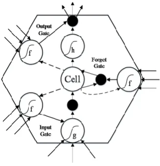
variant using the Depth gate [38], it is different from LSTM that it also decides what to forget and what new information to add. Another novel modified variant is the Gated Recurrent Unit (GRU) proposed by Cho, et al. in 2014 [39], which combined the forget gate and input gate to a single update gate. The specific structure of the LSTM model is shown in Figure 1 :
Figure 1.Structure of the LSTM neural network
state in the previous time step. Three weights are brought into the input node, forget gate, and output gate respectively. The activation function (S-type function) is connected to a black node, and the internal state of the unit is the most central node. The weight across the time step is set to 1, while the self-feedback is made, and the constant error conveyor (CEC) is the connection edge of the internal state. In the model, if the input sequence is set to(x1,x2, . . . ,xT)and the state of the hidden layer is set
to(h1,h2, . . . ,hT), then at timet, there are:
it=sigmoid(Whiht−1+WxiXt) (1) ft=sigmoid(Wh fht−1+Wx fXt) (2) ot=sigmoid(Whoht−1+WhxXt+Wcoct) (3) ct= ftct−1+ittanh(Whcht−1+WxcXt) (4)
ht=ottanh(ct) (5)
In the formula above, it represents input gate, ftrepresents forget gate,otrepresents output gate, ctrepresents cell,Whrepresents the weight of recursive link,Wxrepresents the weight from the output
layer to the hidden layer, the activation functions aresigmoidand tanh.
As can be seen from the above figure and formula, LSTM neural network is a special RNN, it can learn from the information of a long-term to solve the problem of gradient disappearance by increasing the memory unit. Therefore, this paper applied it to the hourly traffic flow forecast of the middle and long-term period for the first time.
2.2. LSTM Neural Network Based on Self-adaptive Probabilities
The LSTM neural network has the function of preventing the gradient disappearance and
long-term memory, but it also has the problem of over-fitting [40]. The so-called over-fitting
phenomenon is that the trained model has a good performance on the training data set, but its
performance on the test set is poor [41]. The causes of this phenomenon include excessive noise
interference, high model complexity and so on. In this paper, the situation that the LSTM neural network is applied to the traffic flow prediction, making the noise interference an important incentive for the over-fitting phenomenon.
To solve the over-fitting problem, Hinton proposed a solution that uses Dropout in 2014 [42].
Dropout refers to discard the neural network unit from the network temporarily according to a certain probability during the training process of the depth learning network. That is, Dropout randomly selects a part of the neurons, then sets its output as 0, and remains its previous values at the same time, and restores the previous retention value in the next training process, and then randomly selects, and repeats this process. In this way, the network structure changes in each training process, so as to avoid the situation that a feature is effective only with the support of the specific characteristics of other features, thus reducing the probability of over-fitting in the training process.
Although Hinton, et al. proposed Dropout to reduce the probability of over-fitting, but they do not go into the calculation method seriously of the key parameter involved in Dropout - the probability of selective discarding neurons, while they use the empirical value of 0.5. The reason is that the network structure generated randomly is the most in this case. In recent years, the empirical value is also used in the related applications based on LSTM. In order to solve this problem, this paper made a study and proposed the method of calculating the probability value of selective discarding neurons in Dropout to improve the self-adaptive over-fitting of LSTM neural network.
local feature optimal solution when the noise is too small. Therefore, the proportion of singular points has an important impact on the training results. And the probability value of selectively discarding neurons in Dropout also expresses the proportion of the screening of data to a certain extent. Therefore, there is a large degree of critical link between the two. At the same time, it was found in this paper that if we use the time singularity ratio as the probability value of selectively discarding neurons in Dropout, we can guarantee that the singular points are not discarded totally and they exist to a certain degree. The reason is as follows:
Nd Nj
= Nq
N (6)
Nj =Nd+Nu (7)
It can be deduced formula (6), (7) that:
Nqd Nj
≤ Nd
Nj
(8)
In the formula above,Ndrepresents the number of discarded nodes,Njrepresents the number
of nodes of each layer,Nqrepresents the number of singular points,Nrepresents the number of all
nodes in the single-layer network,Nurepresents the number of nodes that is not discarded in the
single-layer network,Nqdrepresents the number of nodes in the single-layer network that are both
discarded and belong to noise. It can be seen that the improved method proposed in this paper can make the probability of selecting the node needed to delete randomly in Dropout more reasonable, and its effect to prevent over-fitting problem is more prominent.
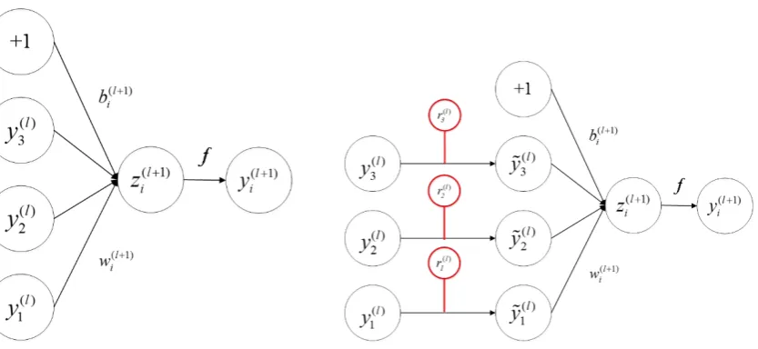
We call the improved neural network adaptive to prevent over-fitting LSTM neural network: Singular Point Probability LSTM (SDLSTM). The SDLSTM are shown as follows:
Formula expressions are as shown below, the unimproved formulas are as follows:
Zi(l+1)=wi(l+1)yl+b(il+1),
y(il+1)= f(z(il+1)).
(9)
The formulas of Adaptive to prevent over-fitting LSTM neural network are as follows:
p= Nq
N,
r(jl)∼Bernoulli(p), ˜
yi(l)=rj(l)×y(l),
zi(l+1)=w(il+1)y˜(il)+b(il+1),
y(il+1)= f(z(il+1)).
(10)
In Figure 2 and (9), (10),z(il+1)represents the value of thei-th neuron of thel+1-th layer,w(il+1)
represents the weight of thei-th connection of thel+1-th layer,bi(l+1)represents the bias of thei-th neuron of thel+1-th layer, yi(l+1) represents the output of thei-th neuron of the l+1-th layer, f
(a) Standard neural network layer (b) Improved neural network layer
Figure 2.Network layer
2.3. Traffic Data Flow Time Singularity Ratio Definition and Algorithm
To obtain the value of the time singularity ratio of the traffic flow proposed in this paper, it is necessary to obtain the number of singular points and the number of all the sample points, where the latter is known. Therefore, we only need to calculate the number of singular points. And for the
detection methods of singular point, domestic and foreign scholars have been studied [43], but in
this paper, we need to carry out the detection of singular point in traffic flow. In view of the high temporality of traffic flow, a method of self-adaptive singular point detection using time series is
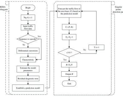
proposed. The flow chart of the algorithm is shown in Figure 3. . In the figure above,Nqrepresents
the number of singular points,tis the sequence of time periods in the traffic flow data,Ctrepresents
the difference between the traffic flow predicted during the time period and the actual traffic flow,Pt
represents the traffic flow predicted during the time period,Rtrepresents the actual traffic flow during
the time period,Ntrepresents the number of time periods in the data set,Nrepresents the number of
all data in the data set, andBis the required singularity ratio.
As shown in Figure 3. The method of determining the time singularity ratio of the traffic data flow is mainly composed of two parts. One part is the establishment of the ARIMA model, and the steps are the same as that of the general ARIMA model, which include the smoothness detection, differential transformation, feature analysis, parameter estimation, etc. [44].
The other part is the singular point detection part of the self-adaptive traffic flow. In this part, based on the ARIMA prediction model obtained in the previous section and the previous data, the data of the next time period are predicted successively to obtainPt, and then we calculated the differenceCt
ofPtand the actual traffic flowRtof the time period. When the difference is obtained, it is compared
with the threshold to determine whether the data belongs to the singular point. For the selection of thresholds, this paper considered that the order of magnitude of traffic flow is different at different time intervals, so it is unreasonable to set constant threshold, which will lead to big error of the result of singular point detection. Thus, this paper used 10% of the average of the traffic flow over a period of time in the data set as the threshold of the singular point detection in the time period, so that the threshold is changing over the time period, the traffic flow data is self-adaptive in different time periods and the accuracy of singular point detection is much higher. After the threshold comparison is
made, the number of singular points can be counted and then divided by the numberNof all data
ARIMA modeling part
Singular points detection part Begin
Nq=0, t=1
Input traffic flow data
Sequence is smooth?
Differential conversion
Characteristic
Estimate the model parameters
Residual diagnostic tests
Establish a prediction model
Forecast the traffic flow of the next hour (Pt) based on
the prediction model
Ct=|Pt-Rt|
Nq=Nq+1
t N ?
B=Nq/N
Output B
End Yes
Yes No
No
T=t+1
Figure 3.Flowchart of singular ratio determination method in improved LSTM neural network
3. Improved Forecasting Models Using SDLSTM and ARIMA
This work found that the MAPE value of SDLSTM prediction method is high in 6 o’clock. By analyzing experimental data,the main reason led to high MAPE in 6 o’clock is that the traffic flow changed severely during this period. The complicated features and high real time meant that LSTM cannot learn the whole features of this time slot. Thus, the prediction using deep learning method is not suit for this time slot. Meanwhile, ARIMA algorithm does not demand too much on data volume,
and it has high real time and low algorithm complexity [45]. In result, this paper aimed at solving
the non-ideal result of 6 o’clock predication by bringing in traffic flow prediction method based on ARIMA. ARIMA doesn’t have the training process of data learning, so it is much suit for shorter period prediction. And the result is not ideal in the medium and long-term prediction. Aiming at this problem, this paper solved it by combining LSTM and ARIMA with non-equal interval, that is the non-equal interval traffic flow prediction method based on SDLSTM neural network and ARIMA (a.k.a. SDLSTM-ARIMA).
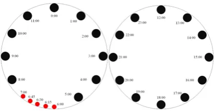
Non-equal interval, that is, in the prediction period of LSTM, regarding 1 hour as unit time; in prediction period of ARIMA, regarding 15 min as unit time. Under this circumstance, the traffic flow prediction in different periods during one day forms the condition of the combination of non-equal intervals, as shown in Figure 4.
In the figure 4, the prediction in 6 o’clock used 15 min as a circle (red dot), the prediction of other time slots regarded 1 hour as a circle (black dot). Then, by the mode of non-equal interval combination, we combined the advantages of LSTM and ARIMA models together to improve the real time and accuracy of the traffic flow prediction.
Figure 4.SDLSTM-ARIMA non-equal interval combination diagram
Traffic flow data Dn
Dn
SDLSTM
ARIMA
Judge and output
SDLSTM netural networks training
Dropout
parameter
Dn
SDLSTM netural networks training
Pn+1
Pn+1
SDLSTM
ARIMA
Traffic flow data
Pn+1
Judge and output
Traffic flow data
SDLSTM
ARIMA
SDLSTM netural networks training
Dn-1
Dn-1
Dn-1
Judge and output
Pn
Pn
Dropout
parameter
Dn+1
Dn+1
Dn+1
…
…
Tn-1 Tn Tn+1
Dropout
parameter
Figure 5.Cluster computing model of the traffic prediction method of this work
4. Cluster Computing Model
4.1. Cluster computing model of SDLSTM-ARIMA
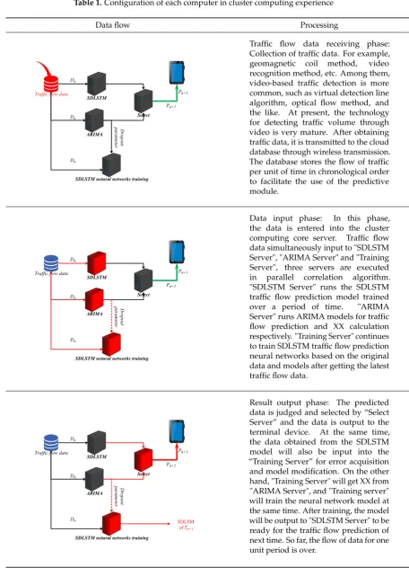
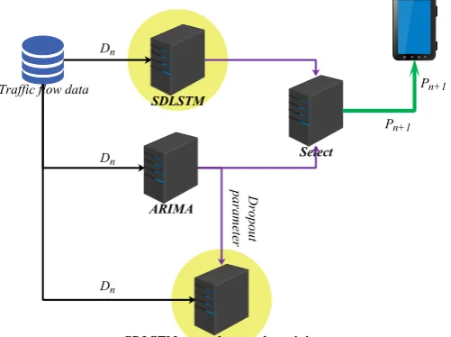
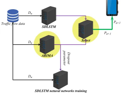
As illustrated in Figure 5, this work realized the algorithm by cluster computing. The servers with a yellow background combined a cluster in cycle time. There are “SDLSTM server”, “ARIMA server”, “Training server” and “Select server”. In the cluster, the “SDLSTM server” runs the computing programs of SDLSTM training from “Training server” in the Tn-1 period. The “SDLSTM server” output the prediction result of the next time by using SDLSTM method. The “ARIMA server” runs the computing programs of ARIMA. This server will get the prediction result of the next time by using ARIMA and the parameter of Dropout: time singularity ratio. The “Training server” runs the programs of training SDLSTM models. This server gets the prediction traffic flow in Tn by using SDLSTM method from the “SDLSTM server”, the real traffic flow in Tn from Database and the parameter of Dropout: time singularity ratio from the “ARIMA server”. And then, the “Training server” runs the programs of training SDLSTM neural networks. It will output the training results to the “SDLSTM server” to predict the traffic flow of next time and save to local to prepare the next time training. The “Select server” gets the prediction results by using ARIMA and the prediction results by using SDLSTM, the server will select which result to output. Data are input in parallel, and three servers run at the same time to achieve cluster computing effect and save computing time.
4.2. Data flow of the Cluster computing model
Table 1.Configuration of each computer in cluster computing experience
Data flow Processing
Traffic flow data Dn
Dn
SDLSTM
ARIMA
Select
SDLSTM netural networks training
Dropout
parameter
Dn
Pn+1 Pn+1
Traffic flow data receiving phase: Collection of traffic data. For example, geomagnetic coil method, video recognition method, etc. Among them, video-based traffic detection is more common, such as virtual detection line algorithm, optical flow method, and the like. At present, the technology for detecting traffic volume through video is very mature. After obtaining traffic data, it is transmitted to the cloud database through wireless transmission. The database stores the flow of traffic per unit of time in chronological order to facilitate the use of the predictive module.
Traffic flow data Dn
Dn
SDLSTM
ARIMA
Select
SDLSTM netural networks training
Dropout
parameter
Dn
Pn+1 Pn+1
Data input phase: In this phase, the data is entered into the cluster computing core server. Traffic flow data simultaneously input to "SDLSTM Server", "ARIMA Server" and "Training Server", three servers are executed in parallel correlation algorithm. "SDLSTM Server" runs the SDLSTM traffic flow prediction model trained over a period of time. "ARIMA Server" runs ARIMA models for traffic flow prediction and XX calculation respectively. "Training Server" continues to train SDLSTM traffic flow prediction neural networks based on the original data and models after getting the latest traffic flow data.
Traffic flow data Dn
Dn
SDLSTM
ARIMA
Select
SDLSTM netural networks training
Dropout parameter Dn Pn+1 Pn+1 SDLSM of Tn+1
executes related algorithms through the monitoring end computing device or the cloud computing device, and statistically obtains the traffic flow and saves it in the database. The data input part is to input traffic flow data obtained in parallel to "SDLSTM Server", "ARIMA Server", "Trainning Server". The output part consists of two branches. One is to forward the prediction data of “SDLSTM Server” and “ARIMA Server” to “Select Server” and output the final prediction result. The other is to input the training result of “Training Server” to “ "SDLSTM Server" to prepare for the prediction of the next period of time.
5. Performance Evaluation
5.1. Experimental Setup
Figure 6.The location of the monitoring point
The experimental data in this paper comes from the traffic flow data set published publicly in the official website of British Columbia of Canada [46], and the experiment is based on the data from Vancouver Richmond region. The road condition at the monitoring point are shown in Figure 6. During the process of the experiment, a total of 43824 hours of data (from January 1, 1999 to December 31, 2003) of the monitoring point are used, with data of May 21, 2003 and after as test data and data before that date as training data. The total test data has 5400 hours and the total training data has 38424 hours.
Firstly, this paper took a week as a cycle and number of weeks as label, and extracted traffic flow in the data by day. As shown form Figure 7(a). To Figure 7(g). The abscissa is time and the ordinate is traffic flow. It can be seen from the figures that the number of different days in a week has a relatively fixed trend, which further proves the feasibility of using the model obtained by LSTM training.
Thus, this model can be used to model the different days of a week based on the trend. Through a large number of data training, we added the characteristics of a week to the model, so that the training model can adapt to the changing trend each week during the four years, and the law of the four years also has enough universality. The forecasting model obtained by four years’ traffic flow data training is more consistent with long historical trends, and a lower error rate is guaranteed in this dimension. In the training process, we increased the training input vector to 24 hours, and regarded the output of the forecast data as the traffic flow for the next hour. By using the method of deep learning, the characteristics of traffic flow information are excavated, and 24 hours’ traffic flow is entered in real time. This paper took the factors of real-time traffic flow and historical traffic flow into account, ensured real-time and improved accuracy at the same time.
(a) Sunday (b) Monday
(c) Tuesday (d) Wednesday
(e) Thursday (f) Friday
(g) Saturday
Table 2.Configuration of each computer in cluster computing experience
Servers Computer configuration
ARIMA Server 2-core, per 2.5GHz, 8G SDLSTM Server 2 Core, per 2.5GHz, 8G Training Server 4 Core, per 2.5GHz, 32G Select Server 2 Core, per 2.5GHz, 8G
5.2. Results of the Proposed SDLSTM-ARIMA Method
As illustrated in Figure 8, the SDLSTM server runs the SDLSTM natural networks training from Training server to predict traffic flow of next time. One of the error changes in the training process is shown in Figure 9.
Traffic flow data Dn
Dn
SDLSTM
ARIMA
Select
SDLSTM netural networks training
Dropout
parameter
Dn
Pn+1
Pn+1
Figure 8.Servers about SDLSTM
Figure 9.The change of MAPE with epoch during training
The formula shows the method of calculating the MAPE value of the data deviation. As shown in
Figure 9. The MAPE value [47] is changing during the training process of LSTM by the data training
the MAPE value tends to be stable after the epoch value reaches 40. It shows that the number of the training done to sample set in this paper is enough sufficient.
MAPE=
∑
X−Y X N
!
×100%÷N (11)
2 4 6 8 10 12 14 16 18 20 22 24
0 2 4 6 8 10 12 14 16 18
Samling T ime
M
AP
E
Monday T uesday Wednesday T hursday Friday Saturday Sunday
Figure 10.The change of MAPE with epoch during training
As can be seen from the above Figure 10, the six o’clock prediction error is large. In this regard, we have made improvements. The SDLSTM-ARIMA traffic flow prediction algorithm is proposed. As shown in the Figure 11, the ARIMA-based traffic flow prediction program was added to the "ARIMA Server". Added "Select Server" to select data based on different time periods.
Traffic flow data Dn
Dn
SDLSTM
ARIMA
Select
SDLSTM netural networks training
Dropout
parameter
Dn
Pn+1 Pn+1
Figure 11.The change of MAPE with epoch during training
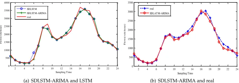
The improved LSTM neural network for data training is used in this paper, and the process of MAPE changes are shown in Figure 9. Above. The ordinary LATM neural network method obtained by training is compared with the SDLSTM-ARIMA method proposed in this paper, as shown in Figure 12(a)., where the red part of the figure shows the improvement of the accuracy of the prediction after the introduction of the ARIMA model, and the result of the comparison proved the effectiveness of SDLSTM-ARIMA.
2 4 6 8 10 12 14 16 18 20 22 24 0 500 1000 1500 2000 2500 3000 3500 4000
Sampling T ime
F lo ws (v e h /h o u r) SDLST M SDLST M-ARIMA real
(a) SDLSTM-ARIMA and LSTM
2 4 6 8 10 12 14 16 18 20 22 24
0 500 1000 1500 2000 2500 3000 3500
Sampling T ime
F lo ws (v e h /h o u r) real SDLAT M-ARIMA
(b) SDLSTM-ARIMA and real
Figure 12.Comparison of predicted values
forecast value and the actual value of one month of the results; as can be seen from the graph, in the LATM-AR experimental test results, the predicted traffic flow data is basically consistent with the actual data and the method has high accuracy.
20 40 60 80 100 120 140 160 180 0 500 1000 1500 2000 2500 3000 3500 4000
Sampling T ime
F lo ws (v eh /h o u r) SDLST M-ARIMA real
Figure 13.The predicted values obtained by SDLSTM-AR method compared with the real values in a week
100 200 300 400 500 600 700
0 500 1000 1500 2000 2500 3000 3500 4000
Sampling T ime
F lo ws (v eh /h o u r) SDLAT M-ARIMA real
Figure 14.The predicted values obtained by SDLSTM-AR method compared with the real values in a month
5.3. Comparative Results of different kinds of traffic flow forecast methods
Using the training data set and the test data set, this paper compared the commonly used
ARIMA prediction method and the latest proposed AR-RBLTFa method in reference [17] with the
working days, Figure 15(b). Shows the comparison of the data of Non-working days. As can be seen from the figure, compared with the commonly used ARIMA prediction method, AR-RBLTFa method and SDLSTM-ARIMA have higher accuracy.
2 4 6 8 10 12 14 16 18 20 22 24 0 500 1000 1500 2000 2500 3000 3500 4000
Sampling T ime
Fl o w s (v e h /h o u r) ARIMA AR+RBLT Fa SDLST M-ARIMA real
(a) Working days
2 4 6 8 10 12 14 16 18 20 22 24 0 500 1000 1500 2000 2500
Sampling T ime
F lo ws (v eh /h o u r) ARIMA AR+RBLT Fa SDLST M+ARIMA real
(b) Non-working days
2 4 6 8 10 12 14 16 18 20 22 24 0 20 40 60 80 100 120 140 160 180 200
Samping T ime
F lo ws (v e h /h o u r) ARIMA AR+RBLT Fa SDLST M+ARIMA
(c) MAPE values of workday
2 4 6 8 10 12 14 16 18 20 22 24 0 200 400 600 800 1000 1200
Sampling T ime
F lo ws (v e h /h o u r) ARIMA AR+RBLT Fa SDLST M+ARIMA
(d) MAPE values of non-workday
2 4 6 8 10 12 14 16 18 20 22 24 -1500 -1000 -500 0 500 1000 1500
Sampling T ime
F lo ws (v e h /h o u r) ARIMA AR+RBLT Fa SDLST M-ARIMA
(e) Absolute errors of workday
2 4 6 8 10 12 14 16 18 20 22 24 -800 -600 -400 -200 0 200 400 600 800
Sampling T ime
Fl o w s (v e h /h o u r) ARIMA AR+RBLT Fa SDLST M-ARIMA
(f) Absolute errors of non-workday
2 4 6 8 10 12 14 16 18 20 22 24 0 200 400 600 800 1000 1200 1400
Sampling T ime
F lo ws (v eh /h o u r) ARIMA AR+RBLT Fa SDLST M-ARIMA
(g) RMSE of Workday
2 4 6 8 10 12 14 16 18 20 22 24 0 200 400 600 800 1000 1200
Sampling T ime
F lo ws (v eh /h o u r) ARIMA AR+RBLT Fa SDLST M-ARIMA
(h) RMSE of non-workday
Figure 15.Comparison of experimental results of different methods
After obtaining the traffic flow data of the three methods, in order to measure the error of the three methods much better, the MAPE value and the absolute error of the three methods are calculated and compared in this paper. Figure 15(c). shows the comparison of MAPE values of working days of the three methods; Figure 15(d). shows the comparison of MAPE values of non-working days of the three methods; Figure 15(e). shows the comparison of the absolute error of working days of the three methods; Figure 15(f). shows the comparison of the absolute errors of non-working days of the three methods; Figure 15(g). shows the comparison of RMSE values of working days of the three methods; Figure 15(h). shows the comparison of RMSE values of non-working days of the three methods; And RMSE calculation method is as shown in the Formula (12):
RMSE=
s
∑n
i=1(xreal−xpre)
n (12)
In the formula above,nrepresents the number of time points,xrealrepresents the real traffic flow at the
time point, andxprerepresents the predicted traffic flow at the time point.
compared, as shown in Table 3. As can be seen from the table, the accuracy rate is: SDLSTM-ARIMA
>AR-RBLTFa>ARIMA, while the error stability is: SDLSTM-ARIMA>AR-RBLTFa>ARIMA.
Therefore, the
SDLSTM-ARIMA proposed in this paper has higher accuracy and stability.This work also improved the SDLSTM-ARIMA by cluster computing. As shown in Table 4, the running time is much reduced by cluster computing.At last, this paper summarized the advantages and disadvantages of the three methods, as shown in Table 5.
Table 3.Quantitative comparison of three methods
Evaluating Indicator ARIMA AR-RBLTFa SDLSTM-ARIMA
MPAE 40.43 14.46 10.26
RMSE 611.4 184.49 176.90
Absolute Error 498.59 156.41 138.25
Error Entropy (normalized) 1 0.24 0.09
Table 4.Running time comparison of three prediction methods
Algorithm Time
ARIMA 0.201s
AR-RBLTFa 0.784s
SDLSTM-ARIMA 4.124s
SDLSTM-ARIMA by cluster computing 0.799s
Table 5.Comparison of three prediction methods
Algorithm Accuracy Dependence on
historical data
Stability of forecast data
Real-time of the prediction
ARIMA general slight low Low Predict on time
AR-RBLTFa high high General Predict on time
SDLSTM-ARIMA slight high slight high High Delay in variable scale adjustment SDLSTM-ARIMA by
cluster computing slight high slight high High Predict on time
6. Conclusions
Author Contributions:Conceptualization, Boyi Liu; Data curation, Xiangyan Tang; Formal analysis, Boyi Liu; Funding acquisition, Jieren Cheng; Methodology, Boyi Liu; Project administration, Jieren Cheng; Resources, Jieren Cheng; Writing – original draft, Boyi Liu; Writing – review and editing, Qiang Liu.
Funding: This research was funded by [National Natural Science Foundation of China] grant number [61363071, 61762033, 61379145, 61702539], [The National Natural Science Foundation of Hainan] grant number [617048],[Hainan University Doctor Start Fund Project] grant number [kyqd1328],[Hainan University Youth Fund Project] grant number[qnjj1444].[National innovation and entrepreneurship training program for College Students],grant number[201610589022, 201610589002]
Acknowledgments:Thanks for the participants of NCTCS 2017,they provided many useful suggestions for the algorithm and its feasibility.
Conflicts of Interest:The authors declare no conflict of interest.The founding sponsors had no role in the design of the study; in the collection, analyses, or interpretation of data; in the writing of the manuscript, and in the decision to publish the results.
References
1. Hu X, Chu T H S, Chan H C B, et al. Vita: A Crowdsensing-Oriented Mobile Cyber-Physical System.IEEE Transactions on Emerging Topics in Computing2013,1(1), 148-165.
2. Hu X, Li X, Ngai E, et al. Multidimensional context-aware social network architecture for mobile crowdsensing.IEEE Communications Magazine2014,52(6), 78-87.
3. Alam M, Ferreira J, Fonseca J. Introduction to intelligent transportation systems[C]//Intelligent Transportation Systems. Springer International Publishing, 2016: 1-17.
4. Moral-Muñoz J A, Cobo M J, Chiclana F, et al. Analyzing highly cited papers in Intelligent Transportation Systems [J]. IEEE Transactions on Intelligent Transportation Systems, 2016, 17(4): 993-1001.
5. Bright P W, Balmforth Z, MacPherson J L. The effect of changes in traffic flow on mammal road kill counts[J]. Applied Ecology and Environmental Research, 2015, 13: 171-179.
6. Habtemichael F G, Cetin M. Short-term traffic flow rate forecasting based on identifying similar traffic patterns[J]. Transportation Research Part C: Emerging Technologies, 2016, 66: 61-78.
7. Lv Y, Duan Y, Kang W, et al. Traffic flow prediction with big data: a deep learning approach[J]. IEEE Transactions on Intelligent Transportation Systems, 2015, 16(2): 865-873.
8. Hou Y, Edara P, Sun C. Traffic Flow Forecasting for Urban Work Zones[J]. IEEE Transactions on Intelligent Transportation Systems, 2015, 16(4): 1761-1770.
9. Romero D, Rico N, Garcia-Arenas M I. Modellation and Forecast of Traffic Series by a Stochastic Process[M]//Time Series Analysis and Forecasting. Springer International Publishing, 2016: 279-292. 10. Lopez-Garcia P, Onieva E, Osaba E, et al. A hybrid method for short-term traffic congestion forecasting
using genetic algorithms and cross entropy[J]. IEEE Transactions on Intelligent Transportation Systems, 2016, 17(2): 557-569.
11. Fan Na, Zhao Xiangmo, Dai Ming, et al. Short-term traffic flow prediction model[J]. Journal of Traffic and Transportation Engineering, 2012,04:114-119.
12. Kumar S V, Vanajakshi L. Short-term traffic flow prediction using seasonal ARIMA model with limited input data[J]. European Transport Research Review, 2015, 7(3): 1-9.
13. Moorthy C K, Ratcliffe B G. Short term traffic forecasting using time series methods[J]. Transportation planning and technology, 1988, 12(1): 45-56.
14. Williams B, Durvasula P, Brown D. Urban freeway traffic flow prediction: application of seasonal autoregressive integrated moving average and exponential smoothing models[J]. Transportation Research Record: Journal of the Transportation Research Board, 1998 (1644): 132-141.
15. Stephanedes Y J, Michalopoulos P G, Plum R A. Improved estimation of traffic flow for Real-Time control (Discussion and closure)[J]. Transportation Research Record, 1981 (795).
16. Okutani I, Stephanedes Y J. Dynamic prediction of traffic volume through Kalman filtering theory[J]. Transportation Research Part B: Methodological, 1984, 18(1): 1-11.
17. Misra C, Fan Y, Davatzikos C. Baseline and longitudinal patterns of brain atrophy in MCI patients, and their use in prediction of short-term conversion to AD: results from ADNI[J]. Neuroimage, 2009, 44(4): 1415-1422. 18. Teles J, Pina C, Edén P, et al. Transcriptional regulation of lineage commitment-a stochastic model of cell fate
19. Hou Z, Li X. Repeatability and Similarity of Freeway Traffic Flow and Long-Term Prediction Under Big Data[J]. IEEE Transactions on Intelligent Transportation Systems, 2016, 17(6): 1786-1796.
20. Davis G A, Nihan N L. Nonparametric regression and short-term freeway traffic forecasting[J]. Journal of Transportation Engineering, 1991, 117(2): 178-188.
21. Dougherty M. A review of neural networks applied to transport[J]. Transportation Research Part C: Emerging Technologies, 1995, 3(4): 247-260.
22. Xu Yanyan, Zhaixi, Kong Xiqing, et al. Short-term prediction method of freeway traffic flow[J]. Journal of Traffic and Transportation Engineering, 2013,02:114-119.
23. Liu F, Liu B, Sun C, et al. Deep belief network-based approaches for link prediction in signed social networks[J]. Entropy, 2015, 17(4): 2140-2169.
24. Bai C, Peng Z R, Lu Q C, et al. Dynamic bus travel time prediction models on road with multiple bus routes[J]. Computational intelligence and neuroscience, 2015, 2015: 63.
25. Yanchong C, Darong H, Ling Z. A short-term traffic flow prediction method based on wavelet analysis and neural network[C]//Control and Decision Conference (CCDC), 2016 Chinese. IEEE, 2016: 7030-1034. 26. Moretti F, Pizzuti S, Panzieri S, et al. Urban traffic flow forecasting through statistical and neural network
bagging ensemble hybrid modeling[J]. Neurocomputing, 2015, 167: 3-7.
27. Tian Y, Pan L. Predicting Short-Term Traffic Flow by Long Short-Term Memory Recurrent Neural Network[C]//2015 IEEE International Conference on Smart City/SocialCom/SustainCom (SmartCity). IEEE, 2015: 153-158.
28. Butt M. Selection of forecast model for consumption (four sectors) and transmission (two Piplines) of natural gas in Punjab (Pakistan) based on ARIMA model[J]. International Journal of Advanced Statistics and Probability, 2015, 3(1): 115-125.
29. Boyi Liu, Jieren Cheng, Kuanqi Cai. Singular Point Probability Improve LSTM Network Performance for Long-term Traffic Flow Prediction[C]//35th National Conference on Theoretical Computer Science. 2017:328-340..
30. Zhu X, Sobhani P, Guo H. Long short-term memory over recursive structures[C]//Proceedings of the 32nd International Conference on Machine Learning. 2015: 1604-1612.
31. Rakkiyappan R, Chandrasekar A, Cao J. Passivity and passification of memristor-based recurrent neural networks with additive time-varying delays[J]. IEEE transactions on neural networks and learning systems, 2015, 26(9): 2043-2057.
32. Luko˘sEvi˘cIus M, Jaeger H. Reservoir computing approaches to recurrent neural network training[J]. Computer Science Review, 2009, 3(3): 127-149.
33. Bahdanau D, Cho K, Bengio Y. Neural machine translation by jointly learning to align and translate[J]. arXiv preprint arXiv:1409.0473, 2014.
34. Liang M, Hu X. Recurrent convolutional neural network for object recognition[C]//Proceedings of the IEEE Conference on Computer Vision and Pattern Recognition. 2015: 3367-3375.
35. Pascanu R, Mikolov T, Bengio Y. On the difficulty of training recurrent neural networks[J]. ICML (3), 2013, 28: 1310-1318.
36. Hochreiter S, Schmidhuber J. Long short-term memory[J]. Neural computation, 1997, 9(8): 1735-1780. 37. Gers F A, Schmidhuber J, Cummins F. Learning to forget: Continual prediction with LSTM[J]. Neural
computation, 2000, 12(10): 2451-2471.
38. Yao K, Cohn T, Vylomova K, et al. Depth-Gated Recurrent Neural Networks[J]. 2015.Chung J, Gulcehre C, Cho K H, et al. Empirical evaluation of gated recurrent neural networks on sequence modeling[J]. arXiv preprint arXiv:1412.3555, 2014.
39. Srivastava N, Hinton G E, Krizhevsky A, et al. Dropout: a simple way to prevent neural networks from overfitting[J]. Journal of Machine Learning Research, 2014, 15(1): 1929-1958.
40. Zaremba W, Sutskever I, Vinyals O. Recurrent neural network regularization[J]. arXiv preprint arXiv:1409.2329, 2014.
41. Bailey D H, Borwein J M, de Prado M L, et al. Pseudomathematics and financial charlatanism: The effects of backtest over fitting on out-of-sample performance[J]. Notices of the AMS, 2014, 61(5): 458-471.
43. Awad A I, Baba K. Singular point detection for efficient fingerprint classification[J]. International Journal of New Computer Architectures and their Applications (IJNCAA), 2012, 2(1): 1-7.
44. Wang W, Chau K, Xu D, et al. Improving forecasting accuracy of annual runoff time series using ARIMA based on EEMD decomposition[J]. Water Resources Management, 2015, 29(8): 2655-2675.
45. Pati J, Shukla K K. A comparison of ARIMA, neural network and a hybrid technique for Debian bug number prediction[C]//Computer and Communication Technology (ICCCT), 2014 International Conference on. IEEE, 2014: 47-53.
46. Traffic data program of British Columbia. Public Traffic Data[EB/OL]. http://www.th.gov.bc.ca/trafficData/legacy/TDP-97-03.html
47. Chen J, Wang Y, Gu C, et al. Enhancement of the mechanical properties of basalt fiber-wood-plastic composites via maleic anhydride grafted high-density polyethylene (MAPE) addition[J]. Materials, 2013, 6(6): 2483-2496.