A Comparative Study of Performances of Various
Classification Algorithms for Predicting Salary
Classes of Employees
Swapnajit Chakraborti
Doctoral Student (Fellow Programme in Management, Industry), Information Systems, Indian Institute of Management Indore
Indore, M.P., India
Abstract— In knowledge based industry, compensation
planning is a key strategic area for growth and success. In order to retain high performance employees, optimum salary offer is essential. Determining such salary figures, based on various information about a current employee or a prospective employee, is a challenge that corporations face very frequently. Although HR managers typically tackle such salary prediction and negotiation issues in consultation with relevant department-level managers, any automated system with such capability would be of great help for them. Given the attributes of an employee (current or prospective), which includes her demographic profile along with other information such as qualification, performance level etc. , several well-known classification algorithms can be used for the prediction of the salary class. But unfortunately, such details of employee data of any corporation are generally not available in public for performance evaluation of classification algorithms. In this paper, this limitation is overcome to some extent by using a public database (UCI census dataset) which have most of the attributes available for a segment of population for salary prediction. Although the data used in this experimental paper is not directly related to salary prediction of employees within an organization, but it can be extrapolated to be used in the former scenario as the tuples in UCI census dataset include employer type as an attribute. This analysis found that among five classification algorithms, decision tree and Bayesian belief network performs better than other three algorithms, namely, naïve Bayes, support vector machine and neural network. The software used for running these algorithms is WEKA which is a well-known university tool for machine learning.
Keywords
—
Human Capital, Human Resource,Compensation Management, Salary Prediction, Knowledge Based Industry, Classification Algorithms, Machine Learning, Naïve-Bayes, Bayesian Belief Network, Support Vector Machine, SVM, Decision Tree, Neural Network, Back-propagation
I. INTRODUCTION
With more and more focus on knowledge based industry, the compensation planning for the human capital is becoming a key strategic area for companies to ensure sustained growth and success. One of the problems which corporations face today is the challenge of retaining high-performing employees and also hire talented people from other organizations. In both the cases, salary happens to be a key decisive factor for enticing current as well as prospective employees. Hence an optimal salary offer,
which is win-win for both the employee (current as well as prospective) and the company, is extremely important for retaining or attracting employees to any organization. Human resource managers have long realized that many factors affect the salary expectation of an employee and only her past performance or performance during interview is not the sole determiner of her expected salary. Hence recruiters need to weigh various factors including demographic as well as others to make final offer to an employee. Although experienced human resource managers drive this exercise in consultation with the relevant department level manager, it is always a difficult decision. Any kind of automated decision making system would be of extreme help for these decision makers to come up with appropriate salary recommendations. In general, companies do have their compensation prediction system which utilize internal data for predicting salary of a new hire. But such data is not available for external usage and hence any analysis of such predictive system need to use externally available data. In this research paper, a public data set available from University of California, Irvine (UCI) repository is used for experimenting with various machine learning algorithms for prediction of salary and also measure their comparative performances. Although the data used in this experimental paper is not directly related to salary prediction of employees within an organization, but it can be extrapolated to be used in the former scenario as this also deals with binary salary class prediction of a segment of population who work for multiple organizations. In real company scenario, the salary classes may be more than two and the population will be from within a single company and hence from that angle, this binary modelling is also not one-to-one mapping of the real scenario. Despite this fact, the classification experiment undertaken in this research paper using multiple machine learning algorithms on the UCI census dataset (University of California, 1994), can definitely be considered as a useful effort towards understanding the effectiveness of these algorithms for real salary prediction problem. Although there are multiple limitations, yet the findings can be used in actual problem settings.
days, classification has become an integral part of decision making process within many organizations. Classification is a two-step process, consisting of a learning step and classification step. The former creates the classification model using the training tuples while the latter uses the model to do the prediction of appropriate label/class for test tuples. Typically, the learning phase of a classifier uses training tuples which are labelled a priori. Hence classification is considered as a form of supervised learning method. There are several well-known classification techniques, namely, decision trees, naïve-Bayes, Bayesian belief network, support vector machine, back propagation neural network, rule-based systems etc.
As mentioned earlier, this paper explores the comparative performance of some of these standard classification algorithms on a well-known dataset, namely census dataset available from UCI. The basic purpose is to develop clear understanding about the applicability of these algorithms for salary prediction of employees (current or prospective) of an organization and their comparative performance figures.
II. RELATED WORK
The census dataset from UCI (University of California, 1994) has been used in multiple cases (University of California, 1994) but none with the intent of using it for employee salary prediction. In fact, no work is published which evaluates performance figures of various machine learning algorithms for salary classification problem. Although some work is available for predicting employee churn, no significant work is found on application of machine learning for employee salary classification.
III.DATASET AND PROBLEM STATEMENT
The census dataset from UCI (University of California, 1994) contains fifteen demographic attributes/features for each member of a population of size 32,561 including their individual salary class. The dataset is not specific to any company and that is why it doesn’t contain any performance attribute. There are two possible salary classes for a person, namely, greater than US$ 50K (>50K) and less than or equal to US$ 50K (<=50K). This dataset is not balanced in terms of the numbers of these two salary classes as approximately 30% of the tuples in the dataset belong to >50K class and rest 70% tuples belong to <=50K category. The dataset contains data primarily for male workers (21,790) of private companies who belong to white category (27,816). In terms of education levels, the dataset represents all kinds of categories, namely, bachelors, HS, masters, doctorate etc.
The basic problem is to find out a classification algorithm which will result in maximum accuracy in prediction of salary class (>50K, <=50K) based on the given set (or subset) of attributes. Hence the objectives of this paper are the following:
Run various classification engines on the UCI census dataset
Compare prediction performance of various classification engines in terms of precision, recall,
true positive rate (TP Rate), false positive rate (FP Rate), F-measure and area under ROC curve
Assess impact of feature selection techniques on quality of results and find out if a subset of features can be sufficient for training instead of the full set for achieving optimal performance.
Compare the training time (model build time) of the classification engines
This research experiment uses the well-known WEKA (Waikato, n.d.) machine learning software to run various classification engines on the UCI census dataset. The experiments are performed using a Windows 7, Intel i7 CPU @1.9 GHz, 8 GB RAM machine.
It should be noted that investigation of the impact of feature selection is included as one of the objectives, because many a time proper choice of a subset of feature improves prediction performance as well as training time of the classification algorithms. Especially in cases where number of features is huge, it is essential to filter out a manageable but effective subset of features to train the classification algorithms. Although, in this case, the number of features is very small, the feature selection experiment is also undertaken to explore and understand the impact on classification accuracy and performance. The wrapper method of feature selection available in WEKA is used in this case as it is suitable for machine learning.
It should be noted that the basic intention of this research is to carry out a comparative analysis of salary classification algorithms so that this knowledge can be used in real-life salary prediction by the companies. As discussed earlier, these findings will provide significant insight into the effectiveness and applicability of these algorithms in case of actual employee data which, unlike the UCI set, will be specific to one company and will include many other attributes such as performance level etc.
There are other ways to compare classifiers without using the accuracy metrics and training time, e.g. runtime performance, scalability, interpretability, which are not being considered in this paper.
IV.EXPERIMENTAL RESULTS AND ANALYSIS
There are several algorithms for classification of which the most well-known and widely applicable ones are run on the given dataset. The results of each of these runs using WEKA (Waikato, n.d.) are provided below. It should be noted that all results are based upon running the classification engines using all 15 attributes including the label class (salary class) which is the outcome. For cases where feature selection phase is run the number of features used for classification is mentioned explicitly.
A. Results for Naïve-Bayes Classification Algorithm
TABLEI
PREDICTIONPERFORMANCEMETRICSFORNAÏVE-BAYES
CLASSIFIER
Class
Performance Metrics
TP Rate
FP Rate
Precis
ion Recall F-Measu
re
ROC Area
>50K 0.517 0.065 0.716 0.517 0.6 0.892
<=50K 0.935 0.483 0.859 0.935 0.895 0.892
Wt.
Avg. 0.834 0.382 0.825 0.834 0.824 0.892
It is evident that the naïve-Bayes classifier model has better prediction performance for class <=50K compared to class >50K in terms of all metrics except ROC Area which is same for both. One possible reason for the classifier to predict <=50K class tuples more accurately, may be because of the unbalanced nature of the dataset which contains 70% tuples for class <=50K. Note that the ROC Area which is same for both classes, has value 0.892 which indicates excellent prediction accuracy. Some other relevant data as reported by WEKA are given in Table 2 below.
TABLE2
OTHERMETRICSFORNAÏVE-BAYESCLASSIFIER
The confusion matrix which is used for generating the prediction performance is given below in Table 3.
TABLE3
CONFUSIONMATRIXFORNAÏVE-BAYESCLASSIFIER
Class Classified As
>50K <=50K
>50K 4055 3786
<=50K 1610 23110
Typically, the prediction accuracy of any classifier is determined by the ROC curve and the area under ROC curve. The ROC curve for the two categories of salary classes, namely >50K and <=50K is shown below:
As already shown in Table 1 that area under ROC curve for both classes is 0.892 which is considered to be very good prediction performance for any classifier.
As mentioned earlier, one common practice in classification task is the selection of the best subset of features to be used for training the model. Although in this case, the number of features is not very large, feature selection experiment is performed using the exhaustive
search selection technique available in WEKA tuned for naïve-Bayes classifier. This will provide an optimal subset of features which can be used instead of the original set of features for obtaining maximum prediction performance.
The WEKA run selected the following 12 features out of 14 which form the subset for obtaining maximal performance: age, workclass, education, education-num, marital-status, occupation, relationship, race, sex,
capital-gain, hours-per-week and native-country. Hence feature selection process has excluded the two features, namely,
fnlwgt and capital-loss.
Although the size of the subset is not significantly less than original size of the feature set, it is found that when naïve-Bayes algorithm is re-run using this new subset of features, it results in better performance of the classifier. The new performance results of the classifier is shown in Table 4.
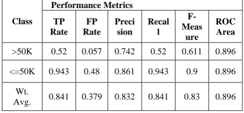
TABLE 4
PREDICTION METRICS FOR NAÏVE-BAYES CLASSIFIER WITH FEATURE SELECTION
Class
Performance Metrics
TP Rate
FP Rate
Preci sion
Recal l
F-Meas
ure
ROC Area
>50K 0.52 0.057 0.742 0.52 0.611 0.896
<=50K 0.943 0.48 0.861 0.943 0.9 0.896
Wt.
Avg. 0.841 0.379 0.832 0.841 0.83 0.896
The performance figures shows that feature selection step has resulted in better ROC Area for both classes as it reached 0.896 from 0.892. And the performance of classifier for both classes have improved marginally. Some other relevant data are given in Table 5 below.
Time taken to build model 0.15 seconds
Correctly classified instances 27165
(83.428%)
Incorrectly classified instances 5396
(16.572%)
Mean Absolute Error 0.1735
TABLE5
OTHERMETRICSFORNAÏVE-BAYESCLASSIFIERWITH
FEATURESELECTION
It is evident that training time performance or model build time of naïve-Bayes has improved by 80% and also the number/percentage of correctly classified instances has improved. Hence, in summary, feature selection has really boosted the overall performance of the classifier.
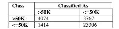
The confusion matrix which is used for generating the performance numbers is given below in Table 6.
TABLE6
CONFUSIONMATRIXFORNAÏVE-BAYESCLASSIFIERWITH
FEATURESELECTION
Class Classified As
>50K <=50K
>50K 4074 3767
<=50K 1414 23306
The ROC curve for both classes are same and is shown below:
As ROC Area is 0.896, the prediction accuracy is considered to be excellent.
B. Results for Decision Tree Classification Algorithm
The UCI dataset which has 14 attributes (nominal and numeric type) is extremely suited for applying decision tree based classifier. WEKA has the J48 decision tree classifier which implements C4.5 algorithm. For this experiment, it is run with 10-fold cross-validation on the UCI census dataset. Various metrics of its prediction accuracy and performance as reported by WEKA is provided below in Table 7.
TABLE7
PREDICTIONPERFORMANCEMETRICSFORDECISIONTREE(J48)
CLASSIFIER
Class
Performance Metrics
TP Rate
FP Rate
Preci sion
Recal l
F-Meas
ure
ROC Area
>50K 0.631 0.065 0.756 0.631 0.688 0.891
<=50K 0.935 0.369 0.889 0.935 0.911 0.891
Wt.
Avg. 0.862 0.295 0.857 0.862 0.858 0.891
It is evident that the decision tree classifier model has better prediction performance for class <=50K compared to class >50K in terms of all metrics except ROC Area which is same for both. One possible reason for the classifier to predict <=50K class tuples more accurately, may be because of the unbalanced nature of the dataset which contains 70% tuples for class <=50K. Note that the ROC Area is which is same for both classes, has value 0.891 which indicates excellent prediction accuracy. Overall the prediction performance in terms of ROC Area is similar to naïve-Bayes technique. But the accuracy metrics of class >50K is much better that what was found for naïve-Bayes (Table 1 vs Table 7).
Some other relevant data as reported by WEKA are given in Table 8 below.
TABLE 8
OTHER METRICS FOR DECISION TREE (J48) CLASSIFIER
Time taken to build model 1.85 seconds
Correctly classified instances 28071
(86.2105%)
Incorrectly classified
instances
4490 (13.7895%)
Mean Absolute Error 0.1942
Root Mean Squared Error 0.3196
Size of the tree 710
It should be noted that while training time is very high in this case as compared to naïve-Bayes (1.85s vs 0.03s), the percentage of correctly classified instances has increased for J48 decision tree based classification.
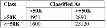
The confusion matrix which is used for generating the prediction performance is given below in Table 9.
Time taken to build model 0.03 seconds
Correctly classified instances 27380
(84.0883%)
Incorrectly classified instances 5181
(15.9117%)
Mean Absolute Error 0.1706
TABLE9
CONFUSIONMATRIXFORDECISIONTREE(J48)CLASSIFIER
Class Classified As
>50K <=50K
>50K 4951 2890
<=50K 1600 23120
The ROC curve is also shown below. The area under the ROC curve is 0.891.
Feature selection is also performed to find out if there exist a subset which leads to better performance of the classifier. But instead of exhaustive search, best-first search is used in this case as the runtime of the former was not acceptable.
The WEKA run selected the following 12 features out of 14 which form the subset for obtaining maximal
performance: age, workclass, fnlwgt, education,
education-num, marital-status, occupation, race, sex, capital-gain, capital-loss and hours-per-week. Hence feature selection process has excluded the two features, namely, relationship and native-country. The new performance results of the classifier is shown in Table 10.
TABLE 10
PREDICTION METRICS FOR DECISION TREE (J48) CLASSIFIER WITH FEATURE SELECTION
Class
Performance Metrics
TP Rate
FP Rate
Preci sion
Recal l
F-Meas
ure
ROC Area
>50K 0.638 0.067 0.752 0.638 0.69 0.89
<=50K 0.933 0.362 0.89 0.933 0.911 0.89
Wt.
Avg. 0.862 0.291 0.857 0.862 0.858 0.89
It is evident from the table that feature selection process has improved the prediction accuracy figures for class >50K. The overall ROC Area remains same though. Some other relevant performance measures are shown in Table 11 below.
TABLE 11
OTHER METRICS FOR DECISION TREE (J48) CLASSIFIER WITH FEATURE SELECTION
Time taken to build model 1.79 seconds
Correctly classified
instances
28075 (86.2228%)
Incorrectly classified
instances
4486
(13.7772%)
Mean Absolute Error 0.1934
Root Mean Squared Error 0.3201
Size of the tree 874
It is observed that due to introduction of feature selection there is a marginal improvement in time taken to build model as well as percentage of correctly classified instances. The size of the tree has also increased.
The confusion matrix which is used for generating the prediction performance is given below in Table 12.
TABLE12
CONFUSIONMATRIXFORDECISIONTREE(J48)CLASSIFIER
WITHFEATURESELECTION
Class Classified As
>50K <=50K
>50K 5001 2840
<=50K 1646 23074
C. Results for Support Vector Machine (SVM) Classification Algorithm
For SVM engine, the UCI dataset is also run with 10-fold cross-validation. But the model build time is much worse than naïve-Bayes and Decision Tree algorithms. Also the prediction performance numbers are worse than naïve-Bayes and Decision tree. Various metrics of its prediction accuracy and performance as reported by WEKA is provided below in Table 13.
TABLE13
PREDICTIONPERFORMANCEMETRICSFORSVMCLASSIFIER
Class
Performance Metrics
TP Rate
FP Rate
Preci sion
Recal l
F-Meas
ure
ROC Area
>50K 0.569 0.062 0.744 0.569 0.645 0.753
<=50K 0.938 0.431 0.873 0.938 0.904 0.753
Wt.
Avg. 0.849 0.342 0.842 0.849 0.842 0.753
It can be observed from Table 13 that ROC Area is much worse compared to naïve-Bayes and decision tree classifier. Some other relevant metrics are also shown in Table 14.
TABLE 14
OTHER METRICS FOR SVM CLASSIFIER
Time taken to build model 521.77 seconds
Correctly classified instances 27645
(84.9022%)
Incorrectly classified instances 4916
(15.0978%)
Mean Absolute Error 0.151
Root Mean Squared Error 0.3886
It can be seen that model build time is exponentially higher compared to naïve-Bayes and decision tree classifiers.
The confusion matrix which is used for generating the prediction performance is given below in Table 15.
TABLE15
CONFUSIONMATRIXFORSVMCLASSIFIER
Class Classified As
>50K <=50K
>50K 4458 3383
<=50K 1533 23187
The ROC curve is shown below. The area under ROC curve is 0.753 which is much less than naïve-Bayes and decision tree classifier.
As the performance figures of SVM engine is not acceptable, further experimentation using feature selection is not conducted.
D. Results for Bayesian Belief Network Classification Algorithm
For Bayesian network engine, the UCI dataset is also run with 10-fold cross-validation. The performance numbers are reported below in Table 16.
TABLE 16
PREDICTION PERFORMANCE METRICS FOR BAYESIAN NETWORK CLASSIFIER
Class
Performance Metrics
TP Rate
FP Rate
Preci sion
Recal l
F-Meas
ure
ROC Area
>50K 0.797 0.149 0.63 0.797 0.704 0.916
<=50K 0.851 0.203 0.93 0.851 0.889 0.916
Wt.
Avg. 0.838 0.19 0.857 0.838 0.844 0.916
It is evident that Bayesian network classifier performance in terms of ROC Area is much better compared to naïve-Bayes, decision tree and SVM based classifiers. Additionally, the gap in the prediction accuracy figures for both classes have reduced and performance of class >50K seems to have improved with Bayesian network. Some other relevant figures are also given in Table 17.
TABLE 17
OTHER METRICS FOR BAYESIAN NETWORK CLASSIFIER
Time taken to build model 0.34 seconds
Correctly classified instances 27295
(83.8273%)
Incorrectly classified
instances
5266 (16.1727%)
Mean Absolute Error 0.1766
Root Mean Squared Error 0.3427
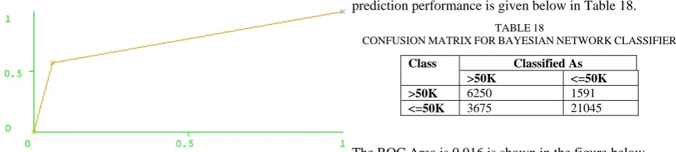
The confusion matrix which is used for generating the prediction performance is given below in Table 18.
TABLE18
CONFUSIONMATRIXFORBAYESIANNETWORKCLASSIFIER
Class Classified As
>50K <=50K
>50K 6250 1591
<=50K 3675 21045
As the results with Bayesian network look promising, further experimentation with feature selection is also performed using the Best-First scheme and ClassifiedSubsetEval of WEKA.
The WEKA run selected the following 6 features out of 14 which form the subset for obtaining maximal performance: age, education, occupation, occupation, relationship, capital-gain and capital-loss. The new performance results of the classifier is shown in Table 19 below.
TABLE 19
PREDICTION PERFORMANCE METRICS FOR BAYESIAN NETWORK CLASSIFIER WITH FEATURE SELECTION
Class
Performance Metrics
TP Rate
FP Rate
Preci sion
Recal l
F-Meas
ure
ROC Area
>50K 0.682 0.082 0.725 0.682 0.703 0.915
<=50K 0.918 0.318 0.901 0.918 0.909 0.915
Wt.
Avg. 0.861 0.261 0.859 0.861 0.86 0.915
It is evident from the table that feature selection process has not improved the prediction accuracy figures much. The overall ROC Area remains same, a little less at 0.915. Some other relevant performance measures are shown in Table 20 below.
TABLE 20
OTHER METRICS FOR BAYESIAN NETWORK CLASSIFIER WITH FEATURE SELECTION
Time taken to build model 0.2 seconds
Correctly classified instances 28044
(86.1276%)
Incorrectly classified
instances
4517 (13.8724%)
Mean Absolute Error 0.1843
Root Mean Squared Error 0.3116
It is observed that due to introduction of feature selection
there is improvement in time taken to build model as well
as percentage of correctly classified instances.
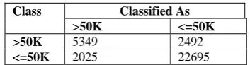
The confusion matrix which is used for generating the prediction performance is given below in Table 21.
TABLE 21
CONFUSION MATRIX FOR BAYESIAN NETWORK CLASSIFIER WITH FEATURE SELECTION
Class Classified As
>50K <=50K
>50K 5349 2492
<=50K 2025 22695
The ROC curve is shown below.
E. Results for Neural Network Classification Algorithm
The neural network classifier of WEKA (Multi-Layer Perceptron) is run on the UCI dataset with 10-fold cross-validation. The performance numbers are reported below in Table 22.
TABLE 22
PREDICTION PERFORMANCE METRICS FOR NEURAL NETWORK CLASSIFIER
Class
Performance Metrics
TP Rate
FP Rate
Preci sion
Recal l
F-Meas
ure
ROC Area
>50K 0.621 0.105 0.652 0.621 0.636 0.874
<=50K 0.895 0.379 0.882 0.895 0.888 0.874
Wt.
Avg. 0.829 0.313 0.826 0.829 0.827 0.874
It is observed that the prediction accuracy performance of neural network engine is worse than all other engines except SVM classifier. In addition, the model build time is even 3X worse than the performance of SVM classifier as shown in Table 23 below.
TABLE 23
OTHER METRICS FOR NEURAL NETWORK CLASSIFIER
Time taken to build model 1578.11
seconds
Correctly classified instances 26991
(82.8936%)
Incorrectly classified
instances
5570 (17.1064%)
Mean Absolute Error 0.1806
Root Mean Squared Error 0.3712
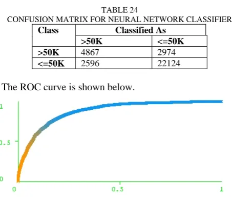
TABLE 24
CONFUSION MATRIX FOR NEURAL NETWORK CLASSIFIER
Class Classified As
>50K <=50K
>50K 4867 2974
<=50K 2596 22124
The ROC curve is shown below.
As the model build time is much more than the other classification engines, further experimentation with feature selection is not undertaken in this case.
V. SUMMARY OF COMPARATIVE ANALYSIS AND
CONCLUSION
The following table (Table 25) presents a consolidated summary of all the performance metrics of various
classifiers discussed in the previous section. Although it is evident that there is no clear winner in terms of all the parameters, yet, the decision tree classifier is possibly the best classifier in terms of most of the metrics. This table shows the numbers for the classifiers when they are run without any feature selection. Secondly, the prediction accuracy figures correspond to the weighted average of figures obtained for two classes, namely, >50K and <=50K.
The numbers shown in Table 25 clearly shows that Bayesian network and decision tree classifiers perform much better in predicting the salary class (>50K, <=50K) in UCI census dataset. The following chart shows the graphical representation of some important parameters given in Table 25. The reason for decision tree classification algorithm’s better performance lies in the basic structure of the features used in this dataset. Secondly, Bayesian network is generally found to perform reasonably well for various classes of classification problems and hence it is no surprise that it has performed well in this case also.
With feature selection taken into account (Table 26), the figures of Decision tree and Bayesian network classifiers are found to be better than the remaining ones.
TABLE 25
COMPARISON OF PERFORMANCE METRICS FOR VARIOUS CLASSIFIERS
Metrics
Classifier
Naïve-Bayes Decision Tree Bayesian Network SVM Neural network
TP Rate 0.834 0.862 0.838 0.849 0.829
FP Rate 0.382 0.295 0.19 0.342 0.313
Precision 0.825 0.857 0.857 0.842 0.826
Recall 0.834 0.862 0.838 0.849 0.829
F-Measure 0.824 0.858 0.844 0.842 0.827
ROC Area 0.892 0.891 0.916 0.753 0.874
Correctly classified instances 27165 (83.428%) 28071 (86.2105%) 27295 (83.8273%) 27645 (84.9022%) 26991 (82.8936%)
Time taken to build model 0.15 sec 1.85 sec 0.34 sec 521.77 sec 1578.11 sec
RMSE 0.3723 0.3196 0.3427 0.3886 0.3712
TABLE 26
COMPARISON OF PERFORMANCE METRICS WITH FEATURE SELECTION
Metrics Classifier
Naïve-Bayes Decision Tree Bayesian Network
TP Rate 0.841 0.862 0.861
FP Rate 0.379 0.291 0.261
Precision 0.832 0.857 0.859
Recall 0.841 0.862 0.861
F-Measure 0.83 0.858 0.86
ROC Area 0.896 0.891 0.915
Correctly classified instances 27380 (84.0883%) 28075 (86.2228%) 28044 (86.1276%)
Time taken to build model 0.03 sec 1.79 sec 0.2 sec
RMSE 0.3567 0.3201 0.3116
The comparison is shown graphically in the following diagram as well.
The comparative measures reported in Table 25 and 26 are also statistically validated at 5% significance level using WEKA Experimenter and for most of them Bayesian Network and Decision Tree classifier metrics have been found to be superior to those reported by other classifiers. The above findings show that decision tree and Bayesian belief network offer comparatively better performance for prediction of salary classes. For real life data, preference could be given to these machine learning algorithms while deciding the salary classes. The difference of real life salary data with UCI census dataset will be that the former will be more specific to a company and each tuple will invariably contain performance levels and some more company specific parameters. Although it is difficult to predict with 100% accuracy that decision tree and Bayesian network will perform better even on real company specific data of employees just based on this experiment, at least a basic pattern can be conjectured.
VI.FUTURE WORK
The future work would involve gathering real life company data and run salary prediction using the algorithms described above and verify the findings of this experiment. One possible analysis which could also be undertaken is to augment UCI census dataset by including performance attribute (using random generation or some other heuristics) and then run the machine learning algorithms in WEKA. This would have made the current experiment almost equivalent to real life salary prediction and the findings more relevant to employee salary prediction problem.
Additionally, one of the issues regarding over-fitting avoidance of algorithmic models, remain to be tested for this experiment. As we have noted earlier, the UCI census dataset is unbalanced with 70% belonging to <=50K category which could lead to bias in prediction. This could have been addressed using SMOTE filter of WEKA or by random under-sampling. It should be noted that the ensemble methods such as Bagging, AdaBoost, Voting (with majority votes) etc. has also been run as part of this experiment without any further improvement of classification performance which are reported in previous sections for individual classifiers..
Although in this paper the salary prediction problem is modelled as a classification problem, in real life, sometimes the managers may require exact value of the predicted salary. In that case, the same problem may be modelled as regression problem with salary being the dependent variable and the rest as independent variables. This kind of regression modelling can be taken up in future as well. Overall, this work can be utilized and extended to make enterprise compensation management more efficient by introducing automation of the salary prediction process.
ACKNOWLEDGMENT
First of all, I am thankful to the faculties of IIM Indore who inspired me to publish this work which is essentially the outcome of a term paper. Secondly, I would take this opportunity to acknowledge the sustained support extended to me by my wife, daughter and parents to complete this work.
BIBLIOGRAPHY
[1] University of California, I. (1994). UCI census dataset. Retrieved from UCI Machine Learning
Repository:
https://archive.ics.uci.edu/ml/datasets/Census+Inc ome
[2] Waikato, U. o. (n.d.). WEKA. Retrieved from http://www.cs.waikato.ac.nz/ml/weka/