Simulations of SH wave scattering due to cracks by the 2-D finite difference
method
Yuji Suzuki1∗, Jun Kawahara2, Taro Okamoto3, and Kaoru Miyashita2
1Graduate School of Science and Engineering, Ibaraki University, Mito 310-8512, Japan 2Faculty of Science, Ibaraki University, Mito 310-8512, Japan
3Department of Earth and Planetary Sciences, Tokyo Institute of Technology, Tokyo 152-8551, Japan (Received April 5, 2005; Revised October 11, 2005; Accepted October 31, 2005; Online published May 12, 2006)
We simulate SH wave scattering by 2-D parallel cracks using the finite difference method (FDM), instead of the popularly used boundary integral equation method (BIEM). Here special emphasis is put on simplicity; we apply a standard FDM (fourth-order velocity-stress scheme with a staggered grid) to media including traction-free cracks, which are expressed by arrays of grid points with zero traction. Two types of accuracy tests based on comparison with a reliable BIEM, suggest that the present method gives practically sufficient accuracy, except for the wavefields in the vicinity of cracks, which can be well handled if the second-order FDM is used instead. As an application of this method, we also simulate wave propagation in media with randomly distributed cracks of the same length. We experimentally determine the attenuation and velocity dispersion induced by scattering from the synthetic seismograms, using a waveform averaging technique. It is shown that the results are well explained by a theory based on the Foldy approximation for crack densities of up to about 0.1. The presence of a free surface does not affect the validity of the theory. A preliminary experiment also suggests that the validity will not change even for multi-scale cracks.
Key words:Scattering, cracked media, finite difference methods, attenuation, dispersion.
1.
Introduction
It is well known that the Earth’s interior, especially the lithosphere, has considerably strong short-wavelength het-erogeneities that scatter the seismic waves and thereby cause phenomena such as the scattering attenuation, the de-lay of the arrival times, and the generation of coda waves (e.g., Sato and Fehler, 1998). For revealing the short-wavelength heterogeneous structures in the Earth, it is im-portant to understand theoretically how they act on wave-fields.
For this purpose, two types of heterogeneity models are preferably considered; random spatial fluctuations of medium parameters (called random media), and spatial dis-tributions of discrete scatterers such as cracks, inclusions, or cavities. The wave propagation and scattering in media with such heterogeneities have been studied both analyti-cally and numerianalyti-cally. When calculating wavefields in ran-dom media, one usually uses ran-domain-type methods, among which the finite difference method (FDM) may be the most popular because of its tractability (e.g., Frankel, 1989; Gib-son and Levander, 1990; Jannaudet al., 1991a, b; Ikelleet al., 1993; Roth and Korn, 1993; Samuelides and Mukerji, 1998; M¨uller and Shapiro, 2001; Saitoet al., 2003). In con-trast, when dealing with discrete scatterers, boundary-type
∗Now at: Systemlab Corporation, Tokyo 167-0043, Japan.
Copyright cThe Society of Geomagnetism and Earth, Planetary and Space Sci-ences (SGEPSS); The Seismological Society of Japan; The Volcanological Society of Japan; The Geodetic Society of Japan; The Japanese Society for Planetary Sci-ences; TERRAPUB.
methods such as the boundary integral equation method (BIEM) has been preferred (e.g., Bouchon, 1987; Coutant, 1989; Beniteset al., 1992, 1997; Muraiet al., 1995; Pointer et al., 1998; Kelner et al., 1999; Liu and Zhang, 2001; Yomogida and Benites, 2002); the application of the FDM is rather restricted (see below as to the references). It may be because the BIEM is generally considered to have advan-tages over the FDM in the computational accuracy when dealing with discrete heterogeneities (e.g., Benites et al., 1992; Liu and Zhang, 2001), and in the great flexibility on the shapes of scatterers. However, the BIEM has also some shortcomings. For example, it cannot easily to be applied to media with discrete scatterers when the surrounding ma-trices have velocity or density heterogeneities. Moreover, its computational costs rapidly increase with the increas-ing number of scatterers; its computer program could be also rather hard for beginners to code. Since the FDM is suitable in these points, it is meaningful to apply it to the scattering by discrete scatterers if it gives practically suffi-cient accuracy with reasonable computational costs. One of the purposes of our study is to clarify this point concerning cracks.
The key to the FDM simulations of scattering by cracks (or fractures) is how we incorporate the cracks into the computational grids. Coates and Schoenberg (1995) pro-posed a technique in which materials in the grid cells inter-sected by fractures are modeled by equivalent homogeneous anisotropic materials, on the basis of the theory of Muiret al.(1992); here the fractures are modeled by thin weak elas-tic layers embedded in a surrounding matrix. The merit of
this technique is that the surfaces of fractures can take ar-bitrary angles to the grids. It was adopted by Vlastoset al. (2003) in their simulations of P-SV wave scattering in 2-D cracked media. Van Barenet al.(2001) and van Antwerpen et al.(2002) developed another technique in which cracks are replaced by distributed point sources of scattered waves. This is a hybrid method with the BIEM, that is used for eval-uating the source. Note that its application is restricted to relatively sparse microcracks, because it neglects multiple scattering and is also based on the long-wavelength approx-imation. Saenger et al. (2000) have expressed cracks by an assembly of the grid points with zero elastic constants and small densities. This is much simpler than the above techniques of crack incorporation and has an advantage in the flexibility on the crack shapes. It requires, however, a rotated staggered grid they proposed to make the computa-tions stable. Using it, Saenger and Shapiro (2002) treated wave propagation in 2-D media with intersecting cracks. Saengeret al.(2004) further extended this approach to 3-D cases. Note that Hong and Kennett (2002) also incorporated a fluid-filled crack in the grid in a similar manner, to which their wavelet-based method was applied.
In comparison with the above-mentioned techniques, special emphasis is put on the simplicity of the simulation technique we adopt. Here we treat 2-D SH (or acoustic) wave scattering due to traction-free cracks. For this pur-pose, we adopt a standard velocity-stress FDM (Virieux, 1984; Levander, 1988). We express cracks just by arrays of grid points with zero traction. Note that this is a natural extension of the simulations of crack propagation based on the velocity-stress FDM originated by Madariaga (1976), in which the boundary conditions on the crack planes can be directly given. Indeed, Fehler and Aki (1978) successfully applied Madariaga’s scheme to the diffraction by a single crack in a full space, where they divided the problem into a pair of mixed boundary value problems in half spaces and then solved them. Such a manner, however, has little ap-plicability to many non-coplanar cracks that can be easily treated by the present method. For validating it, we perform two types of accuracy tests based on the comparison with BIEM calculations (Murai et al., 1995). First, we calcu-late the displacement discontinuity along an isocalcu-lated crack caused by incident harmonic waves. Second, we synthe-size seismograms of waves scattered by clusters of several cracks at distant stations. We then discuss the numerical errors of the FDM calculations, assuming the BIEM coun-terparts to be exact. We will show that the present method gives practically sufficient accuracy. Note that dealing with 2-D SH waves may not be very practical, but it is our scope to validate the present method sufficiently in such a simple case; the extension to P-SV waves in 2-D cracked media will be given in a later paper.
An interesting topic on cracked media may be the attenu-ation and velocity dispersion of waves propagating therein. Theoretically, they can be predicted by a stochastic theory based on Foldy’s (1945) approximation (Kikuchi, 1981a, b; Yamashita, 1990; Kawahara and Yamashita, 1992; Kawa-hara, 1992; Zhang and Gross, 1997). This approximation is based on the assumption that many scatterers are distributed randomly and sparsely (Ishimaru, 1978), and it is expected
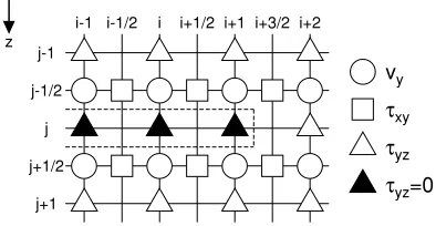
vy
τxy
τyz
τyz=0 j-1
j-1/2
j
j+1/2
j+1
i-1 i-1/2 i i+1/2 i+1 i+3/2 i+2 x
z
Fig. 1. Staggered grid and implementation of cracks. Antiplane (y-component) velocity and density are defined at the points with cir-cles. Antiplane shear stresses,τx yandτyzare defined at the points with
squares and triangles, respectively, at both of which rigidity is also de-fined. The region enclosed by the dotted line corresponds to a crack where the solid triangle denote the points withτyz=0.
to give results that are accurate to the first order in the dis-tribution density (Keller, 1964). However, its actual validity limit with respect to the density is not very clear. Using their BIEM, Murai et al.(1995) simulated SH wave scattering by 2-D cracks and experimentally determined the scatter-ing attenuation and dispersion, thus validatscatter-ing the Foldy ap-proximation theory as long as the crack density is relatively low (<0.02). Unfortunately, the ordinary peak picking tech-nique as they used in measurement will not work for dense crack distributions, because the initial motions of propa-gating waves will be often distorted too much to pick the peaks properly. As an application of the present simulation method, we perform here numerical experiments as Murai et al.(1995) did, though we adopt an alternative waveform averaging method. We simulate SH wave propagation in media with randomly distributed cracks, and determine the attenuation and dispersion from the spectral changes of av-eraged seismograms. We show that these parameters are obtained stably, even for rather dense crack distributions, thereby investigating the validity limit of the theory. This is another purpose of this paper and we will show that the theory remains valid, even for considerably high crack den-sities.
This paper is organized as follows. In the next section, we outline the FDM that we adopt, including the imple-mentation of cracks. We validate the method in Section 3 through the two accuracy tests. On the basis of the numer-ical experiments using it, we then investigate the validity of the Foldy approximation theory in Sections 4 and 5; the former section is focused on the validity limit of the the-ory, assuming identical cracks, whereas the latter concerns cracks with variable lengths. A discussion and conclusions are presented in the last section.
2.
Finite Difference Method
stag-gered grid (Fig. 1). Here the x-, y- andz-axes are taken in the horizontal, antiplane, and vertical directions, respec-tively. Note that the grid spacings in thex- andz-directions are assumed to have the same lengthh.
We assume that any crack is horizontal (parallel to thex -axis) and traction-free and is incorporated into the grid just by imposing the shear stress τyz = 0 on the horizontally
arrayed grid points (Fig. 1). As mentioned in Section 1, this may be analogous to the method of Fehler and Aki (1978) in that a Neumann problem is explicitly set; although they transformed the problem into a pair of mixed problems, we solve it in a straightforward way. We define the crack tips as the leftmost and rightmost points of the array (e.g., the grid point(i +1,j)in Fig. 1); though it may be also possible to define them as the positions half a grid spacing outside these grid points (e.g.,(i+3/2,j)), it is confirmed that the difference is negligible for sufficiently small grid spacings as expected.
In any simulation performed, a plane wavelet is assumed to propagate upward (in the negative z-direction) from be-low and be normally incident on cracks. Then velocity seis-mograms are synthesized at specified grid points, which are finally integrated with the trapezoidal rule to yield the dis-placement seismograms. Concerning the artificial bound-aries of the whole grid (model space), we again impose sim-ple conditions. The cyclic boundary condition is applied to the left and right ends to approximately express an infinitely long cracked layer. A standard absorbing boundary condi-tion of Clayton and Engquist (1977) is assumed along the bottom end. The condition of the top end is chosen between the absorbing or traction-free boundary conditions, depend-ing on simulations. Although artificial reflections from the absorbing boundaries cannot be perfectly erased, we actu-ally analyze the portions of seismograms not contaminated with them.
Hereafter, the shear wave velocity and the density of the background material, β and ρ, are set to be unity. We also assume that all the cracks have the same half length a = 1, except in Section 5 where we consider a distribu-tion of crack lengths. The values of other parameters are normalized with them. The grid spacinghare chosen to satisfy the ordinary sampling criterion
h < β/n ful, (1)
where n is 5 and 10 for the fourth- and second-order schemes, respectively, and ful is the effective upper limit
of the frequency band of waves.
3.
Accuracy Tests
3.1 Crack displacement discontinuity
In this section, we compare the results of our FDM sim-ulations with those given with the frequency-domain BIEM of Murai et al.(1995), thus trying to validate the present method. In order to treat the results of the BIEM as the cor-rect answers, we pay special attention to their accuracy; i.e., we discretize the crack planes finely so that the discretiza-tion intervalsin the BIEM may be much smaller than not only the crack length and the wavelength but also the dis-tances between neighboring cracks (namely, the minimum distance between two crack planes). Actually, we choose
s=0.0025a. In the first test, we check the validity of the present method through calculation of displacement discon-tinuity along a single crack, caused by the normal incidence of harmonic SH waves. This was analytically solved by Mal (1970), whose results have often been used by several au-thors to validate their own BIEM. Yamashita (1990), among others, developed a BIEM algorithm for treating an isolated crack, which reproduces Mal’s results quite accurately. It was extended by Muraiet al.(1995) to treat many cracks. Its code is used here.
Now let us calculate the results corresponding to Mal’s (1970) using the present FDM. Consider an isolated crack with the length 2a, upon which a quasi-monochromatic wave train
u0(x,z,t)=H(kz+ωt)sin(kz+ωt) (2)
normally impinges; here ω = 2πf, f is the frequency, k = ω/β is the wavenumber, and H( )is the step func-tion. This causes the oscillation of the crack faces, and ap-proaches the stationary state with the lapse time. We eval-uate the amplitudes of the oscillatory displacement discon-tinuity along the crack when the oscillation appears almost stationary. Since the displacement discontinuity cannot be defined on the crack plane, we measure instead the differ-ences of the displacement seismograms calculated at the pairs of grid points just above and below the crack plane (e.g., the grid points(i,j ±1/2)in Fig. 1), and then take their amplitudes. The approximation errors due to the off-sets of the measurement points from the crack plane would be small ifhis sufficiently small.
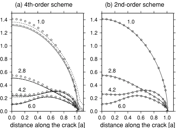
The results are summarized in Fig. 2(a), where the cases of the normalized wavenumberka=1.0, 2.8, 4.2, and 6.0 are examined after Mal (1970); the corresponding wave-lengths are 6.3a, 2.2a, 1.5a, and 1.0a, respectively. Here we set t = 0.003 (in unit of a/β) and impose the ab-sorbing boundary condition on the top end of the grid. On the basis of the fourth-order finite difference scheme, we repeatedly calculate the crack displacement discontinuity withh/a = 0.05, 0.025, and 0.0125. Note that the cor-responding results using the BIEM agree well with Mal’s. One might expect that the FDM results may approach the BIEM results (i.e., the exact solutions) ash/adecreases; instead, they appear to converge on somewhat (several per-cents) smaller values on the whole. This may not be sur-prising if the nonlocality of the fourth-order finite differ-ence operator is considered, that is, the calculation of the particle velocity at a grid point (e.g.,(i,j+1/2)in Fig. 1) requires the stresses at the preceding time at, not only the neighboring points ((i,j),(i,j+1)and(i±1/2,j+1/2)), but also the points beyond them ((i,j−1),(i,j +2)and
0.0 0.2 0.4 0.6 0.8 1.0 1.2 1.4
0.0 0.2 0.4 0.6 0.8 1.0
distance along the crack [a] (a) 4th-order scheme
1.0
2.8
4.2
6.0
0.0 0.2 0.4 0.6 0.8 1.0 1.2 1.4
0.0 0.2 0.4 0.6 0.8 1.0
distance along the crack [a] (b) 2nd-order scheme
1.0
2.8
4.2
6.0
Fig. 2. Displacement discontinuity along a single crack due to normal incidence of harmonic SH waves, normalized with respect to the value at the center of the crack atka→0. The abscissas represent the distance from the center (in unit ofa). The curve parameters denoteka. The open circles indicate the calculations by the BIEM of Muraiet al.(1995), whereas the lines do the FDM calculations. (a) The solid, dashed, and dotted lines denote the calculations by the fourth-order scheme withh/a=0.0125, 0.025, and 0.05, respectively. (b) The solid lines denote the calculations by the second-order scheme withh/a=0.01.
scheme. Now we assume that t = 0.00125 (a/β) and
h =0.01a. The results are indeed shown to agree with the BIEM calculations almost perfectly (Fig. 2(b)), support-ing the above discussion.
In summary, it is shown that crack displacement discon-tinuity, or wavefields in the vicinity of cracks, can be quite accurately evaluated using the second-order FDM. On the other hand, the fourth-order FDM systematically underesti-mates them, even for considerably small grid spacing, be-cause of the nonlocality of the finite difference operator. The relative errors, however, are several percents at most. If they are tolerable, the fourth-order FDM may be useful because of the lower computational costs due to its numeri-cal dispersion behavior better than that of the second-order one.
3.2 Scattered waveforms due to clustered cracks In the second test, we synthesize the displacement seis-mograms of scattered waves by clustered several cracks and examine the numerical errors. Here we adopt the fourth-order FDM only. We locate the cracks rather closely (with the intervals not very larger thanh) to see the effect on the accuracy of multiple scattering that would be strongly excited under such situations. In contrast, the observation points (hereafter, called stations) are located not very close to the cracks (with the distance larger than 2a), since the inaccuracy of “near-field” displacement calculated by the fourth-order FDM has been demonstrated in the above sub-section.
In the following, we sett = 0.005 (a/β) andh = 0.025a throughout; the absorbing boundary condition is again imposed on the top end of a grid (model space). Small numbers of cracks are closely located at around the center of the grid, and a plane wavelet is assumed to impinge on the cracks from below. Here we adopt a Ricker wavelet (second derivative of a Gaussian function; see Muraiet al., 1995 for
details), with the dominant frequency fc = 0.6 (in unit of
β/a) corresponding toka =3.77; here the corresponding wavelength λc = 1.67a is close to the crack length so
that scattering would occur strongly. We then synthesize the seismograms at horizontally arrayed stations above the cracks.
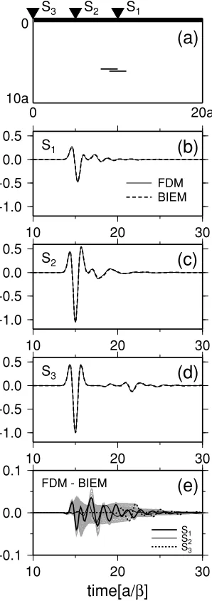
First, we treat a single crack for reference as shown in Fig. 3(a). Note that the center of the crack is located at
(x,z) = (10a,6.25a), defining the origin as the top left corner of the area. We evenly space 101 stations between
(x,z) = (0,0)and(0,20a), among which the stations at
(x,z)=(0,0),(5a,0)and(10a,0)are termed S3,S2and
S1, respectively. The FDM as well as BIEM seismograms
obtained at these three stations are depicted by Figs. 3(b) to 3(d). It is demonstrated that the single-scattered waves with relatively short durations follow the incident wavelets. They are separately recognized at the horizontally distant stationS3, whereas they overlap atS1right above the crack,
resulting in the deformation of the Ricker wavelet. In each case, the agreement between both seismograms is quite sat-isfactory, in spite of the discrepancy observed at the vicinity of cracks (Fig. 2(a)). This suggests that the errors due to the nonlocal finite difference operator would not strongly af-fect the “far-field” displacement. In order to closely look into the difference between the FDM and BIEM traces, we define here a normalized residual trace as
R(t)=uFDM(t)−uBIEM(t)/maxuBIEM(t), (3)
where uFDM and uBIEM are the FDM and BIEM traces, respectively.
0
10a
0 20a
S3 S2 S1
(a)
-1.0 -0.5 0.0 0.5
10 20 30
(b)
FDM BIEM S1
-1.0 -0.5 0.0 0.5
10 20 30
(c)
S2-1.0 -0.5 0.0 0.5
10 20 30
(d)
S3-0.1 0.0 0.1
10 20 30
time[a/
β
]
(e)
FDM - BIEMS1
S2
S3
Fig. 3. Comparison of seismograms based on the FDM and BIEM simu-lations. (a) Geometry of the simulation model examined. Here a single crack is located, above which 101 stations are horizontally spaced (the thick horizontal line). Note thath =0.025a. (b) FDM and BIEM traces at the stationS1, indicated in (a), normalized with the maximum amplitude of the initial wavelet. (c) As for (b) except for the stationS2. (d) As for (b) except for the stationS3. (e) Residual traces (difference between the FDM and BIEM traces). The thick solid, thin solid and dot-ted lines denote the residuals atS1,S2andS3, respectively. Residuals at all the other stations are indicated by the cloud of the fine gray lines.
may remark that the relative errors of the FDM traces are about 2% at most and, hence, considerably small.
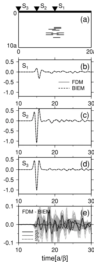
Next, we add one more crack at(x,z)=(9a,6a), where the interval between the cracks in the vertical direction is 0.25a = 10h = 0.15λc (Fig. 4(a)). This results in long
wave trains after the single-scattered waves, reflecting the reverberation between the cracks (Figs. 4(b) to 4(d)). Al-though the FDM and BIEM traces agree well, the ampli-tudes of the residual traces are rather larger than before (compare Fig. 4(e) with Fig. 3(e)). Careful observation of the traces in Figs. 4(b) to 4(d) suggests that these errors are mainly attributed to the slight phase offsets between the traces; except for these offsets, the errors in amplitude are
0
10a
0 20a
S3 S2 S1
(a)
-1.0 -0.5 0.0 0.5
10 20 30
(b)
FDM BIEM S1
-1.0 -0.5 0.0 0.5
10 20 30
(c)
S2-1.0 -0.5 0.0 0.5
10 20 30
(d)
S3-0.1 0.0 0.1
10 20 30
time[a/
β
]
(e)
FDM - BIEMS1
S2
S3
Fig. 4. Same as those in Fig. 3, except for two cracks closely located with the vertical interval 0.25a.
still quite small. To see the effect of the interval between the cracks on the FDM accuracy, we also reexamine the same model, except that the center of the upper crack is relocated at(x,z)=(9a,4.25a), with the vertical interval 2a =80h =1.2λc(Fig. 5(a)). Comparison of Figs. 4(b)
to 4(d) with Figs. 5(b) to 5(d) shows that the longer crack interval results in a somewhat longer duration of the rever-beration. Figures 4(e) and 5(e) suggest, however, that the FDM errors appear roughly unchanged, especially for the later waves. Concerning the direct waves, the errors are somewhat amplified at some stations (asS1).
0
10a
0 20a
S3 S2 S1
(a)
-1.0 -0.5 0.0 0.5
10 20 30
(b)
FDM BIEM S1
-1.0 -0.5 0.0 0.5
10 20 30
(c)
S2-1.0 -0.5 0.0 0.5
10 20 30
(d)
S3-0.1 0.0 0.1
10 20 30
time[a/
β
]
(e)
FDM - BIEMS1
S2
S3
Fig. 5. Same as those in Fig. 3, except for two cracks located with the vertical interval 2a.
that max|uBIEM(t)| in Eq. (3) (mostly, the amplitudes of the direct waves) largely varies with the stations (Figs. 6(b) to 6(d)). This would be responsible for the large spatial variation of the residuals shown in Fig. 6(e).
In summary, the fourth-order FDM generally gives con-siderably accurate seismograms (except for the vicinity of cracks), especially concerning the direct and early coda waves. The overall agreement between the FDM and BIEM (or correct) traces seems to be successful, though the rel-ative errors tend to somewhat increase with the increasing number of cracks (Figs. 3(e) to 6(e)). Moreover, the de-pendence of the errors on the intervals between cracks ap-pears much weaker. These characteristics would be prefer-able, especially when one deals with scattering by a large number of densely distributed cracks. Although we did not thoroughly pursue it here, the accuracy might be improved if the second-order FDM is totally adopted to the cracked media. In that case, however, we will probably need to use smaller grid spacings than those used in the present paper, because the second-order FDM is less accurate concerning
0
10a
0 20a
S3 S2 S1
(a)
-1.0 -0.5 0.0 0.5
10 20 30
(b)
FDM BIEM S1
-1.0 -0.5 0.0 0.5
10 20 30
(c)
S2-1.0 -0.5 0.0 0.5
10 20 30
(d)
S3-0.1 0.0 0.1
10 20 30
time[a/
β
]
(e)
FDM - BIEMS1
S2
S3
Fig. 6. Same as those in Fig. 3, except for 10 cracks closely clustered with the minimum vertical interval 0.25a.
the crack-free regions, due to its poorer numerical disper-sion relation.
We also point out that the FDM may be more cost-effective than the BIEM in treating many cracks, because the latter’s costs rapidly increase as the number of cracks increases, whereas the former’s costs are essentially un-changed (depending on the grid size instead). This is il-lustrated by a side experiment (not shown), whereswas taken to be five times larger than in the above experiments (i.e.,s =h/2 =0.0125a). It reduced the accuracy of the BIEM traces to the same level as for the FDM traces but remarkably saved the costs. Even then, the present BIEM needed larger CPU times than the FDM when more than 10 cracks were treated. This suggests the practicability of the present simulation method from the viewpoints of costs as well as of accuracy.
4.
Validation of the Foldy Approximation Theory
confirmed above. Using the method, we investigate here the validity of the Foldy approximation theory of Kawa-hara and Yamashita (1992) that predicts the scattering at-tenuation and velocity dispersion of elastic waves in 2-D media with identical parallel cracks. Here the prediction is stochastic in a sense that the theory is based on the mean wave formalism, i.e., it treats the ensemble average of real wavefields. Note that the theory also adopts an approxi-mation in which the waves effectively impinging on each scatterer (crack) are equal to the waves that would be ob-served without the scatterer. This approximation, first intro-duced by Foldy (1945), yields a closed equation for mean waves (called the Foldy–Twersky integral equation; Ishi-maru, 1978); Kawahara and Yamashita (1992) solved it to obtain the attenuation and phase velocity of the mean waves to the first order in the crack density. The approximation is sometimes considered as a kind of single scattering ap-proximation, since it does not take account of interactions between scatterers explicitly.
A similar trial to validate the theory of Kawahara and Yamashita (1992) was done by Murai et al.(1995) on the basis of a peak picking technique, in which the attenua-tion and phase velocity are determined from the amplitudes and travel times of the maximum peaks of bandpass-filtered seismograms and then averaged. Although the peak pick-ing technique is simple and practical in real seismic obser-vations, it also has some shortcomings. One of them is its less applicability to dense crack distributions, as mentioned in Section 1. In addition, its results depend on the choice of filter bandwidths. Another popular method may be to stack the amplitude spectra of individual seismograms, thereby estimating the averaged spectral change (e.g., Roth and Korn, 1993). The results, however, now depend on the time windows used for Fourier-transforming the seismograms, since no window perfectly separates the direct wave com-ponents from the seismograms. We also notice that none of these methods are conceptually consistent with the mean wave formalism. To overcome these problems, we adopt an alternative waveform-averaging method loyal to the formal-ism, as stated below.
First, we assume N cracks with the length 2a inside a rectangular area with the horizontal size W and vertical size L. Using a uniform random number series, the cracks are distributed inside the area almost randomly, except for the non-overlapping constraint that the interval between any two points belonging, respectively, to any two crack planes must be greater than 0.25a. Here the 2-D crack density is defined as = N a2/W L. Second, we array 100 stations
evenly along a horizontal line 2a above the top end of the crack distribution area. We then let a plane wavelet be vertically incident on the bottom end from below, and synthesize seismograms at the stations using the FDM. We adopt here an incident wavelet with the following source time function (first derivative of a Gaussian function; see Fig. 7):
u0(t)= −4πte−2πt2, (4)
whose amplitude spectrum is
F(ω)=√ω
Fig. 7. (a) Source time function of the incident wavelet used. The abscissa denotes time in unit ofa/β. (b) Amplitude spectrum of the wavelet as a function of normalized wavenumberka=ωa/β.
This is because the present wavelet has a broader spectral band than that of the Ricker wavelet, being more effective for the present purpose. We then repeat the above simu-lation for ND different realizations of the crack
distribu-tion that are stochastically identical but are generated using different random number series. Third, we average all the seismograms obtained for each realization. This means that spatial averaging is substituted for ensemble averaging, as-suming ergodicity. The results are then ensemble-averaged over theNDrealizations of the crack distribution; the final
result is termed “synthetic mean wave”. Fourth, the spec-trum of the mean wave is calculated. In doing this, we se-lect a time window that effectively includes the whole mean wave. If sufficiently many seismograms are stacked, the incoherent coda waves will be removed almost completely and, hence, the window width will not influence the results; actually, we choose ND enough to achieve this state. We
then evaluate the attenuation Q−1 and the phase velocity
v from the spectral ratio, C(f), of the mean wave to the initial wavelet that would be observed without the cracks. After some calculation, we obtain
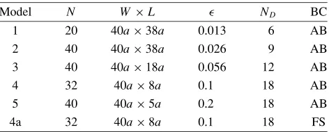
Table 1. Parameters of the crack distribution models used in simulations. BC indicates the boundary condition on the top end of the grid. AB indicates an absorbing boundary being settled above the station array. FS indicates a free surface being settled along the array.
Model N W×L ND BC
1 20 40a×38a 0.013 6 AB
2 40 40a×38a 0.026 9 AB
3 40 40a×18a 0.056 12 AB
4 32 40a×8a 0.1 18 AB
5 40 40a×5a 0.2 18 AB
4a 32 40a×8a 0.1 18 FS
wave and regard it as the estimation error. We also compute the waveform predicted by the Foldy approximation theory (“predicted mean wave”), using Eq. (6) with Q−1 andv given by the theory and then inverse Fourier-transforming. If the predicted mean wave coincides with the synthetic one within the error range, we regard their coincidence as sig-nificant.
In the following, we choose t = 0.005 (a/β) and
h = 0.025a throughout. Other parameters of the crack distribution models used are summarized in Table 1. An ex-ample of the realizations for each crack distribution model is depicted in Fig. 8.
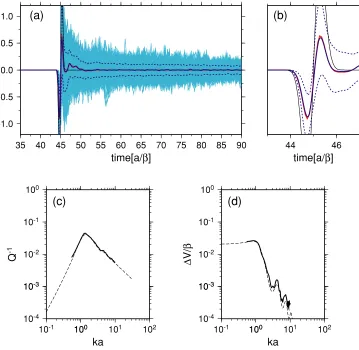
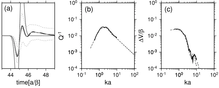
We first demonstrate the results for Model 1 (Fig. 9), that is, the case where the crack density ( = 0.013) is so low that the Foldy approximation is expected to be valid. In Fig. 9(a), we plot ND×100 seismograms used in the
analysis. Here we also show the trace of the synthetic mean wave and its standard deviation (error range) derived from the seismograms; the initial wavelet without the cracks is also plotted for reference (see also Fig. 9(b) as the close-up). Here one may clearly observe the attenuation on the direct wave part of the mean wave trace (44 < t < 46 in unit of a/β). The direct wave is also followed by a pulse of relatively long duration (around 46 < t < 50). However, the trace does not contain a coda-like long wave train, implying that the averaging process is successful in removing coda waves. We further plot the trace of the predicted mean wave in the figure. The coincidence of the synthetic and predicted mean waves is considerably good. This also suggests that the above-mentioned pulse, after the direct wave, should result from the waveform dispersion of the initial wavelet due to scattering. The values ofQ−1and
v/βderived from the both traces are plotted in Figs. 9(c) and 9(d) for 0.5 < ka < 10 (k = ω/β), respectively, where v = β −v is the phase velocity reduction due to scattering. The agreement between the experimental and theoretical values are fairly good on the whole, even including the ripple pattern ofv/βfor high wavenumbers, as may be expected from the above results. It may strongly support the validity of the Foldy approximation theory on cracked media, being consistent with the results of Muraiet al.(1995).
We next show the results for the models with denser dis-tributions (Models 2 to 5), focusing on the validity limit of the theory. Here, however, we skip the result for Model 2
-50 -40 -30 -20 -10
0 10 20 30 40 (a)
-50 -40 -30 -20 -10
0 10 20 30 40 (b)
-30 -20 -10
0 10 20 30 40 (c)
-20 -10
0 10 20 30 40 (d)
-15 -10
0 10 20 30 40 (e)
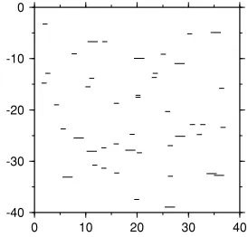
Fig. 8. Examples of crack distribution realizations for (a) Models 1 ( = 0.013), (b) 2 ( =0.026), (c) 3 ( = 0.055), (d) 4 ( = 0.1), and (e) 5 ( = 0.2). The axes denote length normalized witha. 100 stations are evenly spaced along the top end of each rectangular region, just below which is a gap with the thickness 2abetween the stations and the really cracked area.
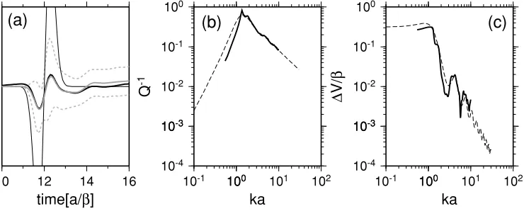
( =0.026), since it is almost the same as that for Model 1. The results for Models 3 and 4 with a relatively dense dis-tribution ( = 0.056 and 0.1) are shown in Figs. 10 and 11, respectively, where we may still recognize the fairly good agreement between the synthetic and theoretical re-sults in both the traces (Figs. 10(a), 11(a)) and Q−1 and
-1.0 -0.5 0.0 0.5 1.0
35 40 45 50 55 60 65 70 75 80 85 90
time[a/β]
(a)
44 46
time[a/β]
(b)
10-4 10-3 10-3 10-2 10-1 100
Q
-1
10-1 101000 101 102
ka
(c)
10-4 10-3 10-3 10-2 10-1 100
Δ
V/
β
10-1 101000 101 102
ka
(d)
Fig. 9. (a) Seismograms obtained for Model 1 ( =0.013). The cloud of thin light blue lines denotes all the synthetic seismograms. The solid blue curve indicates the synthetic mean wave, and the dotted blue curves do its standard deviation. The predicted mean wave is indicated by the red curve, though almost masked by the solid blue one. The thin black curve denotes the initial wavelet that would be observed without the cracks. (b) The close-up of the direct wave part in (a). The synthetic seismograms are omitted. (c)Q−1for the synthetic seismograms (thick solid curve). The prediction by the Foldy approximation theory is denoted by the dashed curve. (d) As for (d), except forv/β, wherevis the phase velocity reduction.
24 26 28
time[a/β]
(a)
10-4 10-3 10-3 10-2 10-1 100
Q
-1
10-1 101000 101 102 ka
(b)
10-4 10-3 10-3 10-2 10-1 100
Δ
V/
β
10-1 101000 101 102 ka
(c)
Fig. 10. Same as those in Fig. 9 except for Model 3 ( =0.056). The seismograms in the full range as Fig. 9(a) is omitted.
exp(−k Q−1x/2)as usual, where x is the travel distance.
Strictly, however, it is an approximation valid for weak at-tenuation, i.e., Q−1 1 (e.g., Aki and Richards, 2002). This will not be satisfied in the present case, where the max-imum value of Q−1 approximates to 1, probably making both the theory and measurement less reliable. This infer-ence appears to be supported by the distinct acausal motion of the predicted mean wave before the onset of the initial
wavelet without cracks (t ∼ 11), which deviates from the error range of the synthetic mean wave (Fig. 12(a)).
14 16 18 time[a/β]
(a)
10-4 10-3 10-3 10-2 10-1 100
Q
-1
10-1 101000 101 102 ka
(b)
10-4 10-3 10-3 10-2 10-1 100
Δ
V/
β
10-1 101000 101 102 ka
(c)
Fig. 11. Same as those in Fig. 10 except for Model 4 ( =0.1) as well as monochromatic drawing. In (a), the synthetic mean wave and its standard deviation are now indicated by gray lines, whereas the predicted mean wave is done by bold black line.
10 12 14 16
time[a/β]
(a)
10-4 10-3 10-3 10-2 10-1 100
Q
-1
10-1 101000 101 102 ka
(b)
10-4 10-3 10-3 10-2 10-1 100
Δ
V/
β
10-1 101000 101 102 ka
(c)
Fig. 12. Same as those in Fig. 11 except for Model 5 ( =0.2).
of the predicted mean wave (as well as the initial wavelet without cracks) is exactly duplicated on the surface. We also observe the experimental results similar to those for Model 4 (Fig. 11) on the whole. A noticeable difference is that the measured v/β are not stably determined for high wavenumbers. This may reflect the fact that the high-frequency coda waves are not sufficiently removed in this case, even though we assume hereND =18 as before (see
the ripples of the coda part of the synthetic mean wave for Model 4a, not seen for Model 4 (Fig. 13(d))). The ampli-tude of the direct waveform of the synthetic mean wave is also slightly different from that for Model 4, correspond-ing to the slightly larger values of the measuredQ−1in the dominant wavenumber range 0.2 < ka < 0.5. Such dis-crepancies should be regarded as the effects of a free sur-face, since any other conditions are unchanged, though they are rather small so that they are negligible.
In summary, one may say that the theory is valid for crack densities up to about 0.1 but probably not beyond it. The presence of a free surface does not change the conclusion. We remark that the real (though 3-D) crack densities of the crustal rock inferred from the shear-wave splitting analyses do not generally exceed 0.1, except for regions under some special conditions such as very near-surface layers or tec-tonically active regions (Crampin, 1994). We may therefore infer that the Foldy approximation theory may be applicable to most regions of the Earth’s crust, though more accurate
statements would require the researches on scattering in 3-D cracked media.
5.
Scattering Due to Cracks with Binary Lengths
com-14 16 18
time[a/
β
]
(a)
10-4 10-3 10-3 10-2 10-1 100
Q
-1
10-1 101000 101 102
ka
(b)
10-4 10-3 10-3 10-2 10-1 100
Δ
V/
β
10-1 101000 101 102
ka
(c)
16 20 24 28 32
time[a/
β
]
(d)
Fig. 13. Effect of a free surface. (a) to (c) are the same as for Figs. 10(a) to (c), except for Model 4a (Model 4 plus the free surface). (d) indicates the comparison among the coda traces for Models 4 (green curves), Models 4a (blue curves) and the corresponding predicted mean wave (red curve). The meanings of the solid and dotted curves are the same as for (a).
posed of identical cracks. This should be valid as long as the crack density is so low that one can neglect the higher-order terms in the crack density (e.g., Hudson, 1986).
We consider a random distribution of parallel cracks that are divided into two subgroups, each of which contains Nj
cracks with the length 2lja (j = 1,2), where a is now
a reference scale. Letting the distribution area beW ×L again, one may define the crack density in this case as
= 2
j=1
j, j =
Nj(lja)2
W L . (9)
Then the theoretical predictions of the attenuation and dis-persion may be given as
Q−1(ka)=
2
j=1
jQˆ(klja), v
β = 2
j=1 jv(ˆ
klja)
β ,
(10) where the caret means a prediction for identical cracks distributed with unit crack density. We assume here that N1 = 32, N2 = 12, andl1/l2 = 1/2; assigninga to the
mean crack length, then l1 = 11/14 andl2 = 11/7. We
choose the same values ofW,L,tandhas for Model 1; thereby the crack density is also the same ( =0.013). Con-cerning the boundary conditions and the values ofND,
how-ever, they are set as for Model 4a. We term this simulation model as Model 6; an example of the crack distribution re-alization is depicted in Fig. 14.
-40 -30 -20 -10 0
0 10 20 30 40
Fig. 14. Same as those in Fig. 8 except for Model 6 ( =0.013, with a free surface).
We show the results for Model 6 in Fig. 15. A notice-able feature is that the peak ofQ−1curve and the corner of
44 46 48 time[a/β]
(a)
10-4 10-3 10-3 10-2 10-1 100
Q
-1
10-1 101000 101 102 ka
(b)
10-4 10-3 10-3 10-2 10-1 100
Δ
V/
β
10-1 101000 101 102 ka
(c)
Fig. 15. Same as those in Fig. 11 except for Model 6. Note thatadenotes the mean crack length only in this case.
examples of validating the Foldy approximation theory for multi-scale scatterers.
6.
Discussion and Conclusions
In this paper, we applied a standard fourth-order velocity-stress FDM to the simulations of SH waves scattered by 2-D parallel cracks. We expressed traction-free cracks on the finite-difference grid in probably the simplest manner, i.e, assuming arrays of grid points with zero traction. We per-formed two types of accuracy tests of the method, on the basis of comparison with a reliable BIEM; one is the cal-culation of the displacement discontinuity along an isolated crack acted on by harmonic waves, and the other is syn-thesizing seismograms of waves scattered by several clus-tered cracks at somewhat distant stations. Both tests suggest that the fourth-order FDM yields practically sufficient accu-racy, except for the wavefields in the very vicinity of cracks, which can be well described by the second-order FDM.
The present method has some advantages over the BIEM. First of all, it has no limitation with respect to the variation of crack lengths, as we demonstrated above. Also men-tioned in Subsection 3.2, it could be more cost-effective when dealing with many densely distributed cracks, though the quantitative conclusions depend on many factors such as required accuracy. The most remarkable merit of the FDM would be, however, the ability to incorporate the back-ground heterogeneity in a straightforward manner. This would be the point that the BIEM is weak, since it is es-sentially applicable only to structures with their Green func-tions known. Although we did not show any examples here, the FDM could be readily applied to many seismological problems, such as waves trapped by a fault zone made of weak materials with many fractures. We also remark that the extensions of the present method concerning 2-D SH wave scattering to other types of waves is almost straight-forward; the extension to P-SV waves in 2-D cracked me-dia will be demonstrated in our next paper, as mentioned in Section 1.
On the other hand, the present method can deal with rather limited types of cracks, as the price of its high sim-plicity. For instance, only the cracks parallel to the grid lines (x- orz-directions) can be exactly (in the discretized numerical sense) treated by the present method. Incorpora-tion of inclined cracks into the grid retaining the
computa-tional accuracy, remains to be investigated. One of the can-didates for inclined cracks is the use of stairsteps of FDM grids; the stairstep approximation has been successfully ap-plied to the fluid-solid boundary with tangential discontinu-ity (e.g., van Vossenet al., 2002; Okamoto and Takenaka, 2005).
The present method has also been validated only for cracks with the traction-free condition, namely, empty cracks. They are not, of course, realistic in the crust. Thus the extensions of the method with respect to these points is required. For handling more general crack boundary condi-tions, the approach of Fehler and Aki (1978) might be use-ful. For evaluating the diffraction by a single crack filled with compressible inviscid fluid, they defined the boundary condition as the constitutive relation with respect to the dis-placement discontinuity and the resistance by the internal fluid, which was successfully solved using the FDM. We remark that it is essentially the same as the manner of Kawa-hara and Yamashita (1992) to deal with a crack filled with incompressible viscous fluid, that was adopted in the BIEM simulations of Muraiet al.(1995). We therefore infer that general compressible viscous fluid could be also treated in the same manner.
Acknowledgments. We deeply appreciate Yoshio Murai for pro-viding his BIEM code that is essential to the accuracy tests we carried out. The comments of Eiichi Fukuyama, Haruo Sato, and an anonymous reviewer helped us to improve the manuscript. All the figures in this paper were generated using the GMT software of Wessel and Smith (1998). This study was partially supported by the Earthquake Research Institute Cooperative Research Program (2000-B-07, 2003-B-04).
References
Aki, K. and P. G. Richards,Quantitative Seismology, 2nd edition, 699 pp., University Science Books, Sausalito, California, 2002.
Benites, R., K. Aki, and K. Yomogida, Multiple scattering of SH waves in 2-D media with many cavities,Pure Appl. Geophys.,138, 353–390, 1992.
Benites, R., P. M. Roberts, K. Yomogida, and M. Fehler, Scattering of elastic waves in 2-D media I. Theory and test,Phys. Earth Planet. Inter., 104, 161–173, 1997.
Bouchon, M., Diffraction of elastic waves by cracks or cavities using the discrete wavenumber method,J. Acoust. Soc. Am.,81, 1671–1676, 1987.
Clayton, R. and B. Engquist, Absorbing boundary conditions for acoustic and elastic equations,Bull. Seism. Soc. Am.,67, 1529–1540, 1977. Coates, R. T. and M. Schoenberg, Finite-difference modeling of faults and
fractures,Geophysics,60, 1514–1526, 1995.
Coutant, O., Numerical study of the diffraction of elastic waves by fluid-filled cracks,J. Geophys. Res.,94, 17805–17818, 1989.
Crampin, S., The fracture criticality of crustal rocks,Geophys. J. Int.,118, 428–438, 1994.
Fehler, M. and K. Aki, Numerical study of diffraction of plane elastic waves by a finite crack with application to location of a magma lens,
Bull. Seism. Soc. Am.,68, 573–598, 1978.
Foldy, L. L., The multiple scattering of waves. I. General theory of isotropic scattering by randomly distributed scatterers,Phys. Rev.,67, 107–119, 1945.
Frankel, A., A review of numerical experiments on seismic wave scatter-ing,Pure Appl. Geophys.,131, 639–685, 1989.
Gibson, B. S. and A. R. Levander, Apparent layering in common-midpoint stacked images of two-dimensionally heterogeneous targets,
Geophysics,55, 1466–1477, 1990.
Hong, T.-K. and B. L. N. Kennett, On a wavelet-based method for the numerical simulation of wave propagation,J. Comp. Phys.,183, 577– 622, 2002.
Hudson, J. A., A higher order approximation to the wave propagation constants for a cracked solid,Geophys. J. Roy. Astr. Soc.,87, 265–274, 1986.
Ikelle, L. T., S. K. Yung, and F. Daube, 2-D random media with ellipsoidal autocorrelation functions,Geophysics,58, 1359–1372, 1993. Ishimaru, A.,Wave Propagation and Scattering in Random Media, Vols. 1
and 2, 609 pp., Academic Press, New York, 1978 (reissued in 1997 by IEEE Press and Oxford Univ. Press, New York).
Jannaud, L. R., P. M. Adler, and C. G. Jacquin, Spectral analysis and inversion of codas,J. Geophys. Res.,96, 18215–18231, 1991a. Jannaud, L. R., P. M. Adler, and C. G. Jacquin, Frequency dependence
of the Q factor in random media,J. Geophys. Res.,96, 18233–18243, 1991b.
Kawahara, J., Scattering of P, SV waves by a random distribution of aligned open cracks,J. Phys. Earth,40, 517–524, 1992.
Kawahara, J. and T. Yamashita, Scattering of elastic waves by a fracture zone containing randomly distributed cracks,Pure Appl. Geophys.,139, 121–144, 1992.
Keller, J. B., Stochastic equations and wave propagation in random media,
Proc. Symp. Appl. Math.,16, 145–170, 1964.
Kelner, S., M. Bouchon, and O. Coutant, Numerical simulation of the propagation of P waves in fractured media,Geophys. J. Int.,137, 197– 206, 1999.
Kikuchi, M., Dispersion and attenuation of elastic waves due to multi-ple scattering from inclusions,Phys. Earth Planet. Inter.,25, 159–162, 1981a.
Kikuchi, M., Dispersion and attenuation of elastic waves due to multiple scattering from cracks,Phys. Earth Planet. Inter.,27, 100–105, 1981b. Levander, A. R., Forth-order finite-difference P-SV seismograms,
Geo-physics,53, 1425–1436, 1988.
Liu, E. and Z. Zhang, Numerical study of elastic wave scattering by cracks or inclusions using the boundary integral equation method,J. Comp. Acoust.,9, 1039–1054, 2001.
Madariaga, R., Dynamics of an expanding circular fault,Bull. Seism. Soc. Am.,66, 639–666, 1976.
Main, I. G., S. Peacock, and P. G. Meredith, Scattering attenuation and the fractal geometry of fracture systems,Pure Appl. Geophys.,133, 283– 304, 1990.
Mal, A. K., Interaction of elastic waves with a Griffith crack,Int. J. Engng. Sci.,8, 763–776, 1970.
Muir, F., J. Dellinger, J. Etgen, and D. Nichols, Modeling elastic fields across irregular boundaries,Geophysics,57, 1189–1193, 1992. M¨uller, T. M. and S. A. Shapiro, Most probable seismic pulses in single
realizations in two- and three-dimensional random media,Geophys. J. Int.,144, 83–95, 2001.
Murai, Y., J. Kawahara, and T. Yamashita, Multiple scattering of SH waves in 2-D elastic media with distributed cracks,Geophys. J. Int.,122, 925– 937, 1995.
Okamoto, T. and H. Takenaka, Fluid-solid boundary implementation in the velocity-stress finite-difference method,Zisin(J. Seism. Soc. Japan),57, 355–364, 2005 (in Japanese with English abstract and figures) Pointer, T., E. Liu, and J. A. Hudson, Numerical modelling of seismic
waves scattered by hydrofractures: application of the indirect boundary element method,Geophys. J. Int.,135, 289–303, 1998.
Roth, M. and M. Korn, Single scattering theory versus numerical mod-elling in 2-D random media,Geophys. J. Int.,112, 124–140, 1993. Saenger, E. H. and S. A. Shapiro, Effective velocities in fractured media:
a numerical study using the rotated staggered finite-difference grid,
Geophys. Prospect.,50, 183–194, 2002.
Saenger, E. H., N. Gold, and S. A. Shapiro, Modeling the propagation of elastic waves using a modified finite-difference grid,Wave Motion,31, 77–79, 2000.
Saenger, E. H., O. S. Kr¨uger, and S. A. Shapiro, Modeling the propaga-tion of elastic waves using a modified finite-difference grid,Geophys. Prospect.,52, 183–195, 2004.
Saito, T., H. Sato, M. Fehler, and M. Ohtake, Simulating the envelope of scalar waves in 2D random media having power-law spectra of velocity fluctuation,Bull. Seism. Soc. Am.,93, 240–252, 2003.
Samuelides, Y. and T. Mukerji, Velocity shift in heterogeneous media with anisotropic spatial correlation,Geophys. J. Int.,134, 778–786, 1998. Sato, H. and M. C. Fehler,Seismic Wave Propagation and Scattering in
the Heterogeneous Earth, 308 pp., Springer-Verlag, New York, 1998. Suzuki, Y., Simulations of seismic waves scattered by 2-D cracks using the
finite difference method, MSc thesis, Ibaraki University, Mito, 2004 (in Japanese).
Van Antwerpen, V. A., W. A. Mulder, and G. C. Herman, Finite-difference modeling of two-dimensional elastic wave propagation in cracked me-dia,Geophys. J. Int.,149, 169–178, 2002.
Van Baren, G. B., W. A. Mulder, and G. C. Herman, Finite-difference modeling of scalar-wave propagation in cracked media,Geophysics,66, 267–276, 2001.
Van Vossen, R., J. O. A. Robertsson, and C. H. Chapman, Finite-difference modeling of wave propagation in a fluid-solid configuration, Geo-physics,67, 618–624, 2002.
Viriuex, J., SH-wave propagation in heterogeneous media: velocity-stress finite difference method,Geophysics,49, 1933–1957, 1984.
Vlastos, S., E. Liu, I. G. Main, and X.-Y. Li, Numerical simulation of wave propagation in media with discrete distributions of fractures: effects of fracture sizes and spatial distributions,Geophys. J. Int.,152, 649–668, 2003.
Wessel, P. and W. H. F. Smith, New, improved version of the Generic Mapping Tools Released,EOS, Trans., Am., Geophys. Un.,79, 579, 1998.
Yamashita, T., Attenuation and dispersion of SH waves due to scattering by randomly distributed cracks,Pure Appl. Geophys.,132, 545–568, 1990. Yomogida, K. and R. Benites, Scattering of seismic waves by cracks with the boundary integral method,Pure Appl. Geophys.,159, 1771–1789, 2002.
Zhang, Ch. and D. Gross,On Wave Propagation in Elastic Solids with Cracks, 248 pp., Computational Mechanics, Southampton, UK, 1997.