Differential ionosphere modelling for single-reference long-baseline GPS
kinematic positioning
H. Dekkiche, S. Kahlouche, and H. Abbas
Geodesy Division, Space Techniques Center, Algerian Space Agency, Algiers, Algeria
(Received March 3, 2009; Revised July 30, 2010; Accepted November 16, 2010; Online published February 3, 2011)
The ionospheric effect is considered to be one of the most important error sources limiting the quality of GPS kinematic positioning. Over longer distances, differential ionospheric residuals become larger and may affect the ambiguity resolution process. We present here a Kalman-filter-based GPS ionosphere model for long-baseline kinematic applications. This observational model includes the differential ionosphere as an additional unknown factor with position coordinates and ambiguities, while the temporal correlations of the state vector are specified in the dynamic model. The temporal behaviour of ionospheric residuals is determined by the analysis of their autocorrelation function. This newly developed method was applied on a set of data collected by a roving receiver located offshore of Oran (Algeria). The results show that for baselines of about 80 km, the root mean square is at the level of a few centimetres. For tests of baselines of about 51 km, the comparison between short- and long-baseline solutions revealed that mean differences of a few millimetres and 2 cm are obtained for the horizontal coordinates and vertical component, respectively, and the standard deviation (σ) of differences on the scale of a few centimetres.
Key words: GPS kinematic positioning, long baseline, Kalman filter, differential ionosphere, temporal-correlation.
1.
Introduction
The development of the GPS kinematic technique has en-abled real-time accurate positioning of a mobile platform to be performed. For such accurate GPS kinematic position-ing, however, it is necessary to determine the integer num-ber of carrier phase cycles, which is called “integer ambi-guities”. Over short baselines, the double-difference (DD) technique can be applied to cancel out most of the corre-lated errors. Another option—and a common practice— is simply to disregard their effects. However, in the case of long-baseline kinematic positioning, the ionospheric ef-fect become increasingly more decorrelated, and it may af-fect the ambiguity resolution process, or even make it im-possible to compute (Vollathet al., 2000; Wielgoszet al., 2005). Therefore, reducing the differential ionospheric ef-fect is one of the most important steps towards improving ambiguity resolution and to achieve accurate medium- and long-range kinematic positioning (Odijk, 2000; Vollathet al., 2000; Kashaniet al., 2005; Wielgoszet al., 2005). In recent years, many approaches have been developed to en-able high-accuracy GPS kinematic positioning over longer distances (W¨ubbenaet al., 1996; Han, 1997; Raquet, 1998; Wanninger, 1999; Lachapelle et al., 2000; Odijk et al., 2000; Hernandez-Pajareset al., 2000; Cannonet al., 2001; Rizos, 2002; Huet al., 2003; Chenet al., 2004; Wielgosz
et al., 2004, 2005). All of these investigations involve the
Copyright cThe Society of Geomagnetism and Earth, Planetary and Space Sci-ences (SGEPSS); The Seismological Society of Japan; The Volcanological Society of Japan; The Geodetic Society of Japan; The Japanese Society for Planetary Sci-ences; TERRAPUB.
doi:10.5047/eps.2010.11.004
use of multi-reference stations. However, a network of GPS reference stations is not always available and its im-plementation is costly. In addition, in certain cases (e.g., marine long-baseline applications), interpolated corrections are not reliable because the rover receiver is usually outside the network coverage area. A new approach based on a single-reference-station mode has been published by Kim and Langley (2007) that nullifies the effect of the differen-tial ionosphere in an ambiguity search process; this method provides a number of interesting results.
In this paper, GPS kinematic positioning is implemented in a single-reference-station mode. Our approach is based on the use of the Kalman filtering method to estimate the differential ionospheric delay as a state with unknown posi-tion coordinates and ambiguities. To model the ionospheric delays as a state, an additional parameter for each satellite must be included in the observation equations that involves a singularity of the equation system (i.e., the number of un-known parameters becomes greater than the number of ob-servations). To overcome this problem, the redundancy is increased by using dual-frequency carrier phases (L1 and
L2) and code pseudo-range (P1, P2and C/A) measurements.
The Kalman filtering method is based on the use of two models: the observation model (for updating or correction) and the underlying dynamic model (for prediction). The observation model describes the relationship between the observations and unknown parameters, while the dynamic model allows the user to predict the state parameters from a previous time step. The dynamic model describes the time-dependent relationship between successive values of the same state. The ionospheric effect is usually considered
2.
Methodology
2.1 GPS observation equations
The GPS dual frequency DD observables measured be-tweenr andm (subscript) receivers, and satellitesi and j (superscript) are given as follows:
i j
pseudo-ranges measured at the L1and L2 frequencies,
re-spectively. The termρ is the geometric distance between the two satellite antennas and the two receiver antennas, whileI/f2 stands for thefirst-order ionosphere refraction. The wavelengths of the L1 and L2phases areλ1 ≈19 cm
andλ2 ≈24 cm, respectively. The tropospheric refraction
isT, and the measurement noise is characterised by the er-ror termsεande. The integer ambiguities associated with the L1and L2phases are denoted asN1andN2, respectively.
Multipath and receiver antenna phase centre variations are ignored in Eq. (1). One can combine the geometric dis-tanceρ and the tropospheric delay T to obtain the ideal pseudorange as:
In this study, the Goad and Goodman model is used to es-timate tropospheric delay. Actually, several tropospheric models may be applied, of which are those of Essen and Froome (1951), Hopfield (1969), Saastamoinen (1972), Goad and Goodman (1974), and Chao (1974). When the el-evation angle is>20◦, different models give very similar es-timates of the tropospheric refraction (Ho, 1990; Rothacher, 1992; Solheim, 1993).
The linearization of Eq. (1) gives:
Z =H X+V (3)
in which Z is the observed-minus-computed vector for the four measurements. The error vector isV, andH is known as the design matrix. The state vector used in this study is
L1DD ionospheric residual. N1 andN1−N2 are the DD
ambiguity integers of the L1and L1−L2.
2.2 Ionosphere modelling
In order to stochastically analyse the ionospheric resid-uals, we collected and used test data from a base-receiver situated in the harbour of Oran and data from a rover an-tenna embedded on a 9-m-long boat located offshore Oran. Data were recorded by two Ashtech-Z12 GPS receivers dur-ing the morndur-ing (0800–1000 hours Local Time) of June 17, 2002, with a sampling rate of 01 s. The analysis is based on the calculation of the autocorrelation function of geometry-free DD measurements (DD ionospheric residuals) for the selected receiver-satellite pairs. All the DD pairs are based on the reference-rover baseline, which varies from 100 m to 80 km, and two sets of satellite pairs (PRN 02-03, and PRN 02-31) were chosen for this analysis.
2.2.1 DD ionospheric residuals: The correlated na-ture of the ionosphere allows the major part of its effect to be eliminated by forming the DD phase observables. Nev-ertheless, when baselines are longer than few tens of kilo-metres, residual errors still remain.
The ionospheric residualsI may be obtained by forming the so called geometry-free linear combination of L1and L2
phase measurements (Xinhua, 1992).
I =
Figures 1 and 2 show the differential ionosphere effect on the L1phase observable for the satellite pairs 02-03 and
02-31, respectively. A centimetre level is observed for a baseline of 40 km; the level tends to increase as the distance between the base receiver and the rover increases.
2.2.2 Analysis of the autocorrelation of DD iono-spheric residuals: In order to model the differential iono-sphere, its autocorrelation function is analysed. From the results of this analysis, it is possible to model the iono-spheric residuals as afirst-order Gauss-Markov process.
In general, a first-order Gauss-Markov process can be expressed in the following differential form (Zhang, 1999):
d I
dt = −
I(t) τGM
+w(t) (6)
whereτGMis the correlation time,w(t)is the perturbation
(a zero-mean white noise of varianceσ2
w), andI represents the DD ionospheric residuals.
Ew(t)w(τGM)t
=σ2
Fig. 1. Ionospheric residuals for satellite pair 02-03.
Fig. 2. Ionospheric residuals for satellite pair 02-31.
whereE[ ] denotes the expectation operator, andδ(t−τGM)
is the Dirac delta function.
The discrete solution of Eq. (6) may be written as:
Ik+1=ϕIk+wGM,k (8)
where the parameterϕis given by
ϕ=e− t
τGM (9)
which is a measurement of the exponential correlation be-tween adjacent measurements of sampling intervalt. The autocorrelation function of afirst-order Gauss-Markov pro-cess is given by Zhang (1999):
R(τ)=σGM2 e
−|τ|
τGM (10)
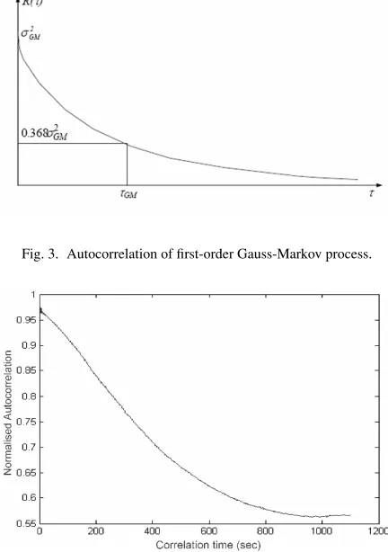
In Fig. 3, the typical autocorrelation function plot of a
first-order Gauss-Markov random process is shown. Figures 4 and 5 describe the normalised autocorrela-tion of the DD ionospheric residuals for the selected satel-lite pairs. Comparing these plots with the typical plot of the autocorrelation of first-order Gauss-Markov processes (Fig. 3), it is reasonable to consider that the DD ionospheric residuals behave asfirst-order Gauss-Markov processes be-cause their autocorrelation functions show a clear exponen-tial attenuation trend similar to that of Fig. 3.
Fig. 3. Autocorrelation offirst-order Gauss-Markov process.
Fig. 4. Normalised autocorrelation of DD ionospheric residuals for satel-lite pair 02-03.
Fig. 5. Normalised autocorrelation of DD ionospheric residuals for satel-lite pair 02-31.
2.3 Kalman filter
A Kalmanfilter algorithm is used to estimate the system state vectorX, which is grouped as follows:
X =
Xp I
i j r m,1 N
i j r m,1 N
i j r m,1−2
T
(11)
The prediction (−) of the state vector at the next epochn+1 is derived from the update (+) of epochnas:
Xn+1(−)=nXn(+)+wn (12)
The parameter Xp in Eq. (11) contains the
W =
Position, velocity and acceleration vectorsXpare expressed
in the local topocentric northing, easting and height coordi-nate system. We ignore any inter-correlation between each component, thus treating each of these as independent of each other. Also, similar to the majority of vehicle motion, the modelling of position and velocity in each dimension (second order system) is considered.
A second-order system equation in one dimension is (Leick, 1995)
The symbolqpdenotes variance of the process noise.
In summary, the state vectorXp, the transition matrixp
and the process noise matrixWpfor a typical dynamic
sys-tem, in the northing, easting, and height coordinate syssys-tem, are easting, and height, respectively, in the geodetic horizon
I =
withqi being the variance of the residual ionosphere
pro-cess noise for the correlation timeτGM.
The DD integer ambiguities are simply modeled as con-stants. The states are transformed into L1integer
ambigui-ties and wide-lane integer ambiguiambigui-ties to take advantage of the longer wide-lane wavelength (86 cm).
2.4 DD ambiguity resolution
To achieve a GPS kinematic position on the centimetre scale, it is necessary to resolve the integer ambiguities in the carrier phase measurements. Float ambiguities are esti-mated as part of the state vector with a Kalmanfiltering al-gorithm. The DD integer ambiguities are modelled as con-stants and are treated as independent from each other.
After an initial transition period and when the estimated integer ambiguities variances reach a predetermined crite-ria, an integer ambiguity search is launched using estimated values as initial guesses. Ambiguities will befixed to inte-gers when the ambiguity search criteria is met.
The search procedure consists in testing all combinations included in a search space and to determine which combi-nation minimises the following quadratic form:
(Nflot−Nent)TCN−1ˆ (Nflot−Nent) (23)
whereNflotis thefloat ambiguities vector,Nentis the integer
ambiguities vector, CNˆ is the float ambiguities
variance-covariance matrix.
To take advantage of the longer wide-lane wavelength (≈86 cm), we first fix the wide-lane integer ambiguities, following which it is relatively easy to determine the L1
integer ambiguities.
3.
Test Results and Analysis
Fig. 6. Averaged post-fit phase residuals.
Table 1. Ionosphere models (processed cases).
Case Ionosphere model
1 N/A
2 White noise
3 Gauss-Markov
4 Random walk
as orbit error and atmospheric effects. For a reliable ambi-guity resolution, the wide-lane combination was used as it enables the number of candidates included in the research space to be reduced, and this combination is less affected (in cycle) by the set of errors affecting the phase measure-ments. In order to reduce the effect of the multipath, as well as the atmospheric effect, we used an elevation mask of 15◦. The small jumps in cycles are practically unavoid-able and are due to the conditions under which the survey was performed (agitated or quiet sea).
In the Kalman filtering method, the dynamic model should be correctly specified. In our study, horizontal co-ordinates are modelled as an integrated velocity, while the average vertical component is modelled as a constant. For differential ionosphere modelling, the autocorrelation anal-ysis of the DD ionospheric residuals, performed previously, shows that ionospheric residuals can be modelled as a first-order Gauss-Markov random process.
Several alternatives have been considered in modelling the correlation time of the ionospheric residuals, including the white noise model (WN), Gauss-Markov process, and the random walk model.
Figure 6 shows the averaged post-fit phase residuals for several data processing cases, which are shown in Table 1. In the first case (N/A), we assume that ionospheric residuals are zero. In the second case (WN), they are modelled as be-ing statistically time independent at each epoch (the correla-tion time is set at zero); the process noise of this WN model was set at 1.0 ppm of the baseline length. In the third case, the temporal behaviour of ionospheric residuals is modelled as a Gauss-Markov process; the correlation time was set at 100 s, the process noise at 0.5 ppm of the baseline length, and the initial uncertainty of the ionosphere at 1.5 ppm of the receiver separation. In the fourth case, we consider a random walk model.
According to Fig. 6, the correlation time value that min-imises the averaged post-fit phase residuals is 100 s.
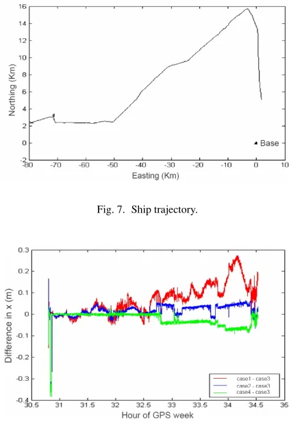
Fig. 7. Ship trajectory.
Fig. 8. Difference in East (x) component.
Fig. 9. Difference in height (z) component.
To quantify the position error induced by bad modelling of the differential ionosphere, the Gauss-Markov model (with 100 s of correlation time) is taken as a reference be-cause residuals are minimum. Rover position coordinates are calculated for the four previous cases. Figure 7 shows the ship’s trajectory; rover positions are determined a 1-s intervals and are expressed in a local topocentric coordinate system for which the reference station is the origin. The observed baselines vary from some hundreds of metres to 80 km.
iono-Fig. 10. PDOP and satellite number.
Fig. 11. Position estimation RMS.
spheric residuals introduces a maximal error of 28 cm in the
xcomponent and 25 cm in thezcomponent. At the begin-ning of observations, differences of about 60 cm correspond to the initial transition period, where ambiguities are not yet resolved.
For distances of about 40 km, the random walk model gives similar results to those obtained for the Gauss-Markov model (with a correlation time of 100 s). This may be discerned from Figs. 8 and 9 where the differences in x
andzfluctuate around zero, until the time tag 32.75 (which corresponds to a baseline of about 40 km).
Figure 10 shows the time behaviour of the geometric dilution of precision (PDOP) and the number of satellites tracked during the surveys; the abrupt changes in the PDOP were caused by the temporary loss of the signal on some satellites. Figure 11 shows the time variation of the esti-mated values of the root mean square (RMS) positions (ob-tained for the Gauss-Markov model with a correlation time of 100 s). As indicated, the RMS has a sharp transition be-tween time tag 30.5 and 31, which indicates that the DD integer ambiguities were determined. The estimated RMS position varies from 3 to 10 cm.
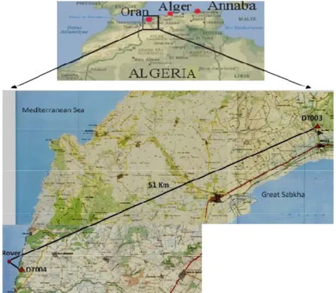
A second set of data recorded (sampling rate 1 s) at a pair of base stations (DT003 and DT004) and with a roving receiver placed on a boat on 13 July 2009 is used. The rover receiver was located a few hundred metres from the DT004 station and about 51 km distant from the DT003 station. Consequently, the data provided both short and long baselines at the same time. Figure 12 shows the location of
Fig. 12. Test data for the comparison between long (DT003 to boat) and short (DT004 to boat) baseline solutions.
the rover and the two base stations.
To validate our approach, we compared the long- and short-baseline solutions. The short-baseline solution is used as reference since the all of the systematic errors, those on the ionospheric effect in particular, are correlated and therefore eliminated by differencing.
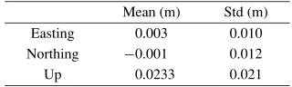
The right side of Fig. 13 shows that the long- (DT003 to boat) and short- (DT004 to boat) baseline solutions differ by only a few centimetres in terms of local geodetic coordi-nates when the ionospheric residuals are estimated. These differences are caused by the presence of the multipath and the tropospheric residuals, which are more significant on the vertical component (about 6 cm for certain epochs). Table 2 summarises the statistics. Mean differences of a few mil-limetres are obtained for the horizontal coordinates and a difference of 2 cm if obtained for the vertical component; the standard deviation (Std; σ) of differences is at a level of 1–2 cm only. Without modelling the ionosphere, dif-ferences may achieve the decimetre level (see left side of Fig. 13).
Figure 14 shows that the ambiguities are fixed after less than 3 min. After the initialisation (fixing ambiguities), the RMS reach the centimetre level.
4.
Conclusion
In the study reported here, we have used the single-reference GPS kinematic positioning method to accurately determine the trajectory of a ship in the water offshore of Oran (Algeria).
In kinematic positioning, the ionospheric effect is the main source of error affecting the integer ambiguity res-olution process and, consequently, the position accuracy. The ionospheric effect becomes increasingly decorrelated as the distance separating the base and the rover receivers increases.
exponen-Fig. 13. Difference between short (DT004 to Boat) and long (DT003 to Boat) baseline solutions in local geodetic coordinates without ionosphere modelling (left) and with ionosphere modelling (right).
Fig. 14. Position estimation RMS.
Table 2. Summary statistics for the difference between short and long baseline solutions.
Mean (m) Std (m)
Easting 0.003 0.010
Northing −0.001 0.012
Up 0.0233 0.021
tial correlation exists between the different adjacent values of ionospheric residuals. These residuals are therefore mod-elled as a Gauss-Markov random process with a correla-tion time of 100 s, which is obtained using an empirical approach, and it concerns all used phase DD. The results of our analysis show that baselines of about 80 km could
be with an accuracy of a few centimetres (based on RMS analysis). The comparison between short- and long- (about 51 km) baseline solutions revealed that mean differences of only a few millimetres and 2 cm were obtained for the hor-izontal coordinates and vertical component, respectively, and that the Std (σ) of differences is at the level of a few centimetres. We note that multipath and troposphere resid-uals are the most significant factors limiting our approach.
Surv. Rev.,37(291), 396–410, 2004.
Coco, D., GPS: Satellites of opportunity for ionosphere monitoring,GPS World,2(9), 47–50, 1991.
Essen, L. and K. D. Froome, The refractive indices and dielectric constants of air and its principal constituents at 24 000 Mc/s,Proc. Phys. Soc., 64(B), 325–356, 1951.
Goad, C. C. and L. Goodman, A modified Hopfield tropospheric refraction correction model, AGU Fall Annual Meeting, San Francisco, CA, USA, 1974.
Han, S. W., Carrier phase-based long-range GPS kinematic positioning, PhD dissertation, rep UNISURV S-49, School of Geomatic Engineer-ing, The University of New South Wales, Sydney, 1997.
Hernandez-Pajares, M., J. M. Juan, and J. Sanz, Application of ionospheric tomography to real-time GPS carrier-phase ambiguities resolution, at scales of 400–1000 km and with high geomagnetic activity,Geophys. Res. Lett.,27(13), 2009–2012, 2000.
Ho, C., Precision orbit determination of Global Positioning System satel-lites,Report CSR-90-2, Center for Space Research, University of Texas, Austin, TX, USA, 1990.
Hopfield, H. S., Two-quartic tropospheric refractivity profile for correcting satellite data,J. Geophys. Res.,74(18), 4487–4499, 1969.
Hu, G. R., H. S. Khoo, P. C. Goh, and C. L. Law, Development and assessment of GPS virtual reference stations for RTK positioning,J. Geod.,77, 292–302, 2003.
Kashani, I., P. Wielgosz, and D. A. Grejner-Brzezinska, The impact of the ionospheric correction latency on long-baseline instantaneous kinematic GPS positioning,Surv. Rev., 2005.
Kim, D. and R. B. Langley, Ionosphere-nullification technique for long-baseline real-time kinematic applications,Navigation. J. Inst. Naviga-tion,54(3), 227–240, 2007.
Klobuchar, J. A., Ionospheric effect on GPS,GPS World,2(4), 48–51, 1991.
Lachapelle, G., P. Alves, L. P. Fortes, M. E. Cannon, and B. Townsend, DGPS RTK positioning using a reference network,Proc 13th Int Tech Meeting Satellite Division US Inst Navigation, Salt Lake City, UT, 19–
22 September, pp 1165–1171, 2000.
Leick, A.,GPS Satellite Surveying, second edition, John Wiley, New York, 1995.
Rothacher, M., Orbits of satellite systems in space geodesy, Ph.D. Disser-tation, Astronomical Institute, University of Berne, Berne, Switzerland, 1992.
Saastamoinen, J., Atmospheric correction for the troposphere and strato-sphere in radio ranging of satellites, inThe Use of Artificial Satellites for Geodesy, Geophysical Monograph No. 15, AGU, Washington, D.C., USA, 1972.
Solheim, F. S., Use of pointed water vapor radiometer observations to im-prove vertical GPS surveying accuracy, Ph.D. Dissertation, Department of Physics, University of Colorado, Boulder, CO, USA, 1993. Vollath, U., A. Buecherl, H. Landau, C. Pagels, and B. Wagner, Multibase
RTK positioning using virtual reference stations,Proceedings of the ION GPS, Salt Lake City, UT, 19–22, pp 123–131, 2000.
Wanninger, L., The performance of virtual reference stations in active geodetic GPS-networks under solar maximum conditions,Proceedings of the ION GPS’99, Nashville, TN, pp 1419–1427, 1999.
Wielgosz, P., D. A. Grejner-Brzezinska, and I. Kashani, Network approach to precise medium range GPS navigation,Navigation,51(3), 213–220, 2004.
Wielgosz, P., I. Kashani, and D. Grejner-Brzezinska, Analysis of long-range network RTK during a severe ionospheric storm,J. Geod.,79, 524–531, 2005.
Wubbena, G., A. Bagge, G. Seeber, V. B¨ oder, and P. Hankemeier, Reduc-¨
ing distance dependent errors for real-time precise DGPS applications by establishing reference station network,Proc 9th Int Tech Meeting Satellite Division US Inst. Navigation, Kansas City, MO, 17–20, pp 1845–1852, 1996.
Yang, M. and C.-F. Lo, Real-time kinematic GPS positioning for centime-ter level ocean surface monitoring,Proc. Natl. Sci, Counc. ROC(A), 24(1), 79–85, 2000.
Zhang, J., Investigations into the estimation of residual tropospheric delays in a GPS network, Master Thesis, UCGE Report 20132, Geomatics Engineering, The University of Calgary, 1999.