Article
Cost-sensitive ensemble feature ranking and
automatic threshold selection for chronic kidney
disease diagnosis
Syed Imran Ali, Bilal Ali, Jamil Hussain, Musarrat Hussain, Fahad Ahmed Satti, Gwang Hoon Park, Sungyoung Lee
Department of Computer Science and Engineering, Kyung Hee University, (Global Campus), 1732, Deogyeong-daero, Giheung-gu, Yongin-si, Gyeonggi-do 17104, Republic of Korea;
[email protected]; [email protected]; [email protected];
[email protected]; [email protected]; [email protected]; [email protected]
Abstract: Automated medical diagnosis is one of the important machine learning applications in the domain of healthcare. In this regard, most of the approaches primarily focus on optimizing the accuracy of classification models. In this research, we argue that unlike general-purpose classification problems, medical applications, such as chronic kidney disease (CKD) diagnosis, require special treatment. In the case of CKD, apart from model performance, other factors such as the cost of data acquisition may also be taken into account to enhance the applicability of the automated diagnosis system. In this research, we have proposed two techniques for cost-sensitive feature ranking. An ensemble of decision tree models is employed in both the techniques for computing the worth of a feature in the CKD dataset. An automatic threshold selection heuristic is also introduced which is based on the intersection of features’ worth and their accumulated cost. A set of experiments are conducted to evaluate the efficacy of the proposed techniques on both tree-based and non-tree tree-based classification models. The proposed approaches are also evaluated against several comparative techniques. Furthermore, it is demonstrated that the proposed techniques select around 1/4th of the original CKD features while reducing the cost by a factor of 7.42 of the original feature set. Based on the extensive experimentation it is concluded that the proposed techniques employing feature-cost interaction heuristic tend to select feature subsets that are both useful and cost-effective.
Keywords: Cost-sensitive feature selection; ensemble models; decision tree classifiers; chronic kidney disease; random forest; gradient boosted trees
1. Introduction
Chronic kidney disease (CKD) is an ailment that affects the functionality of a kidney in the body. Generally, CKD is divided into multiple stages in which the later stages are denoted as a renal failure when the kidney is unable to perform its functions of blood purification and balancing minerals in the body [1]. In the case of end-stage renal failure, hemodialysis is performed to supplant the kidney function. This intervention provides a temporary solution to the problem. Hence, it is of paramount importance that the CKD is detected at earlier stages where it can be addressed through medication and lifestyle changes [2]. CKD is a highly prevalent disease, according to an estimate one in nine Korean adults suffer from kidney disease [3]. Likewise, around 2.5-11.2% of the adult population in Europe also suffer from it, while around 59% of all American adult population is at a high risk of developing kidney disease at some point [4-5]. The high incidence and prevalence of CKD are attributed to its late diagnosis, especially in developing countries [6].
In the domain of medical data mining, several intelligent clinical decision support systems are designed which tend to automate the diagnosis process [6, 42]. These decision systems employ machine learning techniques that assist physicians in the diagnosis and treatment of CKD in an efficient manner [6, 7, 8]. Based on a number of important indicators such as blood pressure, albumin levels, blood and urea tests, potassium, and other comorbidities e.g. diabetes, cardiovascular disease,
etc., a patient is comprehensively assessed for CKD and its progression. As the earlier diagnosis of the disease onset can improve the chances of patients to favorably respond to treatment, therefore, most of the automated systems are optimized for enhancing the overall accuracy of the model [7, 43]. It is noted by Sarah et al [42] that medical decision systems that solely focus on predictive performance are far from the field reality and hence are not unanimously approved by physicians. In this regard, the interpretability of the classification model is stipulated as one of the important requirements among others for a successful medical decision system [42-43]. Similarly, the cost factor as a practicability concern for medical decision systems has recently gained traction in the medical data mining community [6, 16, 40-41]. Therefore, one of the key research directions pursued by the
research community is to design decision systems that are accurate, interpretable, and cost-effective. In a number of studies performed on CKD diagnosis, decision tree models have consistently
produced results with a comparatively higher performance [7, 8, 40]. Hence, the main impetus for using tree-based models in an ensemble technique is two-fold. Firstly, tree models are easy to interpret by the domain experts, therefore in domains such as medical diagnosis, it is desirable to assess the validity of the classification model through visual inspection [37, 42-43]. Secondly, tree-models that are based on bagging and boosting techniques tend to produce highly accurate classifiers on small to medium datasets [7, 6, 8, 23]. Hence, tree models are suitable approaches for considering in an ensemble for a CKD dataset, as they can cater to both types of requirements i.e., interpretability and accuracy.
Moreover, feature selection has become an essential task in building classification models where the objective is to select a subset of useful features [11, 38, 23, 6, 7]. The notion of usefulness is based on the worth of a feature in a dataset in terms of its relevancy and redundancy. There are generally three approaches for feature selection i.e. filter-based approach, wrapper-based approach, and embedded approach [10, 11, 14]. In the case of filter approaches, the worth of a feature is evaluated through univariate statistical approaches such as Chi-Square, Gini index, information gain, etc. Therefore, feature ranking techniques fall into the filter category. On the other hand, wrapper approaches generally, construct a set of candidate feature subsets that are evaluated on a classifier [14]. Embedded techniques are implicitly used by some of the classifiers, such as decision trees while constructing a model.
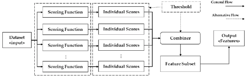
A number of studies have demonstrated that ensemble-based feature selection techniques generally perform better than non-ensemble techniques [7, 11, 12, 13, 38]. Ensemble feature selection approaches are composed of multiple evaluation functions for quantifying the worth of a feature or a subset of features. In this regard, multiple types of feature evaluation functions can be used such as univariate techniques, classification models, or a set of mixed techniques from the aforementioned categories [7]. Ensembles can be comprised of both homogenous and heterogeneous configurations. In this regard, for a homogenous configuration, a dataset is horizontally partitioned into multiple subsets where a single type of the feature evaluation function is executed on each partition [11, 13]. On the other hand, for a heterogeneous configuration, multiple evaluation functions are executed on the dataset in parallel, and later their results are combined [11, 13, 38].
(a) (b)
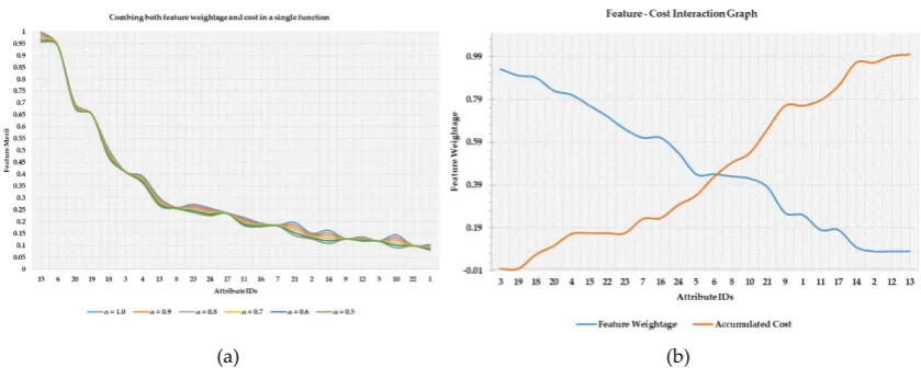
Figure 1. Cost-sensitive feature ranking and threshold selection. (a)Implicit case (b)Explicit case
Most of the studies in the CKD domain assume that the cost of data acquisition is symmetric i.e., having the same cost albeit not necessarily zero; therefore, the cost factor associated with each feature is generally ignored [6, 40, 41]. However, this assumption may not hold in many real-world medical applications where a patient is required to undergo multiple tests such as urine analysis, electrocardiogram, blood culture, etc., and the tests may vary in terms of incurred cost. Therefore, feature selection methods for CKD diagnosis applications may take into account the cost factor as well.
In Figure 1. (a) and (b) a scenario is depicted in which features are listed in descending order of their importance. In Figure 1. (a) a feature merit calculation is performed based on the weightage of a feature and feature’s associated cost. Both these terms are combined using a trade-off constant factor, α, pre-specified by the user. As can be seen in the implicit case that although different ‘α’ values may have the same overall trend it is still not clear which value of a threshold to select among a set of candidate values. Furthermore, after feature number 13, the feature ranking is not consistent with different ‘α’ values. Therefore, the implicit case is not only sensitive to the pre-specified ‘α’, but it also makes it subjective to select a threshold value to retain a set of features. On the other hand, in Figure 1. (b) the blue line denotes feature weightage (FW) while the orange line represents an accumulated cost of selecting a set of features. In the explicit case, a set of features can be easily distinguished at the point of intersection which is comparatively cost-effective and useful than those which are below the intersection point. Hence, in this study, the main question under investigation is this that can the point of feature-cost intersection be used for selecting a subset of features that are both accurate and cost-effective in the CKD diagnosis problem?
Recent studies have reported significant scholarly work on developing chronic kidney disease diagnosis and management systems [6-10, 16-23, 37]. In this regard, this study is in continuation of research performed on the CKD diagnosis problem. The study addresses the problem of cost-sensitive feature selection for building decision tree models for the CKD diagnosis problem. The main objective of the study is to demonstrate that economic considerations can be effectively taken into account along with retaining the overall performance of the CKD diagnosis systems.
into a consolidated feature subset. The multiple feature subsets are combined using the majority voting scheme which is also adopted by several studies [7, 27, 38].
The major contributions of this study are as follows:
• This study demonstrates the application of ensemble-ranking approaches for the cost-sensitive feature selection
• An automatic cost-sensitive threshold selection heuristic is proposed which takes into account both the worth of a set of features along with the accumulated overall cost
• A series of experimentation on benchmarked CKD dataset is performed in order to
demonstrate the effectiveness of our proposed approaches with that of reported approaches on the same dataset over several performance evaluation metrics such accuracy, incurred cost, and number of selected features
• It is also demonstrated that the overall performance and cost-effectiveness of decision tree-based classifiers can be enhanced over CKD diagnosis problem
• The proposed techniques can yield higher average accuracy over non-decision tree models as well for the CKD problem, which shows that the proposed techniques select features with better generalization characteristics
• It is demonstrated that the overall cost of CKD diagnosis can be reduced by a factor of 7.42 through our proposed techniques while reducing the selected feature set to 1/4th of the overall feature set
Figure 2. Schematic diagram of an ensemble feature ranker.
The rest of the paper is organized as follows: Section 2 deals with the literature review on the subject. The proposed methodology is discussed in section 3 in which the proposed ensemble techniques are elaborated. Section 4 deals with the experimentation and the case study results in which we provide a detailed treatment of both the proposed approaches along with their comparison with other related techniques. The conclusion of the study is provided in section 5 along with a set of future directions for extending this research.
2. Literature Review
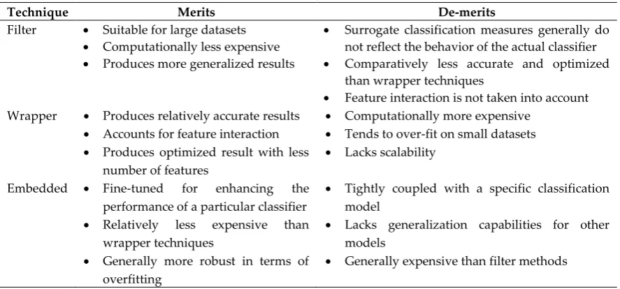
methods are generally employed when the number of features is very large as these methods are computationally fast and do not get bogged down in a pairwise comparison of the candidate feature sets. Wrapper methods generally produce results that are relatively more optimized and accurate than that of the filter methods whereas the latter produces the result in relatively less time [10]. Embedded methods select a subset of features as an integral part of the process of building a classifier such as a decision tree algorithm that selects the most appropriate feature as it grows the tree [15]. A high-level summary (adapted from [39]) regarding the merits and demerits of feature selection techniques is given in Table 1.
Table 1. Comparison among different feature subset selection techniques
Technique Merits De-merits
Filter • Suitable for large datasets
• Computationally less expensive
• Produces more generalized results
• Surrogate classification measures generally do not reflect the behavior of the actual classifier
• Comparatively less accurate and optimized than wrapper techniques
• Feature interaction is not taken into account Wrapper • Produces relatively accurate results
• Accounts for feature interaction
• Produces optimized result with less number of features
• Computationally more expensive
• Tends to over-fit on small datasets
• Lacks scalability
Embedded • Fine-tuned for enhancing the performance of a particular classifier
• Relatively less expensive than wrapper techniques
• Generally more robust in terms of overfitting
• Tightly coupled with a specific classification model
• Lacks generalization capabilities for other models
• Generally expensive than filter methods
reduced CKD dataset. In Ref. [22], the authors experimented with SVM and Artificial Neural Network (ANN) on the CKD dataset. They reported that ANN produced a comparatively higher accuracy model as that of SVM. All the experiments are performed on the top 12 features. Jiongming Qin et al. [23] experimented with several different data imputation configurations on a set of multiple classifiers. They reported that RF achieved the highest accuracy of 99.75% for the CKD diagnosis, while logistic regression (LG) was able to produce an accuracy of 98.95%. Afterward, the authors proposed an integrated model that employed both the aforementioned classifiers along with the perceptron and subsequently produced an accuracy of 99.83% using the integrated approach. Alvaro Sobrindo et al. [6] performed a comprehensive study on CKD diagnosis using various machine learning algorithms. The authors reported the highest accuracy achieved by decision tree-based models in the pool of candidate models which included Naïve Bayes (NB), SVM, ANN, KNN.
We have provided a general overview of the feature selection techniques and classification algorithms applied to CKD diagnosis and it can be observed that decision-tree based models are one of the popular modeling approaches for the CKD diagnosis. Our proposed approach is based on feature ranking therefore we herein mention a few studies which have addressed the problem of automatically selecting an appropriate threshold value using heuristics. Most of the studies opt for a fixed threshold value for retaining a set of top features [24, 25, 26]. But as it is observed that a fixed threshold value may over-select or under-select an appropriate number of features [12, 27, 28, 29]. Authors in [30] used data complexity measures for selecting a threshold value while [31] used a minimum union method to combine multiple rankings and produced promising results on high dimensional datasets [32]. Chih-Fong Tsai and Yu-Chieh Hsiao [38] performed a detailed study regarding combining multiple feature selection methods for stock prediction problem. The authors reported higher predictive accuracy over the ANN classifier based on the multi-point interaction among Principal Component Analysis (PCA) and Genetic Algorithm (GA) and Decision Tree (DT) feature sets, among other combination strategies. Opeyemi Osanaiye et al. [46] proposed an ensemble feature selection technique in which the authors combine partial results from multiple filter measures. Subsequently, 1/3rd features from each feature selection method are retained. A Consolidated feature subset is obtained through the intersection of the candidate feature subsets.
Although a number of threshold selection approaches are reported in the literature that is primarily geared towards optimizing the accuracy of the classification task. But the aforementioned approaches cannot take into account valuable meta-information associated with the feature set, such as cost of data acquisition. It is important to note that the cost-free feature selection approaches may also result in cost reduction (c.f. Table 11) but such a cost reduction results would be effectively unintentional since the cost-free feature selection methods are oblivion to the cost meta-data associated with the features. Our proposed approaches are based on explicitly taking into account the cost factor along with the feature worth. In this regard, we show that an automatic threshold value can be selected based on the feature-cost interaction curve, as shown in Figure 1. (b), which results in a feature set that is both useful and cost-effective. In the following section, we elaborate on the proposed methodology for computing feature weightage along with the application of a threshold value in arriving at a final feature set.
3. Proposed Methodology
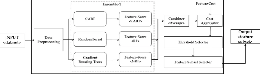
collectively, they enhance the overall model’s performance. In this regard, the feature ranking approach depends on the comprehensiveness of the weighting function. Therefore, in this research, we have used three decision-tree based classification models, Classification and Regression Tree (CART), RF and, Gradient Boosting Trees (GBT), which evaluate both the relevance and redundancy of a feature set. It is important to note that the model-based scoring functions can be executed in parallel, therefore the running time of the ensemble is proportional to the running time of its slowest classifier. In this regard, using concurrent processes we can execute the classifiers and afterward combine their results. The main objective of the feature weightage step is to score features based on their importance as well as their interaction with other features in the dataset. Once a reliable feature score is obtained, based on their weightage, features are ranked in descending order of their importance. Subsequently, an averaging operation is performed on the obtained feature weightage and a final feature score is generated.
In this research, we propose two approaches for combining features i.e. ensemble-1 is based on combining individual scores, whereas ensemble-2 generates three partial solutions in the form of three subsets obtained from the scoring functions. Afterward, the partial solutions are combined using the majority vote. In ensemble-1, a threshold value based on the feature-cost intersection is selected after combining multiple lists, whereas, in ensemble-2 the threshold is applied on an individual list which is obtained from the scoring function and a resultant feature subset is generated. Each feature subset is treated as a partial solution. A final solution is obtained by applying the majority vote scheme to the partial solutions. We have normalized the cost values; hence the overall cost of the entire feature set adds-up to 1. The proposed ensemble-1 is depicted in Figure 3, while Figure 4 shows ensemble-2.
Figure 3. Thearchitecture of the proposed ensemble-1.
Figure 4. Thearchitecture for the proposed ensemble-2.
3.1. Data Preprocessing
which are similar to the missing value record and subsequently imputes the missing value based on the local information of the selected instances. Furthermore, we used Euclidean distance for computing the similarity of numerical attributes. Numerical values are replaced with taking the mean value of the selected attribute while mode value is used for nominal features. The chronic kidney disease dataset, discussed in the subsequent section, contains 242 records with missing values while the complete dataset has 400 records. Therefore, around 60% of the records have one or more missing values.
3.2. Classifier-Ensemble
The proposed approach uses a decision tree-based classifiers. Following is a brief description of the classification models used in the ensemble:
Classification and Regression Tree: It is one of the popular decision tree induction algorithms. CART creates strictly binary decision trees by employing recursive partitioning to build the model [45]. CART selects a subset of features from the complete feature set for building a decision tree model. The choice of feature selection is based on the quantification of a feature’s worth in generating a homogenous data subset. Generally, the Gini index is used to calculate the importance of a feature at a specific level in the tree whereas information gain is also one of the popular choices for feature quantification. The main objective of the CART algorithm is to construct the model which can separate the data into homogenous subsets with respect to the class label. We have used the Gini index to calculate the impurity of a feature subset. Feature weightage is obtained from CART by taking into account the effect of adding a feature to the decision tree and the subsequent decrease in the impurity in the model.
Random Forest: It is based on a decision tree model where a set of decision trees are generated. In this case, each tree is incrementally improved by partitioning the dataset into homogenous subsets [40]. RF creates a set of pre-defined decision trees where each tree is constructed from a bootstrapped dataset. RF generally performs well for small to medium-sized datasets and the resulting model is robust against overfitting, feature interaction, and spurious data patterns [34]. The key approach of this algorithm is to create a set of bootstrapped datasets through which a set of pre-defined randomly selected features are selected and a tree model is created. The standard RF model is a combination of binary decision trees. Unlike CART, RF is an ensemble tree model where multiple decision trees are created for introducing diversity in the overall model. Bagging is applied to the input dataset through which several data subsets are created. Generally, trees are constructed based on randomly selected features but other feature selection schemes can also be used [40]. Finally, all the generated trees are integrated through a majority voting scheme for the classification problem. Although the resulting model is not fully interpretable as that of CART, the individual decision trees can be extracted. Similarly, feature weightage is computed by taking into account the average decrease in impurity over all the trees in an ensemble.
Gradient Boosted Trees: It is an ensemble modeling technique for either regression or classification problems. It is based on a forward-learning approach in which predictive results are incrementally improved through introducing weak models. A weak model is one that is slightly better than a random guess. GBT is based on a non-linear regression procedure that improves the accuracy of decision trees. Weak classification tree models are applied to different distributions of the dataset in a sequential manner where misclassified data points are given higher weightage. As weak models are added to the integrated model the error recorded through the loss function minimizes by applying the gradient descent approach. In the case of GBT, the feature weightage can be obtained by the sum of improvements for a given attribute at a node.
3.3. Combiner
It plays an important role in the overall proposed architecture.
feature weightages into a consolidated score. The final scores are obtained by taking the average across multiple scoring functions as shown in equation (3):
𝑓= 1
|𝑠| ∑ 𝜎𝑖(𝑓)
𝑠
𝑖=1 (1)
The final score of a given feature ‘𝑓̂’ is the average weightage across three independent scoring functions ‘σ’applied on a feature ‘𝑓’, where ‘s’ is the total number of functions in the ensemble. Please note that the scoring values are scaled between 0 and 1 before applying equation 3.
Algorithm 1 Ensemble -1
Input: Dataset D, Cost vector Cv
Output: Selected feature set S
N: number of scoring functions in ensemble
1: Begin
2: foreach m in N do:
3: score[m] = score_function(m, D)
4: endfor
5: L = average (score [1: N]) // using equation (3)
6: *L = sort(L) // *L, is sorted in descending order
7: foreach f in *L do:
8: Cscore [] = f-1cost + cost(f, Cv) //cost accumulation for current and previous features
9: endfor
10: T = intersection (*L, Cscore[]) // where FW < Cscore, and FW = *L.score;
11: S = retained (*L, T) // retained features in *L after applying T
12: return S
13: End
• Ensemble-2 deals with multiple partial solutions in the form of feature subsets. In this case, each scoring function produces an independent ranked list. A threshold operation is applied to each list. Subsequently, three different subsets are produced. All the subsets are combined by taking the majority voting scheme. In our case, as the ensemble is comprised of 3 scoring functions, therefore the majority voting is effectively translated into the selection of a feature that is present into at least 2/3rd of the subsets.
Algorithm 2 Ensemble -2
Input: Dataset D, Cost vector Cv
Output: Selected feature set S
N: number of scoring functions in ensemble
1: Begin
2: foreach m in N do:
3: score[m] = score_function(m, D) //m: DT, RF, GBT
5: foreach f in *L do:
6: Cscore [] = f-1cost + cost(f, Cv) //cost is calculated
for each evaluation function
7: endfor
8: T = intersection (*L, Cscore[])
9: Sm = retained (*L, T)
10: endfor
11: S = combine(𝑆1, 𝑆2, 𝑆3) //using majority vote scheme
12: return S
13: End
3.4. Feature cost aggregator
Feature cost aggregator is used for selecting a threshold value over a feature weightage curve. Both ensemble-1 and ensemble-2 approaches use a threshold to select a subset of features. Features are arranged in the descending order of their combined score. The individual cost of a feature is retrieved and accumulated in a top-down manner as given in equation 4.
𝐶𝑜𝑠𝑡(𝐹𝑖) = 𝐶𝑜𝑠𝑡 (𝐹𝑖) + 𝐶𝑜𝑠𝑡 (𝐹𝑖−1) (2)
Where i = 1, 2, 3, …, m. Therefore, Cost(F0) = 0
In this study, values of the cost feature are normalized between 0 and 1. Please note that although the feature score curve is calculated only once, whereas, different cost factors associated with a feature may generate different accumulated cost (C-score) curves. In this study, we have investigated the
economic cost perspective, whereas other cost factors such as data’s availability, risk, the computational cost may also be taken into account.
3.5. Threshold and Feature Subset Selector
The purpose of the threshold value is to select a subset of features from the given feature list after incorporating the cost value. Ensemble-1 produces a feature list based on average scores. In this regard, we can find a point of intersection between feature weightage and the corresponding accumulated cost values. The point of intersection between ‘FW’and accumulated cost score ‘C-score’ can be found where 𝐹𝑊 < 𝐶𝑠𝑐𝑜𝑟𝑒. A sample graph based on the feature-cost intersection curve is depicted in Figure 1. (b). A threshold value is automatically selected based on the point of intersection e.g. point of intersection is at feature number 6 in Figure 1. (b). Hence, all the features starting from feature number 3 leading up to feature number 6 would be retained while the rest of the features would be discarded. The assumption taken in this regard is that the features over the interaction point are reasonably useful and cost-effective, whereas, the accumulated cost of features below the intersection point out-weight their importance.
ensemble. As we have three classifiers, therefore, the highest score a feature may get is 3. In Table 2, the selected features are denoted with boldface letters while the remaining features are discarded.
It is important to note that the subsets generated by scoring functions may not be of equal size. Since for each scoring function e.g. CART, features’ weightage are obtained and then subsequently based on the intersection of the FW and the accumulated cost i.e. C-score, similar to the ensemble-1 approach, a subset of features is selected for each function. More details regarding this step are presented in the experimentation section.
Table 2. Ensemble-2 frequency-based feature ranking.
Subset 1 Subset 2 Subset 3 Feature ID Frequency
3 19 3 3 3
6 18 19 19 3
20 3 20 18 3
19 15 4 20 2
7 5 22 4 2
16 8 18 15 2
22 14 23 22 2
18 2 12 23 2
4 1 21 7 1
23 9 11 16 1
… … … … …
4. Experimentation
This section deals with the experimentation details of the study. In this regard, a brief description of the dataset is provided along with a summarized analysis of the quality of the dataset. Afterward, we elaborate on the performance metrics used in this study and the interpretation of the results. Furthermore, we carry on two sets of experiments. Experiment 1 deals with evaluating the efficacy of ensemble-1 with that of the baseline models, while ensemble-2 is compared with baseline models in experiment 2. Once, we establish the performance of both the proposed approaches, we then compare them with other similar methods mentioned in section 2, over several performance metrics and incurred cost.
To demonstrate the efficacy and applicability of our proposed approach, we have used a benchmark dataset from the University of California (UCI) online repository [35]. The chronic kidney disease (CKD) is a real-world dataset acquired over a period of two months by Apollo Hospitals, Tamilnadu, India.
4.1. Dataset description
The CKD dataset is composed of 400 instances where each instance is comprised of 24 attributes excluding the class attribute. There are 13 categorical attributes while 11 of the attributes have numerical values. The dataset is used to model a dichotomous decision variable i.e. 1 represents a given patient is diagnosed with the disease, while -1 denotes otherwise. The overall dataset has 250 CKD patients while the rest of the patients have a non-CKD diagnosis. The acquired data are preprocessed to impute missing values and ID attributes. Table 3 provides a summary of the CKD dataset, along with the economic cost of acquiring data for a particular feature. The cost factor associated with each attribute is adopted from Asif Salekin and John Stankovic [16].
Table 3. Chronic Kidney Disease dataset description.
ID Attribute Cost Description ID Attribute Cost Description
1 Age <age:
numerical> 1 In years 13
Sodium <sod:
2 Blood Pressure <bp:
numerical> 1 Mm/Hg 14
Potassium <pot:
numerical> 50 mEq/L
3 Specific Gravity <sg: numerical> 1
1.005, 1.010, 1.015, 1.020,
1.025
15 Hemoglobin <hemo:
numerical> 2.65 Gms
4 Albumin <al:
numerical> 26 0 ~ 5 16
Packed Cell Volume <pcv: numerical> 2.62
Integer valued
5 Sugar <su:
categorical> 21 0 ~ 5 17
White Blood Cells Count <wc: numerical>
31 cells/cumm
6 Red Blood Cells
<rbc: categorical> 40
1:Normal,
0:Abnormal 18
Red Blood Cells Count <rc: numerical>
31 millions/cmm
7 Pus Cell <pc:
categorical> 31
1:Normal,
0:Abnormal 19
Hypertension <htn:
categorical> 1 1:Yes, 0:No
8 Pus Cell Clumps <pcc: categorical> 31
1:Present,
0:Absent 20
Diabetes Mellitus
<dm: categorical> 19.4 1:Yes, 0:No
9 Bacteria <ba:
categorical> 51
1:Present,
0:Absent 21
Coronary Artery Disease <cad:
categorical>
51 1:Yes, 0:No
10
Blood Glucose Random <bgr: numerical>
21 mgs/dl 22 Appetite <appet:
categorical> 1
1:Good, 0:Poor
11 Blood Urea <bu:
numerical> 12.85 mgs/dl 23
Pedal Edema <pe:
categorical> 1 1:Yes, 0:No
12 Serum Creatinine
<sc: numerical> 15 mgs/dl 24
Anemia <ane:
categorical> 28.64 1:Yes, 0:No
The attribute importance in terms of its correlation with the class variable is shown in Figure 6. As it can be seen that several features have a high correlation with the target concept. The nature of correlated features and their treatment are generally domain-dependent and therefore, a decision-maker is generally involved to decide on either retaining or removing highly correlated features. In the absence of a domain expert, features having higher correlation are generally preferred over lower correlation features but in the case where the availability of such features is not certain at the time of decision making then it is recommended to remove such highly correlated features.
Figure 6. Pareto-chart of features in the CKD dataset.
4.2. Experimental setup
tree-based models as well as other well-known classification algorithms. Moreover, extensive experimentation is also performed in which a number of relevant techniques are compared with that of the proposed approaches. All of the experiments are performed on a system having processor AMD Ryzen 3 2200G with 8 GB RAM and 64-bit Windows 10 Enterprise Edition. In this study, we have used the RapidMiner Studio 9.6 version [36] for simulating the proposed approaches. Workflows related to generating feature weightage for different feature scoring functions are hosted at MyExperiment.org which is a collaborative repository to share workflows and other associated files [48-50].
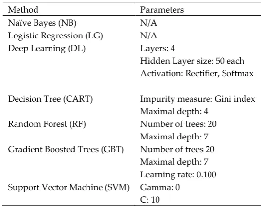
Table 4. Classification models parameters
Method Parameters
Naïve Bayes (NB) N/A
Logistic Regression (LG) N/A Deep Learning (DL) Layers: 4
Hidden Layer size: 50 each Activation: Rectifier, Softmax
Decision Tree (CART) Impurity measure: Gini index Maximal depth: 4
Random Forest (RF) Number of trees: 20 Maximal depth: 7 Gradient Boosted Trees (GBT) Number of trees 20
Maximal depth: 7 Learning rate: 0.100 Support Vector Machine (SVM) Gamma: 0
C: 10
Table 2 shows the parameters selected against each classification model. To evaluate the efficacy of the proposed approaches, we have used several evaluation metrics such as accuracy, precision, recall also known as sensitivity, specificity, F1-measure, and Area under Receiver Operating Characteristics Curve (AUC). The evaluation metrics are computed through the confusion matrix, such as:
True Positive (TP): denotes positive instances predicted as positive True Negative (TN): denotes negative instances predicted as negative False Positive (FP): denotes negative instances predicted as positive False Negative (FN): denotes positive instances predicted as negative
Based on the aforementioned definitions, the quality metrics of interest are calculated as follows:
Accuracy = 𝑇𝑃 + 𝑇𝑁 𝑇𝑃 + 𝐹𝑃 + 𝑇𝑁 + 𝐹𝑁
(1)
𝑃𝑟𝑒𝑐𝑖𝑠𝑖𝑜𝑛 = 𝑇𝑃 𝑇𝑃 + 𝐹𝑃
(2)
𝑅𝑒𝑐𝑎𝑙𝑙/𝑆𝑒𝑛𝑠𝑖𝑡𝑖𝑣𝑖𝑡𝑦 = 𝑇𝑃
𝑇𝑃 + 𝐹𝑁
(3)
𝑆𝑝𝑒𝑐𝑖𝑓𝑖𝑐𝑖𝑡𝑦 = 𝑇𝑁
𝑇𝑁 + 𝐹𝑃 (4)
𝐹1 − 𝑚𝑒𝑎𝑠𝑢𝑟𝑒 = 2 ∗ (𝑅𝑒𝑐𝑎𝑙𝑙 ∗ 𝑃𝑟𝑒𝑐𝑖𝑠𝑖𝑜𝑛) (𝑅𝑒𝑐𝑎𝑙𝑙 + 𝑃𝑟𝑒𝑐𝑠𝑖𝑜𝑛)
(5)
classification models. In this manner, the reported result values for each classification model are averaged over different testing partitions.
5. Results and analysis
5.1. Baseline Results
In this section, we report the results of the baseline models over the full CKD dataset without any feature selection as shown in Table 5.
Table 5. Evaluation results for baseline models.
Models Accuracy Precision Recall Specificity F-measure AUC Cost
NB 62.3 ± 2.0 % 62.3 ± 2.0% 100.0 ± 0.0 0.0 ± 0.0% 76.6 ± 1.5 % 0.908 ± 0.09
475.36
LG 84.3 ± 6.6% 83.2 ± 5.8% 94.3 ± 9.3% 66.9 ± 14.0% 88.2 ± 5.6% 0.952 ± 0.58
DL 89.5 ± 2.3% 85.4 ± 2.8% 100.0 ± 0.0% 72.8 ± 5.7% 92.1 ± 1.6% 1.0 ± 0.0
DT 87.7 ± 4.8% 97.3 ± 3.7% 90.4 ± 10.5% 95.6 ± 6.1% 93.3 ± 4.5% 0.966 ± 0.03
RF 89.5 ± 3.5% 83.9 ± 3.6% 100.0 ± 0.0% 66.4 ± 11% 91.2 ± 2.2% 0.998 ± 0.004
GBT 73.8 ± 5.8% 86.2 ± 6.9% 100.0 ± 0.0% 71.4 ± 15.6% 92.5 ± 4.0% 1.0 ± 0.0
SVM 92.2 ± 9.0% 71.8 ± 8.1% 97.2 ± 3.8% 35.8 ± 20.7% 82.4 ± 5.6% 0.844 ± 0.12
Average 82.75 ± 4.8% 81.44 ± 4.7% 97.41 ± 3.3% 58.41 ± 10.4% 88.07 ± 3.5% 0.952 ± 0.04
5.2. Feature weightage calculation and feature subset acquisition
As mentioned earlier, both ensemble-1 and ensemble-2 approaches require a robust feature scoring function. In this regard, three decision tree-based classifiers are used as the scoring functions to obtain a consolidated feature score. In the following section, we elaborate on the feature scores obtained from different functions along with the feature subsets selected. Please note, that ensemble-1 combines individual weightage obtained from multiple scoring functions and afterward selects a threshold, whereas, ensemble-2 is based on an eager approach in which threshold is applied to individual scoring functions and a set of feature subsets are obtained which are afterward combined into a consolidated feature set.
• Decision Tree Score: Features are scored through the CART decision tree classifier. The blue line shows the feature weightage (FW) in the decreasing order of their importance while the orange line denotes accumulated cost (C-score). Both the values are normalized. The point of intersection between FW and C-score is found around feature number 5 as shown in Figure 7.
• Random Forest Score: The second scoring function is based on random forest. The blue line shows the feature weightage (FW) while the orange line denotes accumulated cost (score). Both the values are normalized. The point of intersection between FW and C-score can be observed around feature number 9 as shown in Figure 8.
Figure 8. Random forest-based feature scoring.
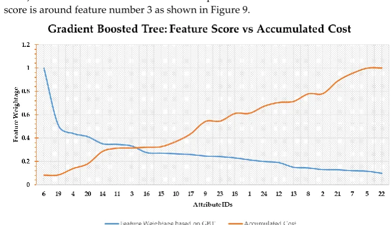
• Gradient Boosted Trees Score: The last scoring function is based on GBT. The blue line shows the feature weightage (FW) while the orange line denotes accumulated cost (score). Both the values are normalized. The point of intersection between FW and C-score is around feature number 3 as shown in Figure 9.
Figure 9. Gradient boosted trees based feature scoring.
In this study, all the feature scoring functions are based on decision tree family models. Therefore, it would be interesting to investigate the correlation of generated ranking lists. We have used the Kendall rank correlation coefficient [47] to compute the pair-wise correlation of lists produced by DT, RF, GBT as shown in Table 6.
Table 6. Kendall rank correlation coefficient for different scoring functions
-0.17 -0.09 0.22
As it can be observed that the correlation between different lists is closer to zero. The correlation results of the ranked lists support the null hypothesis of mutual independence. Therefore, we can conclude that there is statistically significant independence between the ranked lists. Furthermore, the lists generated by both GBT and DT are relatively in agreement with each other while the lists produced by DT and RF, and RF and GBT show disagreement. In this regard, each scoring function is accounting for important characteristics of the dataset while not diverging too much in their final results.
Furthermore, we can also look at different feature subsets obtained from the aforementioned scoring functions (ref. Table 7) and their Jaccard index value. Figure 10 depicts a Venn diagram for all possible logical relations among different feature subsets.
Figure 10. Jaccard index of different feature subsets
It is interesting to note that although the ranked lists produced by GBT and DT have a higher correlation, whereas, the feature subsets obtained after applying a threshold value to the respective lists have a lower value on the Jaccard index i.e. 0.1000. On the other hand, a higher Jaccard index value is obtained between RF and GBT feature subsets while their ranked lists reported a negative correlation (ref. Table 6). Based on these observations we can conclude that both the lists and the subsequent feature subsets obtained from the scoring functions are not redundant.
The resulting selected features collected in list 1, list 2, and list 3 are based on the decision tree, random forest and gradient boosted trees, respectively. As it can be seen that there are some variations in the selected features which shows that each scoring function has its own inductive bias while constructing a model as shown in Table 7. A detailed study of the inductive bias of decision tree models is not within the scope of this study.
Table 7. Selected features by individual scoring functions.
Scoring function List Selected features
Decision Tree L1 15, 6, 17, 24, 5. Random Forest L2 20, 19, 18, 6, 15, 3, 22, 9 Gradient Boosted Trees L3 6, 19, 4, 20, 14, 11, 3
The averaged evaluation results of the aforementioned seven classification models are provided in Table 8. These results reflect the performance of classification models on reduced datasets acquired from each scoring function (ref. Table 7). In this regard, the decision tree classifier is constructed based on features present in list L1. Likewise, classifiers for random forest and gradient boosted trees are built on L2 and L3, respectively.
Scoring Function
Average Accuracy
Average Precision
Average Recall
Average Specificity
Average F-measure
Average AUC
Cost
DT Only 71.95 ± 3.44% 70.21 ± 2.94% 99.01 ± 1.28% 27.32 ± 7.05% 81.78 ± 2.27% 0.937 ±0.056 123.29
RF Only 96.01 ± 2.64% 95.30 ± 2.71% 98.78 ± 1.91% 90.42 ± 5.92% 96.98 ± 2.25% 0.995 ± 0.006 197.05
GBT Only 85.24 ± 3.88% 84.71 ± 4.58% 98.34 ± 2.14% 63.22 ± 13.18% 90.25 ± 3.01% 0.941 ± 0.05 150.25
The overall performance of the random forest and gradient boosted trees have increased (ref. Table 5 and Table 8). Although the decision tree could not improve the accuracy over the full dataset, it has slightly improved the sensitivity. As it can be seen that the automatic threshold selection has successfully opted for threshold values which resulted in the selection of important features while also keeping the overall cost of the selected feature set low. Hence, the feature subsets produced by different scoring functions are both relevant in enhancing the accuracy of the classification models and distinct.
5.3. Ensemble-1 Results
Feature weightage obtained from individual scoring functions are consolidated through an averaging operation. The intuition behind the consolidation process is that the final scores will reflect both low-cost and high-accuracy characteristics of the individual functions. Figure 11 shows the feature-cost interaction graph for ensemble 1.
Figure 11. Ensemble-1 based feature scoring.
As can be seen in Figure 11 that the point of intersection is around feature number 3. Therefore, all the features starting from number 6 up to number 3 i.e. 6, 15, 20, 19, 18, and 3, would be selected. In this regard, Table 9 shows the results of evaluation metrics for features selected by the ensemble-1 approach.
Table 9. Ensemble-1 results based on selected features.
Models Accuracy Precision Recall Specificity F-measure AUC Cost
NB 98.25 ± 2.92% 95.72 ± 3.81% 98.78 ± 1.64% 91.94 ± 7.55% 97.14 ± 2.21% 0.995 ± 0.006
95.05
LG 99.10 ± 1.90% 98.80 ± 2.80% 100.0 ± 0.0% 97.50 ± 5.60% 99.40 ± 1.40% 1.0 ± 0.0
DL 97.40 ± 2.40% 96.10 ± 3.60% 100.0 ± 0.0% 93.10 ± 6.40% 98.0 ± 1.90% 1.0 ± 0.0
DT 89.40 ± 4.0% 87.70 ± 5.20% 97.10 ± 3.90% 76.40 ± 12.3% 92.10 ± 2.80% 0.975 ± 0.03
RF 98.30 ± 2.4% 97.50 ± 3.4% 100.0 ± 0.0% 95.0 ± 6.805 98.70 ± 1.80% 1.0 ± 0.0
GBT 95.70 ± 4.3% 93.80 ±6.1 % 100 ± 0.0% 88.30 ± 11.9% 96.70 ± 3.20% 1.0 ± 0.0
SVM 95.60 ± 3.1% 96.20 ±5.6 % 97.20 ± 3.8% 93.30 ± 9.90% 96.50 ± 2.40% 0.993 ± 0.009
A cursory glance at Table 8 and Table 9 shows that the proposed ensemble-1 technique has successfully reduced the overall cost while improving the key evaluation metrics over the individual scoring functions. Moreover, multiple combinations of feature scoring functions and their respective averaged results over seven classification models are shown in Table 10.
Table 10. Multiple combinations of scoring functions and their respective results Scoring
Functions
Averaged Accuracy
Averaged Precision
Averaged Recall
Averaged Specificity
Averaged F-measure
Averaged
AUC Cost
DT Only 71.95 ± 3.44% 70.21 ± 2.94% 99.01 ± 1.28% 27.32 ± 7.05% 81.78 ± 2.27% 0.937 ±0.056 123.29
RF Only 96.01 ± 2.64% 95.30 ± 2.71% 98.78 ± 1.91% 90.42 ± 5.92% 96.98 ± 2.25% 0.995 ± 0.006 197.05
GBT Only 85.24 ± 3.88% 84.71 ± 4.58% 98.34 ± 2.14% 63.22 ± 13.18% 90.25 ± 3.01% 0.941 ± 0.05 150.25
DT-RF 93.78 ± 3.04% 95.29 ± 4.90% 95.31 ± 6.50% 91.41 ± 9.00% 95.04 ± 2.57% 0.99 ± 0.02 143.69
DT-GBT 91.40 ± 2.27% 91.89 ± 3.01% 96.01 ± 4.36% 83.79 ± 5.61% 93.59 ± 1.89% 0.95 ± 0.02 162.54
GBT-RF 93.39 ± 2.70% 91.53 ± 4.07% 99.19 ± 1.47% 83.80 ± 8.19% 95.04 ± 1.96% 1.00 ± 0.01 172.05
Ensemble-1 96.26 ± 2.93% 95.73 ± 3.81% 98.79 ± 1.64% 91.94 ± 7.56% 97.14 ± 2.21% 1.00 ± 0.01 95.05
5.4. Ensemble-2 Results
As mentioned earlier in section 3.5, the ensemble-2 is based on consolidating the feature subset acquired from different scoring functions in such a manner that the majority of the features are retained from the individual subsets while the rest of the features are discarded. Table 11 shows features subsets acquired from different scoring functions and the final consolidated solution based on the ensemble-2 technique.
Table 11. Feature selected through ensemble-2.
Scoring function List Selected features Frequency
Decision Tree L1 15, 6, 17, 24, 5.
6:3, 3:2, 15:2, 19:2, 20:2, 1:1, 2:1, 4:1, 5:1, …
Random Forest L2 20, 19, 18, 6, 15, 3, 22, 9 Gradient Boosted Trees L3 6, 19, 4, 20, 14, 11, 3
Ensemble-2 *L 6, 15, 20, 19, 3
In this regard, Table 12 shows the evaluation metrics applied to the classification models constructed from the ensemble-2 feature subset.
Table 12. Ensemble-2 results based on selected features.
Models Accuracy Precision Recall Specificity F-measure AUC Cost
NB 96.5 ± 3.60% 100.0 ± 0.0% 94.40 ± 6.0% 100.0 ± 0.0% 97.0 ± 3.20% 1.0 ± 0.0
64.05
LG 96.5 ± 2.0% 100.0 ± 0.0% 94.50 ± 3.10% 100.0 ± 0.0% 97.10 ± 1.60% 0.997 ± 0.007
DL 100.0 ± 0.0% 100.0 ± 0.0% 100.0 ± 0.0% 100.0 ± 0.0% 100.0 ± 0.0% 1.0 ± 0.0
DT 93.90 ± 6.60% 100.0 ± 0.0% 90.40 ±10.50% 100.0 ± 0.0% 94.70± 5.9% 0.952 ± 0.052
RF 98.30 ± 2.40% 97.40± 3.50% 100.0 ± 0.0% 95.30 ± 1.80% 98.70 ± 1.8% 0.998 ± 0.004
GBT 100.0± 0.0% 100.0 ± 0.0% 100.0 ± 0.0% 100.0 ± 0.0% 100.0 ± 0.0% 1.0 ± 0.0
SVM 95.70 ± 4.30% 98.70 ± 3.0% 94.50 ± 7.60% 97.80 ± 5.0% 96.30 ± 3.70% 0.961 ± 0.057
Average 97.27 ± 2.92% 99.44± 0.92% 96.25 ± 3.88% 99.01 ± 1.64% 97.68 ± 2.31% 0.986 ± 0.017
Table 13. Multiple combinations of scoring functions and their respective results
Case Averaged
Accuracy
Averaged Precision
Averaged Recall
Averaged Specificity
Averaged F-measure
Averaged
AUC Cost
Intersection 62.30 ± 2.0% 62.30 ± 2.0% 100.0 ± 0.0% 0.0 ± 0.0% 76.80 ± 1.50% 0.56 ± 0.03 31
Union 89.77 ± 2.43 % 89.56 ± 2.99 % 97.61±3.01 % 76.96 ± 6.94% 92.77 ± 1.81% 0.98 ± 0.01 317.54
Multi-
intersection 97.27 ± 2.70% 99.44 ± 0.93% 96.26 ± 3.89% 99.01 ± 1.64% 97.69 ± 2.31% 0.99 ± 0.02 64.05
In terms of comparative analysis between ensemble-1 and ensemble-2 (ref. Table 9 and Table 12), it can be observed that for the CKD problem the latter performs better in terms of accuracy, precision, specificity, F1-measure, the cardinality of selected features and the overall cost of the solution. It would be interesting to explore whether these results generalize to other cost-sensitive diagnosis problems or not?
5.5. Comparison with other similar approaches
In this section, we compare our results with other feature selection approaches on the CKD dataset. All the experiments are performed on the aforementioned seven classifiers, and subsequently, the averaged results are reported in Table 14.
Table 14. Multiple combinations of scoring functions and their respective results
Method Averaged
Accuracy
Averaged Precision
Averaged Recall
Averaged Specificity
Averaged F-measure
Averaged
AUC Cost
[7] 83.29±5.07% 82.65±5.82% 97.20±3.34% 60.04±12.11% 88.55±3.75% 0.934±0.50 167.31
[9] 93.41±3.27% 94.24±3.04% 96.61±3.34% 88.20±6.21% 95.0±2.64% 0.981±0.02 272.20
[10] 85.74±2.44% 84.92±2.91% 99.40±1.0% 62.94±4.84% 90.75±1.82% 0.918±0.02 236.11
[23] 92.64±2.74% 93.5±2.45% 97.38±3.02% 84.68±5.44% 94.41±2.15% 0.987±0.01 141.10
[24] 87.37±3.40% 86.84±3.47% 98.62±1.50% 68.87±9.18% 92.95±2.42% 0.976±0.03 136.72
[38] 90.0±2.80% 90.71±2.57% 97.22±2.60% 78.25±4.31% 93.07±2.22% 0.979±0.02 193.70
[46] 90.51±3.24% 89.54±4.18% 98.6±1.80% 80.60±8.20% 93.31±2.42% 0.994±0.02 91
Ensemble-1 96.26±2.92% 95.72±3.81% 98.76±1.64% 91.94±7.55% 97.14±2.21% 0.995±1.0 95.05
Ensemble-2 97.27±2.70% 99.44±0.82% 96.25±3.88% 99.01±1.64% 97.68±2.31% 0.986±4.0 64.05
A detailed comparison based on similar techniques and proposed techniques is drawn in Table 14. The boldface values denote the best performance achieved under a specific criterion. As it can be seen that most of the comparative techniques are primarily optimized to produce models with higher accuracy. Therefore, in terms of accuracy, the difference between the competing approaches is not much pronounced. But it can be noted that ensemble-2 produces a highly cost-effective and accurate solution for the CKD diagnosis problem within the purview of similar approaches experimented in this study.
Figure 12. Combined ranks of different approaches across performance and cost factors
6. Conclusion
Cost-sensitive feature selection is one of the important areas of research where the cost of data acquisition plays an important role in the applicability of the solution. Generally, it is assumed that cost of data acquisition is the same i.e. not necessarily zero. This assumption does not hold in certain application domains such as disease diagnosis. In this study, we have used a well-known benchmarked dataset for disease diagnosis i.e. chronic kidney disease. A significant scholarly work is reported in designing algorithms and systems for chronic kidney disease efficiently. The proposed techniques for cost-sensitive feature selection reported in this study is in the continuation of CKD research, where the key objective is to enhance the performance of decision tree-based classification models.
Decision-tree based classification models have shown a great promise in the domain of medical diagnosis especially in dealing with structured heterogeneous datasets e.g. electronic medical records for chronic kidney disease patients. This research deals with addressing the applicability concerns of decision tree models through ensemble feature ranking techniques. In the proposed techniques a set of multiple feature scoring functions are used which are based on the decision tree family. It is also demonstrated that the partial solutions obtained from these scoring functions are not redundant and hence are useful in creating an ensemble technique. Furthermore, a heuristic technique based on feature weightage and the accumulated cost is introduced to select a subset of features. It is also demonstrated that the features selected based on the threshold value are both useful and cost-effective.
can be seen that proposed techniques produce solutions for the CKD diagnosis problem which are accurate and cost-effective. The proposed approaches selected a final feature subset for the CKD dataset by retaining around 1/4th of the original features, decreasing the cost by a factor of 7.42 of the original feature set, and achieving comparable average accuracy as that of other methods in this study.
This research can be extended in a number of directions such as we have used a classifier-ensemble to account for feature interaction. Although this approach has provided promising feature weights but the overall running time of the scoring functions can be reduced by employing lightweight filter techniques. Furthermore, cost can be modeled as a multi-objective function along with the error rate and hence a number of candidate solutions can be generated for the decision maker for an informed decision making.
Author Contributions: Syed Imran Ali is principal researcher who conceptualized the idea, designed and simulated the methodology, performed experiments, and authored the manuscript. Bilal Ali assisted in the manuscript preparation along with assisting in evaluating the methodology. Jamil Hussain assisted in simulating the methodology. Musarrat Hussain contributed in comparing the proposed methodologies, Fahad Ahmed Satti assisted in reviewing the manuscript. Gwang Hoon Park and Sungyoung Lee contributed in the funding acquisition, along with supervising the overall experiment design, providing valuable feedback and reviewed the final manuscript.
Funding: This research was supported by the MSIT (Ministry of Science and ICT), Korea, under the ITRC (Information Technology Research Center) support program (IITP-2017-0-01629) supervised by the IITP (Institute for Information & communications Technology Promotion). This work was supported by the Institute for Information & communications Technology Promotion (IITP) grant funded by the Korea government (MSIT) (No.2017-0-00655). This work was also supported by the National Research Foundation (NRF) under the NRF-2016K1A3A7A03951968 and NRF-2019R1A2C2090504.
Conflicts of Interest: The authors declare no conflict of interest.
Abbreviations
The following abbreviations are used in this manuscript:
CKD: Chronic Kidney Disease
FW: Feature Weightage
CScore: Cost Score
KNN: K-Nearest Neighbor
SVM: Support Vector Machine
RF: Random Forest
ANN: Artificial Neural Network
PCA: Principal Component Analysis
GA: Genetic Algorithm
CART: Classification And Regression Trees
GBT: Gradient Boosted Trees
UCI: University of California, Irvine
AUC: Area under Receiver Operating Characteristics Curve
TP: True Positive
TN: True Negative
FP: False Positive
References
1. Kidney Disease: Improving Global Outcomes (KDIGO) Transplant Work Group. "KDIGO clinical practice guideline for the care of kidney transplant recipients." American journal of transplantation: official journal of the American Society of Transplantation and the American Society of Transplant Surgeons 9 (2009): S1.
2. Kellum, John A., Norbert Lameire, and KDIGO AKI Guideline Work Group. "Diagnosis, evaluation, and management of acute kidney injury: a KDIGO summary (Part 1)." Critical care 17.1 (2013): 204. 3. Park, Ji In, Hyunjeong Baek, and Hae Hyuk Jung. "Prevalence of chronic kidney disease in Korea: The
korean national health and nutritional examination survey 2011–2013." Journal of Korean medical science 31.6 (2016): 915-923.
4. Zhang, Qiu-Li, and Dietrich Rothenbacher. "Prevalence of chronic kidney disease in population-based studies: systematic review." BMC public health 8.1 (2008): 117.
5. Moyer, Virginia A. "Screening for chronic kidney disease: US Preventive Services Task Force recommendation statement." Annals of internal medicine 157.8 (2012): 567-570.
6. Sobrinho, Alvaro, et al. "Computer-Aided Diagnosis of Chronic Kidney Disease in Developing Countries: A Comparative Analysis of Machine Learning Techniques." IEEE Access 8 (2020): 25407-25419.
7. Ogunleye, Adeola Azeez, and Wang Qing-Guo. "XGBoost model for chronic kidney disease diagnosis." IEEE/ACM transactions on computational biology and bioinformatics (2019).
8. Khan, Bilal, et al. "An Empirical Evaluation of Machine Learning Techniques for Chronic Kidney Disease Prophecy." IEEE Access 8 (2020): 55012-55022.
9. Almansour, Njoud Abdullah, et al. "Neural network and support vector machine for the prediction of chronic kidney disease: A comparative study." Computers in biology and medicine 109 (2019): 101-111.
10. Polat, Huseyin, Homay Danaei Mehr, and Aydin Cetin. "Diagnosis of chronic kidney disease based on support vector machine by feature selection methods." Journal of medical systems 41.4 (2017): 55. 11. Bolón-Canedo, Verónica, and Amparo Alonso-Betanzos. "Ensembles for feature selection: A review
and future trends." Information Fusion 52 (2019): 1-12.
12. Seijo-Pardo, Borja, Verónica Bolón-Canedo, and Amparo Alonso-Betanzos. "On developing an automatic threshold applied to feature selection ensembles." Information Fusion 45 (2019): 227-245. 13. Bolón-Canedo, Verónica, Noelia Sánchez-Maroño, and Amparo Alonso-Betanzos. "An ensemble of
filters and classifiers for microarray data classification." Pattern Recognition 45.1 (2012): 531-539. 14. Taradeh, Mohammad, et al. "An evolutionary gravitational search-based feature selection."
Information Sciences 497 (2019): 219-239.
15. Lal, Thomas Navin, et al. "Embedded methods." Feature extraction. Springer, Berlin, Heidelberg, 2006. 137-165.
16. Salekin, Asif, and John Stankovic. "Detection of chronic kidney disease and selecting important predictive attributes." 2016 IEEE International Conference on Healthcare Informatics (ICHI). IEEE, 2016.
17. Chen, Zewei, Xin Zhang, and Zhuoyong Zhang. "Clinical risk assessment of patients with chronic kidney disease by using clinical data and multivariate models." International urology and nephrology 48.12 (2016): 2069-2075.
18. Serpen, Alexander Arman. "Diagnosis Rule Extraction from Patient Data for Chronic Kidney Disease Using Machine Learning." International Journal of Biomedical and Clinical Engineering (IJBCE) 5.2 (2016): 64-72.
19. Al-Hyari, Abeer Y., Ahmad M. Al-Taee, and Majid A. Al-Taee. "Clinical decision support system for diagnosis and management of chronic renal failure." 2013 IEEE Jordan Conference on Applied Electrical Engineering and Computing Technologies (AEECT). IEEE, 2013.
20. Ani, R., et al. "Decision support system for diagnosis and prediction of chronic renal failure using random subspace classification." 2016 International Conference on Advances in Computing, Communications and Informatics (ICACCI). IEEE, 2016.
22. Almansour, Njoud Abdullah, et al. "Neural network and support vector machine for the prediction of chronic kidney disease: A comparative study." Computers in biology and medicine 109 (2019): 101-111.
23. Qin, Jiongming, et al. "A Machine Learning Methodology for Diagnosing Chronic Kidney Disease." IEEE Access 8 (2019): 20991-21002.
24. Ali, Maqbool, et al. "uEFS: An efficient and comprehensive ensemble-based feature selection methodology to select informative features." PloS one 13.8 (2018).
25. Bolón-Canedo, Verónica, Noelia Sánchez-Maroño, and Amparo Alonso-Betanzos. "A review of feature selection methods on synthetic data." Knowledge and information systems 34.3 (2013): 483-519. 26. Bolón-Canedo, Verónica, Noelia Sánchez-Maroño, and Amparo Alonso-Betanzos. "Recent advances
and emerging challenges of feature selection in the context of big data." Knowledge-Based Systems 86 (2015): 33-45.
27. Seijo-Pardo, Borja, Verónica Bolón-Canedo, and Amparo Alonso-Betanzos. "Testing different ensemble configurations for feature selection." Neural Processing Letters 46.3 (2017): 857-880. 28. Khoshgoftaar, Taghi M., Moiz Golawala, and Jason Van Hulse. "An empirical study of learning from
imbalanced data using random forest." 19th IEEE International Conference on Tools with Artificial Intelligence (ICTAI 2007). Vol. 2. IEEE, 2007.
29. Mejía-Lavalle, Manuel, Enrique Sucar, and Gustavo Arroyo. "Feature selection with a perceptron neural net." Proceedings of the international workshop on feature selection for data mining. 2006. 30. Seijo-Pardo, Borja, Verónica Bolón-Canedo, and Amparo Alonso-Betanzos. "Using data complexity
measures for thresholding in feature selection rankers." Conference of the Spanish Association for Artificial Intelligence. Springer, Cham, 2016.
31. Willett, Peter. "Combination of similarity rankings using data fusion." Journal of chemical information and modeling 53.1 (2013): 1-10.
32. Seijo-Pardo, Borja, Verónica Bolón-Canedo, and Amparo Alonso-Betanzos. "Using a feature selection ensemble on DNA microarray datasets." ESANN. 2016.
33. Chiew, Kang Leng, et al. "A new hybrid ensemble feature selection framework for machine learning-based phishing detection system." Information Sciences 484 (2019): 153-166.
34. Sathe, Saket, and Charu C. Aggarwal. "Nearest neighbor classifiers versus random forests and support vector machines." 2019 IEEE International Conference on Data Mining (ICDM). IEEE, 2019.
35. Dua, D. and Graff, C. (2019). UCI Machine Learning Repository [http://archive.ics.uci.edu/ml]. Irvine, CA: University of California, School of Information and Computer Science.
36. Mierswa, I., and R. Klinkenberg. "RapidMiner Studio (9.2) [Data science, machine learning, predictive analytics]." (2019).
37. Vásquez-Morales, Gabriel R., et al. "Explainable Prediction of Chronic Renal Disease in the Colombian Population Using Neural Networks and Case-Based Reasoning." IEEE Access 7 (2019): 152900-152910. 38. Tsai, Chih-Fong, and Yu-Chieh Hsiao. "Combining multiple feature selection methods for stock prediction: Union, intersection, and multi-intersection approaches." Decision Support Systems 50.1 (2010): 258-269.
39. Jain, Divya, and Vijendra Singh. "Feature selection and classification systems for chronic disease prediction: A review." Egyptian Informatics Journal 19.3 (2018): 179-189.
40. Zhou, Qifeng, Hao Zhou, and Tao Li. "Cost-sensitive feature selection using random forest: Selecting low-cost subsets of informative features." Knowledge-based systems 95 (2016): 1-11.
41. Min, Fan, and Qihe Liu. "A hierarchical model for test-cost-sensitive decision systems." Information Sciences 179.14 (2009): 2442-2452.
42. Itani, Sarah, Fabian Lecron, and Philippe Fortemps. "Specifics of medical data mining for diagnosis aid: A survey." Expert systems with applications 118 (2019): 300-314.
43. Cios, Krzysztof J., et al. "Uniqueness of Medical Data Mining: How the new technologies and data they generate are transforming medicine." arXiv preprint arXiv:1905.09203 (2019).
44. Goecks, Jeremy, et al. "How machine learning will transform biomedicine." Cell 181.1 (2020): 92-101. 45. Kurt, Imran, Mevlut Ture, and A. Turhan Kurum. "Comparing performances of logistic regression,
46. Osanaiye, Opeyemi, et al. "Ensemble-based multi-filter feature selection method for DDoS detection in cloud computing." EURASIP Journal on Wireless Communications and Networking 2016.1 (2016): 130.
47. Kendall, Maurice George. "Rank correlation methods." (1948).
48. My Experiment (2020). CHART based Feature Weightage
.http://www.myexperiment.org/workflows/5148.html
49. My Experiment (2020). Gradient Boosting Trees based Feature Weightage .http://www.myexperiment.org/workflows/5149.html