Feulner, Georg (2004): A Near-Infrared Selected Galaxy Redshift Survey. Dissertation, LMU München: Fakultät für Physik

(1)

A N

EAR-I

NFRARED

SELECTED

G

ALAXY

R

EDSHIFT

S

URVEY

(2)

(3)

A N

EAR-I

NFRARED

SELECTED

G

ALAXY

R

EDSHIFT

S

URVEY

Dissertation

an der Fakultät für Physik

der

Ludwig-Maximilians-Universität München

vorgelegt von

Georg Feulner

aus Wasserburg am Inn

(4)

1. Gutachter: Prof. Dr. Ralf Bender 2. Gutachter: Prof. Dr. Harald Lesch

(5)

Für

(6)

(7)

Zusammenfassung (Summary)

Galaxien, gravitativ gebundene Systeme bestehend aus Sternen, Gas, Staub und Dunkler Materie, haben sich aus kleinen Dichtefluktuationen im frühen Universum gebildet. Diese kollabieren aufgrund ihrer Eigengravitation, im Gas bilden sich Sterne, die wiederum im Laufe ihres Daseins das umgebende Medium mit schweren Ele-menten anreichern. Galaxien sind also laufend Veränderungen unterworfen. Diese Entwicklung der Galaxien im Universum zu verstehen gehört zu den wichtigen Zielen der modernen Astrophysik.

Die Entwicklung läßt sich verfolgen, indem man Galaxien bei verschiedenen Ent-fernungen untersucht. Dank der endlichen Ausbreitungsgeschwindigkeit des Lichtes kann man so Galaxien zu verschiedenen kosmischen Zeiten beobachten. Dazu muß die Entfernung, bestimmt über die kosmologische Rotverschiebung z, für sehr viele Galaxien gemessen werden. Dies kann beispielsweise durch die spektroskopische Ver-messung von Spektrallinien geschehen.

In dieser Arbeit präsentiere ich eine von mir konzipierte, durchgeführte und aus-gewertete spektroskopische Durchmusterung von Galaxien, die aus einem Katalog von Nahinfrarotgalaxien ausgewählt wurden. Diese spektroskopische Untersuchung wird ergänzt durch eine umfangreichere im sichtbaren Licht ausgewählte Durchmusterung, für die die Rotverschiebung aus der Helligkeit bei verschiedenen Wellenlängen zwis-chen 4500Å und 22000Å ermittelt wurde. Neben der Diskussion der Beobachtungen und Datenanalyse steht vor allem die Untersuchung von Galaxien bei verschiedenen Rotverschiebungen bis z=1 im Vordergrund. Dies entspricht etwa einer Zeit, zu der das Universum nicht einmal halb so alt war wie heute.

Dabei konnte gezeigt werden, daß sich die Leuchtkraftfunktion, das heißt die dif-ferentielle Verteilung der Galaxienleuchtkräfte, in den letzten 8 Mrd. Jahren deutlich entwickelt hat: Mit wachsender Rotverschiebung ist eine Zunahme der Helligkeit bei gleichzeitiger Abnahme der Anzahldichte feststellbar. Dieser Effekt ist bei kürzeren Wellenlängen ausgeprägter als bei längeren.

Weiterhin wurde die Sternentstehungsrate der Galaxien gemessen, die im gleichen Zeitraum mit der Rotverschiebung ansteigt. Dieser Anstieg wurde mit einem analytis-chen Modell verglianalytis-chen, das aus numerisanalytis-chen Simulationen der Galaxienentwicklung abgeleitet wurde. Es zeigt sich, daß dieser Anstieg flacher verläuft als bisher gemessen, aber gut mit der Vorhersage des angesprochenen Modells übereinstimmt.

(8)

(9)

List of Figures

1.1 Primordial nucleosynthesis . . . 6

1.2 Temperature fluctuations in the CMB . . . 9

1.3 Angular power spectrum of CMB from WMAP . . . 11

1.4 Look-back time versus redshift . . . 12

1.5 Photometric selection of galaxies in the ‘redshift desert’ . . . 19

1.6 Photometric selection of Lyman-break galaxies . . . 20

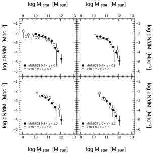
1.7 The evolution of the stellar mass function . . . 24

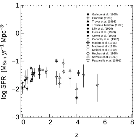
1.8 The cosmic star formation density . . . 26

1.9 Downsizing: Cowie et al. (1996) . . . . 27

2.1 MUNICS field geometry . . . 30

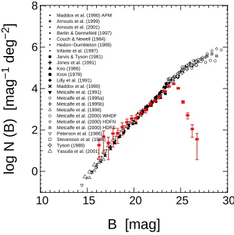
2.2 B-band galaxy number counts . . . 33

3.1 Object classification in J₋K vs. K diagram and based onχ2 . . . 37

4.1 Illumination function of MOSCA with Grism Green 500 . . . 44

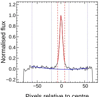
4.2 Definition of extraction and sky apertures . . . 45

4.3 Wavelength calibration lamp spectrum . . . 47

4.4 Test of quality of flux calibration . . . 48

4.5 Spectrum analysis and quality control plot . . . 49

4.6 Confidence class examples . . . 52

5.1 Redshift distribution . . . 56

5.2 Large-scale structure in S2F1 and S6F5 . . . 57

5.3 Histogram of redshift differences; comparison to SDSS EDR . . . 58

5.4 Colour and magnitude distributions, part 1 . . . 59

5.5 Colour and magnitude distributions, part 2 . . . 60

5.6 Redshift sampling rate . . . 61

5.7 Redshift success rate . . . 61

5.8 Sky coverage . . . 62

5.9 Comparison of photometric and spectroscopic object classification . . 64

5.10 V₋J colour histogram of stars . . . . 64

5.11 Composite stellar spectra . . . 65

6.1 k(z)corrections . . . 71

(12)

xii LIST OFFIGURES

6.3 J-band luminosity function from spectroscopic observations . . . 74

6.4 Kolmogorov–Smirnov test for M_K: MUNICS versus local samples . . 76

6.5 Kolmogorov–Smirnov test for M_J: MUNICS versus local samples . . 76

6.6 Kolmogorov–Smirnov test for M_Kand M_J for different redshifts . . . 77

6.7 Likelihood estimate for luminosity function evolution . . . 81

6.8 6dFGS-DR1: Redshift histogram and luminosity functions . . . 84

6.9 LF evolution based on 6dFGS . . . 85

6.10 Halo mass function and galaxy luminosity function . . . 87

6.11 Comparison of K-band luminosity function to semi-analytic models . 89 7.1 Completeness fractions for MUNICS_I and MUNICS_B . . . 94

7.2 Template galaxy SEDs, distribution of SED types . . . 96

7.3 Photometric redshift examples . . . 97

7.4 Photometric redshift histograms . . . 99

7.5 Comparison of photometric and spectroscopic redshifts . . . 100

7.6 Comparison of K, I and B-selected photometric redshifts . . . 101

7.7 M_Iand M_Bversus photometric redshift . . . 102

7.8 Comparison of photometric and spectroscopic object classification . . 104

8.1 Colour distribution of K, I and B-band selected galaxies . . . 107

8.2 Photometric redshift probability distributions . . . 108

8.3 Selection effects and the LF . . . 110

8.4 MUNICS_I: B-band LF . . . 111

8.5 MUNICS_I: B-band LF evolution . . . 112

8.6 MUNICS_I: I-band LF . . . 113

8.7 MUNICS_I: I-band LF evolution . . . 114

8.8 MUNICS_I: K-band LF . . . 115

8.9 MUNICS_I: K-band LF evolution . . . 116

8.10 MUNICS_I: Evolution of LF in B, I and K . . . 117

8.11 MUNICS_I: Galaxy luminosity density . . . 119

8.12 Star formation rate density from MUNICS & FDF . . . 121

8.13 Downsizing: SFR versus M_K . . . 123

8.14 Downsizing: [OII] equivalent width versus M_K . . . 124

8.15 Downsizing: Specific SFR versus stellar mass (MUNICS_I) . . . 125

8.16 Downsizing: Specific SFR versus stellar mass (MUNICS_B) . . . 126

8.17 Downsizing: Specific SFR versus stellar mass (MUNICS_K) . . . 127

8.18 Downsizing: Specific SFR versus stellar mass for different ages . . . 128

8.19 Evolution of SSFR with redshift . . . 129

A.1 Completeness of spectroscopy in MUNICS . . . 160

B.1 MUNICS_K & MUNICS_I: Comparison of photometry . . . 161

B.2 MUNICS_I & MUNICS_B: Comparison of photometry . . . 163

(13)

List of Tables

1.1 Cosmological parameters from WMAP . . . 3

1.2 Important cosmic epochs . . . 8

1.3 Galaxies at z>5 . . . 22

2.1 Completeness limits for MUNICS . . . 31

2.2 MUNICS fields . . . 31

2.3 MUNICS B-band observations and calibration . . . . 32

3.1 Results of test of image-based object classification . . . 36

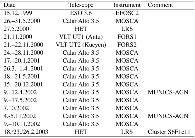
3.2 Observing runs . . . 38

3.3 Technical characteristics of spectrographs . . . 39

3.4 Typical exposure times of spectroscopic observations . . . 39

4.1 Description of confidence classes . . . 50

4.2 Small part of spectroscopic catalogue . . . 51

5.1 Spectroscopy of MUNICS fields . . . 54

5.2 Distribution of confidence classes . . . 55

6.1 K-band luminosity function data . . . . 77

6.2 J-band luminosity function data . . . 78

6.3 Kolmogorov–Smirnov test for M_K: MUNICS versus local samples . . 78

6.4 Kolmogorov–Smirnov test for M_J: MUNICS versus local samples . . 79

6.5 Summary: Measurements of the K-band luminosity function . . . . . 82

6.6 Summary: Measurements of the J-band luminosity function . . . 83

6.7 Summary: Measurements of the H-band luminosity function . . . . . 83

7.1 Number of detected objects . . . 93

7.2 Parameters of analytic approximation to redshift histograms . . . 101

8.1 MUNICS_I: Schechter parameters . . . 117

8.2 MUNICS_I: LF evolution . . . 118

8.3 Slope of SFRD at low redshift: Previous results . . . 120

(14)

(15)

List of Abbreviations & Acronyms

To help readers from a non-astronomical background to find their way in the jungle of astronomical abbreviations and acronyms, the meaning of (hopefully) all of those which can be found in this work is given below. Common abbreviations for astronom-ical journals which are used in the bibliography of this thesis are set in italics.

2dFGRS 2-degree Field Galaxy Redshift Survey

2MASS 2-Micron All-Sky Survey

A&A Astronomy and Astrophysics

ACS Advanced Camera for Surveys

AGN Active Galactic Nucleus, Nuclei

AJ The Astronomical Journal

ApJ The Astrophysical Journal

ApJS The Astrophysical Journal Supplement Series

ARA&A Annual Reviews of Astronomy and Astrophysics

Boojums Blue Objects Observed Just Undergoing Moderate

Starburst

CAFOS Calar Alto Faint Object Spectrograph

CCD Charge-Coupled Device

CDFS Chandra Deep Field South

CfA Harvard-Smithsonian Center for Astrophysics

CFRS Canada–France Redshift Survey

CMB Cosmic Microwave Background

COBE Cosmic Background Explorer

DRG, DRGs Distant Red Galaxy, Galaxies

EFOSC ESO Faint Object Spectrograph

ERO, EROs Extremely Red Object, Objects

ESO European Southern Observatory

FDF FORS Deep Field

FP Fundamental Plane (of elliptical galaxies)

FORS FOcal Reducer and Spectrograph

(16)

xvi LIST OFABBREVIATIONS& ACRONYMS

GOODS Great Observatories Origins Deep Survey

HDF Hubble Deep Field

HET Hobby-Eberly Telescope

HST Hubble Space Telescope

IMF Initial Mass Function

IRAF Image Reduction and Analysis Facility

IRAM Institut de Radio Astronomie Millimétrique

IRAS InfraRed Astronomical Satellite

JCMT James Clerk Maxwell Telescope

LAE, LAEs Lyman-Alpha Emitter, Emitters

LBG, LBGs Lyman-Break Galaxy, Galaxies

LF, LFs Luminosity Function, Functions

LRS Low-Resolution Spectrograph

MNRAS Monthly Notices of the Royal Astronomical Society

MOS Multi-Object Spectroscopy

MOSCA Multi-Object Spectrograph for Calar Alto

MUNICS MUnich Near-Infrared Cluster Survey

NICMOS Near-Infrared Camera and Multi-Object Spectrometer

PASJ Publications of the Astronomical Society of Japan

PASP Publications of the Astronomical Society of the Pacific

Phys. Rev. Physical Review

PSF Point-Spread Function

RMS Root Mean Square

SAM, SAMs Semi-Analytic Model, Models

SCUBA Sub-mm Common-User Bolometer Array

SDSS Sloan Digital Sky Survey

SED Spectral Energy Distribution

SFH Star Formation History

SFR Star Formation Rate

SFRD Star Formation Rate Density

SPIE Society of Photo-optical Instrumentation Engineers

SSFR Specific Star-Formation Rate

UDF (Hubble) Ultra Deep Field

ULIRG, ULIRGs Ultra-Luminous InfraRed Galaxy, Galaxies

UV Ultra-Violet

VLT Very Large Telescope

WFPC 1, 2 Wide-Field Planetary Camera 1, 2

(17)

Chapter 1

Introduction: Studying Galaxy

Evolution with Redshift Surveys

In this thesis results for the evolution of galaxies derived from a near-infrared selected galaxy redshift survey are presented. This chapter will provide an introduction to cosmology and galaxy formation (Section 1.1; see, e.g., Peebles 1980, Carroll et al. 1992, Peebles 1993, Peacock 1999, Coles & Lucchin 1995, Longair 1998), followed by a brief outline of results concerning the selection of galaxies at different cosmic epochs and their characteristics (Section 1.2), and a summary of statistical properties of galaxy populations used to trace their evolution (Section 1.3). Readers who are only interested in a summary of techniques and results in the field of galaxy evolution are kindly asked to skip Section 1.1 However, I do believe it to be important to place research results in a broader context.

1.1 Setting the Stage: The Formation of Galaxies within the

Framework of Cosmology

1.1.1 The Cosmological Standard Model

The evolution of the universe on large scales is governed by gravity which, on the other hand, is described by the field equations of Einstein’s General Theory of Relativity (Einstein 1916, Weinberg 1972)

R_{i j} ₋ 1

2Gi jR −ΛGi j = 8πG

c4 Ti j. (1.1)

Here R

i j and R are the Ricci tensor and scalar, respectively (describing space

(18)

2 CHAPTER1. STUDYING GALAXYEVOLUTION WITH REDSHIFT SURVEYS

The cosmological principle states that the universe is homogeneous and isotropic on large scales. This assumption was not invented to make physicists’ lives easier, of course, but can to some extent be verified for large cosmic scales. In this case the metric of the universe fortunately takes a simple form known as the Robertson-Walker

metric (Robertson 1935, 1936a, b, Walker 1935):

ds2 = c2dt2₋R2(t)

dr2

1₋kr2 +r

2 _d_θ2 ₊_sin2_θ_d_φ2

(1.2)

Here(r,θ,φ,t) are the space-time coordinates, R(t) is an unknown function de-scribing the dynamic evolution of the universe, and k can – by choice of units for

r – be fixed to +1, 0 or ₋1 for positively curved, flat and negatively curved space,

respectively (Weinberg 1972).

Using this form of space-time metric, relatively simple formulae can be derived for the dynamic behaviour of the universe (Friedmann 1922). These Friedmann equations read

˙

R2 = 8πG

3 ρR

2₊ 1

3c

2_Λ_R2

−k c2

(1.3)

¨

R = ₋4πG

3 R

ρ +3 p

c2

+ 1

3c

2_Λ_R

In these equations, ρ denotes the total energy density of the universe, p is the pressure, Λis the cosmological constant, and k is the curvature of space, i.e. k= +1 for a closed, k=₋1 for an open, and k=0 for a flat universe (Weinberg 1972). This geometrical curvature of space is governed by the density of the universe. Together with a knowledge of the equation of state p(ρ)the Friedmann equations can be solved for R(t). Furthermore we define the critical densityρcas

ρc ≡ 3H 2

8πG (1.4)

where the famous Hubble parameter H, the current value of which, usually just called the Hubble constant

H₀ _≡ H(t₀) _≡ h 100 km s−1Mpc−1, (1.5)

impertinently tried to escape from precise determination for decades, is given by the rate of expansion of the universe,

H = R˙

R. (1.6)

The we can re-write the first of the two Friedmann equations in the following form:

kc2

(19)

1.1. THEFORMATION OFGALAXIES IN THE UNIVERSE 3

Table 1.1: Cosmological parameters from WMAP and combination of WMAP with other data (Spergel et al. 2003), except forΩ_r,₀.

Quantity Value Comment

Ω_r_,₀ _∼10−4 radiation, relativistic particles (Peacock 1999)

Ω_b,₀ 0.047_±0.006 baryonic matter

Ω_m,₀ 0.29_±0.07 baryonic and dark matter

Ω_Λ_,₀ 0.73_±0.07 dark energy, computed fromΩ_tot_,₀₋Ω_m,₀

Ω_tot_,₀ 1.02_±0.02 total density budget

h 0.72_±0.05 Hubble constant

where we have defined the density parameters Ωfor the matter component (Ωr), for the radiation and relativistic particles (Ωr) and for the cosmological constant Λ (Ω_Λ), respectively, by setting

Ω _≡ ρ

ρc. (1.8)

Quite obviously, the curvature of the universe (as represented by the constant k) is directly connected to the density parameter(s) of the universe: If they add up to one, then space is flat (k=0). It also shows that the knowledge of the density parameters of the universe’s constituents and the knowledge of the Hubble constant suffice to describe the evolution of the scale factor.

Note that the density parameters are time-dependent quantities and scale differ-ently with redshift: Ω_Λ(z) =Ω_Λ_,₀, Ωm(z) =Ω_m,₀(1+z)3 _and _Ωr₍_z_{) =}_Ω

r,0(1+z)4. According to measurements of the cosmic microwave background (combined with other cosmological experiments), the contributions of the main constituents of the uni-verse can be found in Table 1.1.

One family of world models described by the Friedmann equations are models for an expanding universe. After Hubble’s discovery of the redshift-distance relation (Hubble 1929), which was soon interpreted as evidence for a cosmological expansion, the Big Bang model for the history of the universe emerged. In this scenario, the universe expands from a hot initial state. The precise history of this expansion is governed by the energy content of the cosmos.

1.1.2 The Cosmological Redshift

In the first half of the 20th century, it was discovered that the spectral lines of galaxies are, in general, shifted towards longer wavelength.1 To quantify this shift, we define the redshift z of a galaxy as

1_{Local gravitational attraction results in peculiar velocities superimposed on the general flow. Hence}

(20)

z _≡ λobs−λemit

λemit

, (1.9)

whereλ_obs is the observed wavelength of a spectral line, whileλ_emit is the wave-length as emitted by the galaxy.

This redshift of galaxies is interpreted as a result of the universe’s expansion. As swhon above, Assuming that the universe is homogeneous and isotropic, the expansion is described by the variation of the scale factor R(t), and it can be easily shown that

1+z = R(tobs)

R(t_emit), (1.10)

where the evolution of the scale factor R(t)is governed by the Friedmann equa-tions (1.3).

1.1.3 The Early Phases in the Life of the Universe

The Planck Epoch

We will briefly summarise the early stages in the universe’s life. The cosmos starts out in an era where it was governed by the weird (and unknown) laws of quantum gravity. This period, known as the Planck epoch, is characterised by the Planck time

t_P_'10−43s.2Classical gravity is invalid during this epoch, and since we lack a theory of quantum gravity any physical phenomena at these times belong to the realm of speculation.

Inflation

Cosmic inflation, a phase of exponential expansion of the universe at t_∼10−35s (Guth 1981, see Narlikar & Padmanabhan 1991 for a review), has been proposed to solve

2_{The Planck time t}

P(as well as the Planck length`Pand the Planck mass mP) is given by a ‘natural’

combination of the fundamental constants G (the gravitational constant), c (the speed of light in vacuum) and h (Planck’s constant):

t_P =

Gh c5

1/2

' 10−43s

`_P =

Gh c3

1/2

' 10−35m (1.11)

m_P =

hc G

1/2

' 10−7kg

(1.12)

(21)

several intriguing difficulties of the standard model, but may also serve as a source of the initial fluctuations needed for forming structures in an otherwise rather boring homogeneous universe (see Section 1.1.4).

One of the problems of the standard model is the ‘flatness problem’, or the ques-tion: Why is the curvature of the cosmos so close to zero? Inflation solves this natu-rally: A small region of space, exponentially expanded to very many times its orgininal size, will finally have a flat geometry – (almost) irrespective of its initial curvature.

In much the same way inflation also solves the ‘horizon problem’: Why does the cosmos look so similar everywhere, although its individual parts cannot all have been causally connected given the finite speed of light? Again, a phase of exponential ex-pansion, where the universe observed today originates from a small, causally con-nected region of space could solve this problem.

The Thermal History of the Universe

The early history of our cosmos is largely governed by its temperature. To under-stand this thermal history it is essential to know the way temperature evolves with cosmic time. A hot initial state with steadily decreasing temperature is one of the key ingredients of the hot big bang model which so successfully explains things like cos-mic nucleosynthesis and the coscos-mic cos-microwave background radiation discussed below. The temperature of the radiation filling the universe is related to the expansion. As-suming that we measure a temperature T₀for the background radiation field today, the temperature Trof the radiative component scales with the redshift z in the following

way:

Tr = T0(1+z) (1.13)

This can be derived from the energy densityεr of black body radiation which is

εr∝T4. On the other hand, this energy density is proportional to the number density n of photons times their energy hν. From the fact that n∝(1+z)3 _andν ∝₍₁₊_z₎_(the cosmic redshift), equation (1.13) follows immediately.

Big Bang Nucleosynthesis

During the first few minutes after the Big Bang, the light elements deuterium (D or2₁H), helium (3₂He and4₂He) and lithium (7₃Li) were formed in a process named primordial nucleosynthesis (Boesgaard & Steigman 1985, Tytler et al. 2000). Heavier elements cannot be produced because of the lack of stable elements with atomic masses of 5 and 8, and because of the increasing importance of the Coulomb barrier, particularly in a cooling universe. Within the standard model, primordial nucleosynthesis is one of the key tests of the hot big bang scenario because it makes relatively precise predictions for the relative abundances of those light elements depending on only one cosmological parameter, the baryon-to-photon ratio η _≡n_b/n_γ (see Figure 1.1).3 The other two

3_{Baryons are all strongly interacting elementary particles with half-integral spin and relatively high}

(22)

Figure 1.1: Abundances of light elements as a function of the baryon-to-photon ratio

η (here expressed by the baryon density) as predicted by models of big bang nucle-osynthesis (for h=0.65; taken from Tytler et al. 2000). The rectangles represent the 95% confidence regions for measured abundances.

important parameters for primordial nucleosynthesis are the number of neutrinos and the decay time of the neutron.

The general trend withη in Figure 1.1 can be easily understood: The higher the baryon density, the earlier nucleosynthesis starts, and hence the more nucleons end up in heavier elements. The dip in the abundance of lithium is due to the fact that 7₃Li is produced via two channels, either 4₂He(3₁H,γ)7₃Li or4₂He(3₂He,γ)7₄Be and subsequent decay (Yang et al. 1984).

The successful prediction of the observed abundance ratios of the light elements is a strong piece of evidence in favour of the hot big bang model.

Matter-Radiation Equality

In the beginning the universe was dominated by radiation, i.e. the energy density of radiationεrgreatly exceeded the one contained in matterεm:εrεm. However, since with cosmic time the radiative energy density drops off asεr∝T4∝(1+z)4_(see equa-tion (1.13)) while the matter energy density decreases withεm∝ρ ∝(1+z)3_{, there is} a time whenεr=εm: Matter and radiation contribute equal amounts to the cosmic en-ergy budget. At this epoch (at zeq'3300) of matter-radiation equivalence the universe

(23)

evolves from a radiation-dominated world to the matter-dominated universe we know today. Moreover, this is the time when density fluctuations in the matter component can begin to grow to form the structures observed today.

Recombination, Decoupling the the Surface of Last Scattering

At early times matter and radiation were tightly coupled by the process of Thomson scattering. However, as the universe expands, there is a dramatic shift in the rate between the typical collision time-scale and the time-scale for the cosmic expansion: While the collision time-scaleτc grows asτc∝ρ_m−1∝(1+z)3_{, the cosmic expansion} evolves more slowly as τ_H ∝(1+z)−3/2 _{(for a matter-dominated universe). Hence} there exists a transition period in cosmic history when scattering takes place on time-scales growing larger than the rate of cosmic expansion. This marked change in the history of the universe is known as the decoupling of radiation and matter.

At some point the coupling of matter and radiation certainly had to end: When the temperature fell to T<

∼104K, the electrons and the ions combined for the first time in

cosmic history, an event which is somewhat unfortunately known as the epoch of

re-combination. At that time, the intimate liaison between matter and radiation, mediated

by the process of Thomson scattering of photons with free electrons, finally comes to a doleful end. However, this is not an instantaneous process: Ionisation degrees X of

X=0.9 is reached at z_∼1500, X=0.5 at z_∼1400, and at z_∼1300 the ionisation is still 10% (X=0.1).

All this is closely related to the background radiation field which we will discuss below. The background photons were free to travel after decoupling, and the time when their optical depthτ was equal to one (τ =1) is known as the time of last scattering. These three time-scales are closely related but follow from different definitions. To clarify matters, I have summarised these epochs in Table 1.2.

The Cosmic Microwave Background

The cosmic microwave background is the relic radiation from the hot big bang. It was discovered by chance (Penzias & Wilson 1965, Dicke et al. 1965), although there had been theoretical considerations predicting this kind of radiation before.

The cosmic background radiation we observe today has a almost perfect blackbody spectrum4corresponding to a temperature of T=2.726_±0.002 K (Fixsen et al. 1996). However, small temperature fluctuations of the order∆T/T_∼10−5are observed in the CMB. These can be interpreted as signatures of density perturbations in the epoch of recombination and will be discussed in more detail in Section 1.1.4.

4_{According to Planck’s law, the radiation intensity B}

ν(T)emitted by a black body at temperature T and frequencyνis given by

B_ν(T) = 2h

c2 ν3

exp

hν kT

−1

, (1.14)

(24)

8

C

H

A

P

T

E

R

1

.

S

T

U

DY

IN

G

A

L

A

X

Y

E

V

O

L

U

T

IO

N

W

IT

H

R

E

D

S

H

IF

T

S

U

R

V

E

Y

S

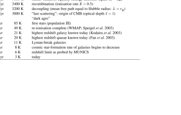
Table 1.2: Summary of important epochs in the history of our universe showing their redshift, time, (radiation) temperature and definition.

zeq, zrec and z_dec are calculated using the formulae given in Kolb & Turner (1990) with the cosmological parameters presented in Spergel

et al. (2003).

Redshift Time Temperature Event

10−43s 1032K Planck epoch: realm of quantum gravity

10−35_s ₁₀27_K _{epoch of inflation (?): exponential expansion, first seeds of structure}

10−7s 1014K formation of nucleons (protons and neutrons)

15 min 108K end of primordial nucleosynthesis

zeq'3300 0.06 Myr 9000 K matter-radiation equality (energy densities equal: εr=εm)

zrec'1260 0.43 Myr 3400 K recombination (ionisation rate X=0.5)

z_dec_'1160 0.49 Myr 3200 K decoupling (mean free path equal to Hubble radius:λ =r_H)

z_ls_'1100 0.53 Myr 3000 K “last scattering”: origin of CMB (optical depthτ=1)

“dark ages”

z_'30 0.1 Gyr 85 K first stars (population III)

z_'17_±5 0.2 Gyr 49 K re-ionisation complete (WMAP; Spergel et al. 2003)

z=6.6 0.8 Gyr 21 K highest redshift galaxy known today (Kodaira et al. 2003)

z=6.4 0.9 Gyr 20 K highest redshift quasar known today (Fan et al. 2003)

z_∼3 2.2 Gyr 11 K Lyman-break galaxies

z_∼2 3.2 Gyr 8 K cosmic star-formation rate of galaxies begins to decrease

z_∼1 5.8 Gyr 6 K redshift limit as probed by MUNICS

(25)

Figure 1.2: Temperature fluctuations in the cosmic microwave background as mea-sured by WMAP (Spergel et al. 2003).

1.1.4 Formation of Structure in the Universe

The General Picture

The homogeneity of the universe on large scales is well established. It is also evident from the cosmic microwave background (CMB) the temperature of which is highly homogeneous with fluctuations∆T/T _∼10−5. Today, however, we observe prominent structure in the form of galaxies, clusters and super clusters. For example, the density in a galaxy is about 105 _{times the average density of the universe, and clusters of} galaxies reach over-densities of 102. . . 103. So how did this structure form?

It is thought to have developed from small initial fluctuations in the universe’s density. The foot prints of these fluctuations can still be observed in the temperature variations in the CMB (see Figure 1.2). The microwave background mirrors the fluc-tuations at z_∼1100, when, at the end of the epoch of recombination of electrons and ions, the universe became transparent to electromagnetic radiation (“surface of last scattering”).

These fluctuations then grew under the influence of the gravitational interaction mainly caused by the dark matter present in the universe. At a later time the baryonic gas streamed into these dark matter haloes, formed stars and thus created the luminous matter observed in galaxies.

The first stars, the so-called “population III stars”5, formed at redshifts z_∼20. . .30 in mini dark-matter haloes ofM_∼₁₀6_M

. Due to the lack of heavy elements present

in today’s stellar objects they had vastly different properties: Their typical masses were close to∼100 M, and they ended their brief life enriching the universe with the first 5_{The name ‘population III’ tries to extend the concept of stellar populations introduced by Baade}

(26)

heavy elements (Bromm & Larson 2004).

In a universe dominated by cold dark matter – which is the favoured model these days – galaxies grow hierarchically: The first structures to form are low-mass objects which then grow by subsequent merging to the massive galaxies observed today.

However, while the gravitational dynamics of cold dark matter can be easily mod-elled and very successfully explains the large-scale properties of the cosmic matter distribution, the situation on galaxy-size scales is less clear. The reason is the “dirty physics” of gas cooling, star formation, and stellar feedback on the surrounding gas which escapes detailed calculations by means of its complexity.

Linear Theory of Density Perturbations

Imagine small perturbations in the matter densityρand the velocity field u which can be parameterised asρ(x,t) =ρ¯(t)(1+δ(x,t))and u=_Rx˙₊_{v, where x are comoving} coordinates, and the density contrastδ and the peculiar velocity v represent small per-turbations. Inserting this into the basic equations of fluid dynamics, the equation of continuity, Euler’s equation and Poisson’s equation, neglecting higher order perturba-tions, and introduing Fourier transformed quantities δ(x,t) =∑_kδ_k(t)exp(ik_·x), we obtain the linear perturbation equation for a matter-dominated universe

d2δ_k

dt2 +2

˙

R R

dδ_k

dt − 4πG ¯ρ−

csk

R

2!

δ_k = 0, (1.15)

where cs is the sound speed. Equation (1.15) is a wave equation with decaying

and non-decaying solutions. So how much do perturbations grow in our universe? We have already shown that at z∼1100 we observe temperature fluctuations in the CMB corresponding to density fluctuations in the baryonic component of δ_b _'5_· 10−5. How much would these fluctuations grow until today? For a universe with the density parametersΩ_m,₀'0.3 andΩ_Λ'0.7 (similar to the ones given in Table 1.1), the growth of structure is about 80% of the growth observed in a Einstein-de Sitter universe with Ω_m,₀=1, Ω_Λ =0 universe (Carroll et al. 1992). For the Einstein-de Sitter universe, the scale factor R grows as R∝t2/3, and the non-decaying solution of the linear perturbation equation asδ_k∝t2/3∝R∝(1+z). Thus, baryonic fluctuations of the amplitude observed in the CMB could grow toδ_b<0.05 today, much less than the density contrast observed in galaxies and clusters today. Hence “dark matter” is needed to explain the structures in our universe today!

Density Fluctuations and the Cosmic Microwave Background

One very important finding about the CMB is the existence of temperature fluctuations of the order∆T/T _'10−5(see Figure 1.2). These are interpreted as imprints of still small density fluctuations in the early universe which are the seeds of the structure observed in the local universe: For adiabatic perturbations, fluctuations in temperature

(27)

Figure 1.3: The angular power spectrum (more precisely l(l+1)C_l/2π with C_ldefined in equation (1.18)) of temperature fluctuations in the cosmic microwave background as measured by the WMAP satellite (points, Hinshaw et al. 2003) as well as the best-fitting model (line, Spergel et al. 2003).

∆ρ_b ρ_b = 3

∆T

T . (1.16)

Note that the power spectrum of these temperature fluctuations in the CMB are an efficient way to derive cosmological parameters (see e.g. Hu & Dodelson 2002, Scott & Smoot 2004).

To get the angular power spectrum, the temperature variations on the sky are ex-pressed through a sum over spherical harmonics:

∆T(θ,φ)

T =

∞

∑

l=0

+l

∑

m=−l

a_lmY_lm(θ,φ) (1.17)

The angular power spectrum C_l is then computed from the coefficients a_lmby

C_l _{≡ h}a_lm2i = 1

2l+1

+l

∑

m=−l

a_lma∗_lm (1.18)

The most accurate measurement of this angular power spectrum so far was done with the WMAP satellite and is shown in Figure 1.3 (Hinshaw et al. 2003).

The general shape of this curve can be understood in terms of three distinct effects. On large angular scales (l<

∼100) the dominant contribution is from the Sachs-Wolfe

(28)

0 2 4 6 8 10

0 2 4 6 8 10 12 14

z

Lookback time [Gyr]

Figure 1.4: The cosmological look-back time versus redshift. A cosmology withΩm= 0.3,Ω_Λ=0.7 and H₀=70 km s−1Mpc−1was assumed.

gravitational potential∆Φleading to (I) gravitational redshift and (II) time dilation for photons climbing out of the potential well:

∆T

T =

_∆Φ

c2

| {z } I

+

−2 3

∆Φ

c2

| {z }

II

= 1

3

∆Φ

c2 (1.19)

The Sachs-Wolfe effect is responsible for the low-l plateau in the angular power spectrum shown in Figure 1.3.

At intermediate scales (100_∼l<

∼1000) we can see prominent peaks in the angular

power spectrum (see Figure 1.3). These are caused by gravity-driven acoustic oscil-lations before recombination and are thus called the acoustic peaks. The position of the peaks is connected to the sound horizon at the time of last scattering and therefore probes the curvature of the universe (i.e.Ω), while its height is governed by the baryon contentΩ_bof the universe.

On the smallest scales (1000<

∼l) the oscillations are damped by two effects. The

(29)

1.2. OBSERVINGGALAXIES ATLOW ANDHIGHREDSHIFT 13

1.1.5 Looking Back: Redshift and Galaxy Evolution

We live in an evolving universe. But how can we study the evolution of galaxies with cosmic time? Since the life times of human beings are much shorter than the age of the universe, we obviously cannot do this for individual galaxies. But due to the finite speed of light we can study galaxies at different epochs in the cosmologi-cal history: The higher the redshift at which we observe galaxies, the longer it took their light to travel to our telescopes, and thus the younger are the galaxies we see at this redshift. This is expressed by the cosmic look-back time, which is shown in Figure 1.4 for a “standard” cosmological model with Ωm =0.3, Ω_Λ =0.7 and

H₀=70 km s−1Mpc−1, close to the values determined by the Wilkinson Microwave Anisotropy Probe (WMAP; Spergel et al. 2003, see Table 1.1). With the MUNICS redshift survey described in this thesis, we can investigate the evolution of galaxy pop-ulations since z_∼1, when the universe had only half of its present age.

1.2 The Evolution of Galaxies with Cosmic Time: Observing

Galaxies From Low to High Redshift

In the last decades we have learned a lot about the evolution of galaxies in the uni-verse. Much of this progress is due to improved observational techniques allowing us to study both larger samples of local galaxies and deeper samples probing galaxies out to redshifts z_∼5 or beyond.

In principle we can distinguish several different methods to obtains samples of galaxies. Firstly, there are wide-field surveys which, being usually not very deep, pro-vide large numbers of galaxies at lower redshifts. Secondly, one can invest observing time on deep exposures of smaller fields, so-called ‘pencil-beam surveys’, which trace galaxies out to high redshift. Thirdly, one can use broad-band photometric information to select galaxies at different redshifts. Extremely Red Objects (EROs) and Lyman-Break Galaxies (LBGs), amongst others, fall into this category.

It is important to note that with different selection techniques one builds up samples of galaxies from different populations and at different redshifts. The challenge remains to construct a unifying picture of galaxy formation and evolution from these different samples.

In the following, I will summarise important observational results on galaxy sam-ples drawn from different selection schemes.

1.2.1 Surveys of the Local Universe

(30)

J, H and Kswith a limiting K-band magnitude of Ks'13.5. In parallel, large

spectro-scopic surveys like the 2-degree Field Galaxy Redshift Survey (2dFGRS, Folkes et al. 1999) provide catalogues of thousands of redshifts for galaxies, mapping a consider-able portion of the local universe. The 2dFGRS contains more than 220 000 galaxies with b_J≤19.45 in 1500 square degrees selected from photographic plates of the APM survey (Maddox et al. 1990a).

1.2.2 The Universe at Midlife

By the 1980s, the increased number of 4-m class telescopes and advances in electronic detector technology enabled deeper surveys of the universe out to redshifts z _∼ 1, when the universe had about half of its present age (see Colless 1997, Ellis 1997 for reviews).

Many traditional surveys were conducted in the B band using photographic plates at Schmidt telescopes (Schmidt 1931, Wilson 2004). When multi-object spectrographs became available at 4-m class telescopes, many groups started follow-up observations of these surveys. One noteworthy redshift survey of that kind is the Autofib Redshift Survey probing the evolution of the luminosity function out to redshifts z ∼ 0.8 with roughly 1700 galaxy redshifts (Ellis et al. 1996, Heyl et al. 1997).

In the middle of the 1990s, the I-band selected Canada–France Redshift Survey (CFRS) marked an important point in the study of galaxy evolution with redshift sur-veys. The selection in the I band made it possible to study the evolution of the evolved, massive galaxies rather than star forming galaxies picked up in the more traditional

B-band selected samples. The CFRS comprises spectra of more than 1000 objects

with 17.5_≤I_AB_≤22.5, 591 of which are galaxies with secure redshifts in the range 0_≤z_≤1.3. A series of papers presented not only the technical details of the survey (Lilly et al. 1995a, b, Le Fèvre et al. 1995, Hammer et al. 1995), but more impor-tantly studies of the evolution of the luminosity function (Lilly et al. 1995c) and of the luminosity density and star formation rate density of the universe (Lilly et al. 1996), finding very little evolution in the luminosity and number density of red galaxies in the redshift range 0<z<1.

Selection in near-infrared filters like the K-band come even closer to a selection in stellar mass. When suitable near-infrared detectors became available at large tele-scopes, a number of K-band selected surveys were undertaken which can probe the evolution of massive galaxies out to redshift z _∼ 1. Examples for such surveys are the Hawaii Deep Fields (Cowie et al. 1994), the K20 Survey (Cimatti et al. 2002b) and the Munich Near-Infrared Cluster Survey (MUNICS; Drory et al. 2001b) on which this work is based.

1.2.3 Pencil-Beam Surveys

(31)

Moreover, they are affected by the variation of the galaxy distributions over the sky, an effect which is called ‘cosmic variance’.

Ground-based deep fields include the NTT Deep Field (NDF, Arnouts et al. 1999), the William Herschel Deep Field (WHDF, Metcalfe et al. 2001) and the FORS Deep Field (FDF, Heidt et al. 2003).

The most notable examples for these are, of course, the Hubble Deep Fields (HDFs, Ferguson et al. 2000), the HDF North (Williams et al. 1996) and the HDF South (Williams et al. 2000, Casertano et al. 2000), taken with the fantastic spatial resolution of the Hubble Space Telescope (HST). More recently, the Hubble Ultra Deep Field (UDF), a larger deep field taken with the new Advanced Camera for Sur-veys (ACS) on board HST was released. Because of the high resolution, studies of galaxy morphologies and sizes as well as their evolution with redshift are of special interest.

Many studies of galaxy morphologies have been carried out in the HDFs (e.g. Abraham et al. 1996, Odewahn et al. 1996, van den Bergh et al. 1996, Marleau & Simard 1998, van den Bergh et al. 2000, Kajisawa & Yamada 2001, Conselice et al. 2004). One general trend is the increasing number of galaxies with irregular appear-ance with redshift. Part of this trend may be attributed to the fact that the observed optical regime samples the galaxies ultraviolet light. In the ultraviolet, the light is dominated by the very young hot stars located in star forming regions displaying a patchy character also in the local universe. But this cannot explain all of the evolu-tion, especially it does not account for the increasing number of interacting systems observed in the HDFs (e.g. van den Bergh et al. 1996). Furthermore, Dickinson et al. (2003) find from an near-infrared selected sample of HDF-N galaxies that 50–75% of the present-day stellar mass density was in place by z_'1, but only 3–14% at z_'2.7. All this might suggest that the classical Hubble sequence of galaxy types (Hubble 1926) appeared at 1<

∼z<∼2.

Another important aspect which can be investigated with HDFs is the evolution of galaxy sizes. From the beginning it was obvious that the high redshift galaxies seen in the HDFs are very small, compact objects (Lowenthal et al. 1997, Bouwens

et al. 2003). Analysis of recent observations taken with HST’s Advanced Camera for

Surveys (ACS) in the course of the GOODS project (Great Observatories Origins Deep Survey, Giavalisco et al. 2004) confirm this evolutionary trend (Ferguson et al. 2004).

1.2.4 Extremely Red Objects

In the late 1980s and early 90s, with the advent of near-infrared imagers at large tele-scopes, a class of objects with very red near-infrared to optical colours was discovered, the so-called Extremely Red Objects (EROs, Elston et al. 1988, 1989, Hu & Ridgway 1994, Soifer et al. 1994, see also McCarthy 2004 for a complete review)6. The defining criterion is usually expressed in terms of R₋K colour, and typical definitions for EROs

are in the range R−K > 5. . .6. From the beginning they were thought to be either luminous star-forming galaxies at very high redshifts or evolved early-type galaxies at

6_{Sometimes these objects are also called ‘Extremely Red Galaxies (ERGs)’ However, in this work we}

(32)

redshifts z>

∼1. EROs have a surface density at the sky of∼0.4 arcmin−2 (Thompson

et al. 1999, Yan et al. 2000).

Since by the end of that decade there was more and more interest in near-infrared surveys of field galaxies, a wealth of papers on the photometric, morphological and clustering properties of EROs appeared in the literature.

The first detailed studies of one ERO called HR10 found by Hu & Ridgway (1994) revealed it to be a dusty starburst galaxy at redshift z=1.44 (Graham & Dey 1996, Cimatti et al. 1998, Dey et al. 1999).

Later studies of the spectral energy distributions (SEDs) or spectroscopic observa-tions of EROs confirmed that they are not a homogeneous class. While some authors found them to be early-type galaxies at z>

∼1 (e.g., Elston1989, Hu & Ridgway 1994),

others found indication for star-formation or AGN activity (e.g., Graham & Dey 1996). Most authors studying larger samples of EROs find a mix of both types. Cimatti

et al. (1999) find that 2 out of 9 EROs they studied seem to be dusty star-bursts,

while the rest are consistent with dustless evolved spheroidals at z>

∼0.8. Similar

re-sults for bright EROs are found by Saracco et al. (2003) who identify massive evolved galaxies at redshifts z>1. On larger samples most authors find both classes (Martini 2001, Cimatti et al. 2002a, Smail et al. 2002b, Väisänen & Johansson 2004, Yan et al. 2004c).

Different contributions from evolved early-type galaxies and dusty star-bursts to the ERO population found in these studies can likely be attributed to different mag-nitude limits, different colour selection criteria, and to field-to-field variations of the galaxy distribution (cosmic variance). Colour-colour diagrams may offer an easy way to distinguish these different populations (Pozzetti & Mannucci 2000).

Morphologically this dichotomy is confirmed. Some EROs show asymmetric mor-phologies (Graham & Dey 1996), others are well described by R1/4 profiles (de Vau-couleurs 1948) typical for elliptical galaxies (Treu et al. 1998, Elston et al. 1989). Yan & Thompson (2003) investigated the morphology of more than 100 EROs from HST imaging. They find that roughly one third of the sample consists of bulge-dominated galaxies, while the rest is comprised by disks. Furthermore, they find indications of merging activity for about 20 per cent of all EROs. As with the spectral properties, morphological studies of larger samples contain a mix of E/S0-like, spiral-like and irregular morphologies (Moriondo et al. 2000, Cimatti et al. 2003, Moustakas et al. 2004, Yan et al. 2004c), with different fractions caused by different selection tech-niques.

It is interesting to note that there is no strong correlation between spectral type and morphological classification (Moustakas et al. 2004, Yan et al. 2004c)

Studies of the angular ERO distribution indicate that they are strongly clustered with comoving correlation lengths of the order r₀ _' (10_±3)h−1Mpc, in the range of present-day elliptical galaxies (Yan et al. 2000, McCarthy et al. 2001, Roche et al. 2002) which have correlation lengths of r₀ _∼7 h−1Mpc, with the giant ellipticals hav-ing r₀ _∼ 11 h−1Mpc (see McCarthy 2004 and references therein).7 The clustering 7_{Clustering of galaxies in space can be described by the spatial two-point correlation function}_ξ₍_r₎

(33)

properties of the two contributing populations differ considerably in the sense that the old ellipticals show much more correlation. Daddi et al. (2002) measure a much smaller correlation length of r₀ =2.5 h−1Mpc for the star-forming EROs.

Radio and X-ray observations as well as optical spectroscopy reveal that only a small fraction of the ERO population is comprised of obscured AGN (Smail et al. 2002b, Cimatti et al. 2003, Yan et al. 2004c, Severgnini et al. 2004).

It has been suggested that EROs (or at least the evolved early-type galaxies con-tributing to the ERO population) might be an efficient tool to test current models of galaxy formation. Indeed, most present-day semi-analytic models seem to have dif-ficulties to match the observed number density of EROs at z>

∼1 (Cimatti et al. 1999,

Martini 2001, Daddi et al. 2002, Roche et al. 2002, Smith et al. 2002).

Recently, first observations with the Spitzer Space Telescope (formerly called SIRTF, the Space InfraRed Telescope Facility, Fanson et al. 1998) allowed the study of infrared properties of EROs and detected EROs at redshifts z∼2 and beyond (Yan

et al. 2004b, Wilson et al. 2004, Yan et al. 2004a).

1.2.5 Distant Red Galaxies

Recently, relatively red galaxies at redshifts z>

∼2 were discovered. Defined by there

red near-infrared colours, J₋K > 2.3, they are referred to as Distant Red Galaxies (DRGs, Franx et al. 2003, van Dokkum et al. 2003). DRGs apparently have stellar masses comparable to those of today’s early-type galaxies. Comparing DRGs and Lyman-Break Galaxies at redshifts z_∼3 (see next Section) at the same rest-frame optical luminosity, the DRGs seem to be dustier, more metal rich, more massive and older (van Dokkum et al. 2004).

1.2.6 Submillimeter Sources

Submillimeter (sub-mm) radiation of galaxies is mainly due to the emission from warm interstellar dust. The dust component absorbs the light of young, high-mass stars in star-forming galaxies and re-emits it at rest-frame wavelengths aroundλ_∼100µm (for typical dust temperatures of T'40 K). Quite naturally, the submillimeter emission is a measure of the galaxy’s current star-formation activity. The rest-frame peak of the dust emission implies that the k(z)corrections, which describe the change of flux in a given wavelength range due to the redshifting of the rest-frame spectrum, are negative, i.e. submillimeter sources are less affected by the effects of cosmological dimming (Blain & Longair 1993).

n(r)dV = n₀

h

1+ξ(r)idV (1.20) Thusξ(r)describes the excess number of galaxies at distance r from any given galaxy. On scales smaller than 10 h−1Mpc, the two-point correlation function can be well described by a power-law

ξ(r) = r0

r

γ

(1.21) with the comoving correlation length r₀. In the local universe measurements of galaxy clustering yield

(34)

When the Sub-mm Common-User Bolometer Array (SCUBA, Holland et al. 1999) became available at the 15-m James Clerk Maxwell Telescope (JCMT), astronomers were able to make sensitive images of the sky at sub-mm wavelengths, usually at

λ=850µm. They soon discovered a population of faint sub-mm sources in the distant universe (Smail et al. 1997). Many of these could be identified with Extremely Red Objects (EROs) in the near-infrared and optical regime (Smail et al. 1999), and are most likely massive, heavily star-forming and heavily obscured galaxies at redshifts

z>

∼2 (Smail et al. 2002a). In that respect, they are strikingly similar to the population of

Ultra-Luminous InfraRed Galaxies (ULIRGs) at low redshifts which were discovered in the 1980s by the InfraRed Astronomical Satellite (IRAS).

Difficulties with the interpretation of submillimeter galaxies remain. For one, SCUBA’s low angular resolution of only 15 arcsec makes optical identifications diffi-cult. (At millimetre wavelengths the 30-m IRAM telescope offers higher resolution.) Moreover, successful follow-up spectroscopy in the optical is hard to achieve since typical SCUBA sources are very red, dusty objects.

1.2.7 Exploring the ‘Redshift Desert’

We have already described the study of galaxies at redshifts z <

∼1.5 with traditional

redshift surveys and of Lyman-break galaxies (LBGs) at redshifts z>

∼2.5. The redshift

range in between, i.e. 1.5<

∼z<∼2.5 has traditionally been difficult to bridge due to the

lack of prominent spectral features at 4300Å <

∼λobs<∼9000Å characteristic for most spectrographs on this planet. Hence this regime had become known as the ‘redshift desert’.

This is somewhat unfortunate, because there are many pieces of evidence – e.g. the dramatically different appearance and properties of LBGs as compared to the local galaxy population – which might suggest that at these redshifts a significant change in galaxy properties might occur.

However, Adelberger et al. (2004) and Steidel et al. (2004) show how spectra of a large number of star-forming galaxies in this redshift range can be obtained by combining photometric colour pre-selection techniques with multi-object spectroscopy using a blue-optimised spectrograph at a 10-m class telescope. The principle of the photometric selection can be seen in Figure 1.5.

So far it is unclear how the population of this galaxies relates to the LBGs at z_∼3 and to galaxy samples at lower redshift, but the study of these objects will likely shed some more light on the process of galaxy evolution, especially in combination with galaxy samples at 1<

∼z<∼2 drawn from near-infrared selected surveys like the on-going

MUNICS-Deep project briefly described in Section 2.4.

1.2.8 Lyman-Break Galaxies

The best studied sample of high redshift galaxies are the Lyman-Break Galaxies (LBGs) at z _∼ 3 (see Giavalisco 2002 for a review). LBGs can be easily identified by optical photometry through filters designed to isolate the spectral discontinuity at

(35)

Figure 1.5: Illustration of the photometric selection technique for galaxies in the ‘red-shift desert’ (taken from Adelberger et al. 2004). Star-forming galaxies in a given redshift interval can be selected by choosing suitable combinations of galaxy colours.

is caused by a combination of the stellar spectral energy distributions, the intrinsic opacity of galaxies to Lyman continuum photons, and the influence of absorbers along the line of sight between the galaxy and the observer. The principle of this selection technique is illustrated in Figure 1.6.

Morphological investigations of LBGs making use of the high spatial resolution of HST show that they have very compact, bright cores (sometimes multiple) and are of-ten surrounded by a diffuse and asymmetric halo (Giavalisco et al. 1996, Steidel et al. 1996a). Star formation in these high-redshift galaxies thus occurs in very compact regions of high surface brightness. These findings might be interpreted to be evidence for a formation of the traditional Hubble sequence at lower redshifts than the LBG regime.

The spectra of LBGs resemble those of star-forming galaxies locally (Steidel et al. 1996b) and are remarkably uniform (Pettini et al. 2001). Detailed spectral analysis yields abundances of at least one tenth solar, making them rather metal rich for their epoch (Pettini et al. 2001). Moreover, the virial masses deduced from the measured ve-locity dispersions are of the order of 1010Mwithin a half-light radius of 2.5 kpc, with mass-to-light ratios of M/L_'0.15M/L corresponding to stellar populations be-tween 108and 109years old. Another very important finding is the existence of super-winds on galactic scales which certainly have a major effect on the star-formation histories of LBGs (Pettini et al. 2001).

(36)

Figure 1.6: Illustration of the photometric selection technique for LBGs (taken from Steidel et al. 1999a). The spectrum shown is a model spectrum of galaxy at redshift

z=3.15. Superimposed are the transmission curves of the three filters used in the pioneering studies by Steidel & Hamilton (1992). Clearly, one can efficiently pre-select samples of high-redshift galaxies using the Lyman continuum break in their spectra.

dustier, and younger galaxies are dustier and have higher star-formation rates. They try to explain these trends with a unified model in which a short burst of very rapid star formation of the order of hundreds solar masses per year is followed by a pe-riod of reduced star formation and dust extinction. The reduction of the extinction is probably governed by the huge outflows observed in LBGs, thereby causing the metal enrichment of the IGM (Adelberger et al. 2003).

Many studies of the clustering properties of LBGs have been performed (e.g., Adelberger et al. 1998, Giavalisco et al. 1998, Steidel et al. 1998, Giavalisco & Dick-inson 2001, Porciani & Giavalisco 2002). They find that LBGs are clustered with comoving correlation lengths of r₀ _' 4 h−1Mpc, with amplitudes comparable to the ones observed for present-day luminous spiral galaxies (the local galaxies cluster with correlation lengths of r₀ '5.7 h−1Mpc). This suggests that LBGs are associated with massive dark-matter haloes, and might be the progenitors of massive galaxies today.

1.2.9 Galaxies Beyond the LBG Regime

We conclude our overview of galaxies at different cosmic epochs by a summary of results on the highest redshift objects. To study galaxies beyond the realm of the Lyman-Break Galaxies (LBGs), i.e. galaxies at redshifts z>

∼4, one has several options.

(37)

1.3. STATISTICAL PROPERTIES OFGALAXIES 21

Ferguson et al. 2000, Williams et al. 2000, Casertano et al. 2000), the FORS Deep Field (FDF, Heidt et al. 2003) or the Ultra Deep Field (UDF) which probe the galaxy population out to z_∼5. . .6.

Other techniques are searches for the prominent Lyman-αemission line in narrow-band images in the optical, selection of radio-emitting objects, or photometric pre-selection (see Stern & Spinrad 1999, Taniguchi et al. 2003b for reviews). Since radio detection methods will yield samples of galaxies whose light is mostly dominated by the emission of their active nucleus, we will not discuss this technique in detail. Also, more modern photometric methods to find high-redshift AGN (e.g. Fan et al. 2001) will not be described here.

One popular technique is to search for the emission of the Lyman-α line of high-redshift galaxies. This was first suggested in a pioneering paper by Partridge & Peebles (1967) and led to the discovery of a number of galaxies at redshifts larger than five (see Table 1.3). Another method uses the spectral break aroundλ_'912Å and is thus similar to the pre-selection of LBGs at z_∼3. The only difference is that one uses

R-band or I-band drop-outs instead of U drop-outs as for the LBGs. This technique is

also very successful (see Table 1.3).

Note that although these two methods complement each other, they are in reality not completely independent. While the Lyman-break technique relies on the contin-uum shape only the appearance of an emission line at the location of the break helps in identifying the break. On the other hand, apart from the intrinsic asymmetry of the Lyman-α line, one popular criterion for the identification of a single Lyman-α line is the existence of continuum flux red-wards the line, and the total lack of it blue-wards. A variation of the drop-out approach is to use the objects’ photometry in several filters together with template spectral energy distributions (SEDs) to estimate their redshift. This ‘photometric redshift method’ has been pioneered by Baum (1962) and Koo (1985) and is widely used for obtaining redshifts today.

Kurk et al. (2004) used a different approach. The performed slitless spectroscopy in the wavelength region aroundλ _∼9100Å to search for Lyman-α emitters at z_∼6.5 and found one object at z=6.518.

The observed properties of these high-redshift galaxies are, of course, of particular interest. Although the number of confirmed objects at z>

∼5 is still very small, they allow

a glimpse at the very early stages of galaxy evolution. After all, at these redshifts, we see galaxies at an epoch when the universe was only 1 Gyr old.

Star-formation rates for these galaxies, as referred from their Lyman-α luminos-ity, are usually in the range 5. . .20 Myr−1, considerably lower than LBGs at z ∼3. Similar to other high-redshift objects, they show small physical sizes.

1.3 The Evolution of Galaxies with Cosmic Time: Statistical

Properties of Galaxies

1.3.1 The Galaxy Luminosity Function

(38)

Table 1.3: List of spectroscopically confirmed galaxies at redshifts beyond 5 (fol-lowing Stern & Spinrad 1999, Taniguchi et al. 2003b, Spinrad 2004, updated by the author).

z Technique Reference

6.58 narrow-band imaging Kodaira et al. (2003) 6.56 narrow-band imaging, lensed Hu et al. (2002)

6.55 serendipitous Stern et al. (2004)

6.54 narrow-band imaging Kodaira et al. (2003) 6.52 slitless spectroscopy Kurk et al. (2004)

6.33 Lyman-break Nagao et al. (2004)

6.17 narrow-band imaging Cuby et al. (2003)

5.87 Lyman-break Lehnert & Bremer (2003)

5.83 Lyman-break Dickinson et al. (2004)

5.78 Lyman-break Bunker et al. (2003)

5.77 serendipitous Dawson et al. (2001)

5.75 narrow-band imaging Rhoads et al. (2003)

5.74 narrow-band imaging, lensed Hu et al. (1999) 5.70 narrow-band imaging Rhoads et al. (2003) 5.69 narrow-band imaging Ajiki et al. (2002) 5.67 narrow-band imaging Rhoads et al. (2003) 5.66 narrow-band imaging Taniguchi et al. (2003a)

5.64 narrow-band imaging Hu et al. (1998)

5.60 Lyman-break Weymann et al. (1998)

5.58 serendipitous, lensed Ellis et al. (2001)

5.34 Lyman-break Spinrad et al. (1998)

5.34 Lyman-break Dey et al. (1998)

5.12 Lyman-break, lensed Frye et al. (2002)

Plotted in logarithmic units, it shows a characteristic shape with a linear behaviour at the faint end, and a sharp cut-off at high luminosity. This characteristic shape of the luminosity function is generally described by a Schechter function,

Ψ(L) = Φ∗

L∗

L L∗

α

exp

−_LL_∗

, (1.22)