Explicit object representation by sparse neural codes

(1)

Codes

Thesis by

Stephen Waydo

In Partial Fulfillment of the Requirements

for the Degree of

Doctor of Philosophy

California Institute of Technology

Pasadena, California

2008

(2)

c

2008 Stephen Waydo

(3)

Acknowledgments

Despite having only a single name on the cover, this thesis represents the work of a

great many people. Some have provided mentorship and guidance, some have directly

contributed to the work and the writing, and many more have helped me to become

who I am as a researcher and as a person. I have been exceedingly fortunate in the

friends and colleagues I have amassed over the years, and without them none of this

would have been possible.

Richard Murray has been my advisor since my first days at Caltech, and has been

an invaluable mentor as I have made the transition from coursework to independent

research. Richard is a continual fountain of enthusiasm no matter the subject area,

and has encouraged all of my explorations into a wide variety of subject areas as I

sought a suitable area for thesis research. Always available to help me make progress,

not with an answer but by finding the right question to ask, Richard has been a great

teacher and friend.

Christof Koch supervised the years of work that went into creating this thesis. I

have never met someone with such a deep and abiding love of science; every meeting

with him leaves me recharged and enthusiastic about my work despite any obstacles.

He has been a close and active collaborator on every aspect of this work, and I am

immensely grateful for his willingness to invite me into his lab and help me find where

I could contribute, despite having no background in biology, let alone neuroscience.

His ability to stay true to biology while understanding and appreciating the value of

(4)

small fraction as fulfilling for him as they have been for me.

I have been fortunate to have a thesis committee that has gone beyond simply

being available for an examination and has actively participated in shaping the work

contained in this thesis. Along with Richard and Christof, these are Jerry Marsden,

Pietro Perona, and Bruno Olshausen.

In the modern era of interdisciplinary and collaborative research, very little work

is done in solitude. The work contained in this thesis was a collaborative effort that I

could not have even attempted without excellent colleagues. In addition to Christof,

Sasha Kraskov, Rodrigo Quian Quiroga, and Itzhak Fried directly contributed to the

work presented here. Furthermore, the members of Richard’s and Christof’s research

groups have all contributed greatly with their insight and questions as this work

progressed.

Two professors from my undergraduate days at the University of Washington had

a particularly significant impact on my academic career. Mark Campbell provided me

with my first opportunities for research as an undergraduate and helped me to secure

funding to spend time working on spacecraft rather than on a more ordinary job.

Juris Vagners introduced me to dynamics and control in a way that instilled in me a

lasting love of the subject area and drove my choice of graduate studies. Both Mark

and Juris inspired and encouraged me to pursue a Ph.D. and were instrumental in

helping me gain admission and funding for my graduate work. Together with Richard

and Christof they set the standard for who I want to be as a teacher and mentor.

I have been lucky to work in a wide variety of research areas while at Caltech

before settling in on the work presented in this thesis. All of my collaborators have

influenced my growth as a researcher and thus left an imprint on this work as well.

Particularly significant among these are Lars Cremean, Bill Dunbar, John Hauser,

Eric Klavins, everyone who worked on any of the incarnations of the Multi-Vehicle

(5)

The Fannie and John Hertz Foundation provided generous financial support

through-out my graduate career, for which I will always be grateful. My Hertz Fellowship

en-abled me to explore numerous avenues of research without regard to what was funded

or even fundable at the time, and was a decisive factor in my success at Caltech. The

Hertz Foundation has also provided some wonderful opportunities to meet luminaries

of science and technology from across the public and private sectors. It is truly a

unique and special organization.

I could never have survived the long years of graduate school without the love

and support of a tight-knit group of friends. Chris and Lydia Voorhees, Peter and

Jeannette Illsley, Brea Dyk, Tim Chung, Steve Collins, and Tony Vanelli have been

there all along the way. Their friendship and the good (and bad) times we have spent

together mean more to me than I can say.

Finally, last but most of all, I thank my beautiful wife Jaime. Jaime has been at

my side throughout the epic adventure that is graduate school, and she has always

been my biggest fan and strongest supporter, as well as a constant source of love and

encouragement. She didn’t question my desire to spend a year flying spaceships rather

than focusing on the “real” research that would get me closer to finishing school, and

she wholeheartedly supported my rather questionable decision to pursue an entirely

new area of research when I should have been thinking about wrapping up work that

I had already started. This work is dedicated to her, and now I look forward to the

(6)

Abstract

Neurons have been identified in the human medial temporal lobe (MTL) that display

a strong selectivity for only a few stimuli (such as familiar individuals or landmark

buildings) out of perhaps 100 presented to the test subject. While highly selective for

a particular object or category, these cells are remarkably insensitive to different

pre-sentations (i.e., different poses and views) of their preferred stimulus. This invariant,

sparse, and explicit representation of the world may be crucial to the transformation

of complex visual stimuli into more abstract memories. In this thesis I first discuss

the issue of how best to quantify sparseness, particularly in very sparse systems where

biases are significant, and show the results of this analysis applied to human MTL

data. I also provide an overview of existing results from other investigators on

mea-suring sparseness both elsewhere along the primate visual pathway and in selected

other sensory processing systems. From there I move into the computational realm.

Sparse coding as a computational constraint applied to the representation of natural

images has been shown to produce receptive fields strikingly similar to those observed

in mammalian primary visual cortex. I apply sparse coding as a model for processing

further along the visual hierarchy: not directly to images but rather to an invariant

feature-based representation of images analogous to that found in the inferotemporal

cortex. This combination of sparseness and invariance naturally leads to explicit

cat-egory representation. That is, by exposing the model to different images drawn from

different categories, units develop that respond selectively to different categories.

(7)

analysis of its operation, I show results obtained by applying this method both to

unsupervised category discovery in images and to differentiation between images of

(8)

List of Figures

2.1 Kurtosis excess for several probability distributions . . . 9

2.2 Sensitivity of response sparseness ˆa to noise . . . 19

2.3 Example probability density functions for sparseness . . . 23

2.4 Monte Carlo simulation results for sparseness estimation . . . 25

2.5 Variation of estimated sparseness with threshold . . . 26

2.6 Variation of estimated sparseness with mean noise level . . . 27

2.7 Histogram of the percentage of stimuli evoking a strong response com-puted over 1425 human MTL units . . . 28

2.8 Histograms of estimated sparseness for 1425 human MTL units . . . . 28

2.9 Histogram of the kurtosis excess for the responses of 1425 human MTL units . . . 29

3.1 Probability density function for sparseness a averaged over 34 experi-mental sessions that yielded spiking responses from 1425 units . . . 36

4.1 World model (top) and the generative model (bottom) that attempts to match its behavior . . . 47

4.2 Recognition model derived from the generative model of Figure 4.1 . . 51

4.3 Neural network implementation of Equation 4.15 . . . 53

4.4 Alternative network implementation of Equation 4.15 . . . 54

(13)

5.1 Responses of two selective units (out of 10) after the unsupervised

cat-egory learning . . . 72

5.2 Responses of a ketch unit from experiment (C) . . . 74

5.3 Responses of two selective units (out of 15) after the unsupervised cat-egory learning . . . 76

5.4 Responses of best principal component for a particular category for same inputs as in Figure 5.3 . . . 77

5.5 Face discrimination accuracy (mean _± s.d.) as a function of number of people in the input set . . . 78

5.8 Responses of trained network to morphed faces . . . 84

5.9 Face discrimination accuracy (mean _± s.d.) as a function of number of people in the input set, using SIFT for invariant feature extraction . . 89

5.10 Responses of one selective unit (out of 15) after the unsupervised cate-gory learning on the same image set as in Figure 5.3 using SIFT features 91 5.11 Face discrimination accuracy (mean _± s.d.) as a function of number of people in the input set using celebrity images and the face representation of Holub and Moreels (2007) . . . 95

5.12 Response histograms for two units (the best and a typical unit) from the same training run on celebrity faces using the face representation of Holub and Moreels (2007) . . . 96

5.13 Histogram of response strength for all neurons and all images . . . 99

5.14 Histogram of correlation coefficients between all neuron pairs . . . 100

(14)

5.16 Histogram of synaptic weights gij after quantization for the category

classification network . . . 103

5.17 Responses of the motorbike unit of Figure 5.1(c, d) after quantizing G

matrix . . . 105

5.18 Responses of the face unit of Figure 5.3(a, b) after quantizing G matrix 106

5.19 Responses of the motorbike unit of Figure 5.1(c, d) after truncating G

matrix . . . 108

(15)

List of Tables

5.1 Classification accuracy computed using different metrics averaged over

10 trials with random initial conditions . . . 73

5.2 Face discrimination accuracy computed using different metrics averaged over 10 trials with random initial conditions using HMAX features . . 80

5.3 Face discrimination accuracy computed using different metrics averaged over 10 trials with random initial conditions using SIFT features . . . . 89

5.4 Comparison of performance of sparse coding network applied to HMAX and SIFT features on face discrimination task. . . 92

5.5 Face discrimination accuracy computed using different metrics averaged over 10 trials with random initial conditions using features from Holub and Moreels (2007) . . . 96

5.6 Results from quantizing G, 4 category classification task . . . 104

5.7 Results from quantizing G, 10 face discrimination task . . . 104

5.8 Results from truncating G, 4 category classification task . . . 107

(16)

Chapter 1 Overview

1.1 Experimental Motivation

The fundamental motivation for the research culminating in this thesis was the results

of Quian Quiroga, Reddy, Kreiman, Koch, and Fried (2005), who recorded the activity

of single neurons in the human medial temporal lobe (MTL), a brain area linked to

memory consolidation and cross-modal association. The recordings were carried out in

the laboratory of neurosurgeon Itzhak Fried at UCLA, with his active participation

in all stages of the experiments. Dr. Fried implants chronic electrodes in patients

with pharmacologically intractable epilepsy for the purpose of localizing the seizure

focus for later resection. In the experiments I describe here, microwires capable

of measuring the activity of individual neurons were included at the electrode tips.

During the roughly one week period of time that the electrodes were in place in

each patient researchers were able to record neuronal activity while the patient—who

volunteered for these studies—participated in various experiments.

Two complimentary experimental paradigms involving the patient viewing natural

visual stimuli form the experimental motivation for my work. In the first, known as a

“screening” session, the patient viewed multiple presentations of roughly 100 different

images of individuals, animals, objects, and landmark buildings presented on a laptop

(17)

neuron was selective for. In a subsequent “invariance” session, the patient again

viewed numerous images, but several different images (with varying pose, lighting,

background, etc.) of objects that elicited strong responses in the screening session

were presented in addition to the standard images. Two important discoveries came

out of these two experiments. First, in general, MTL neurons responded strongly

(defined by a threshold above background firing rate) only very rarely—most neurons

did not respond strongly to any image in the screening session, and those that did

sometimes respond strongly only did so to a very small number of images. This

was evidence that MTL employs what is known as a “sparse” code, as opposed to a

“dense” or combinatoric code in which individual neurons would respond much more

frequently. Second, several neurons were identified (and many more have been since)

that responded strongly to many very different images of the same person or object,

but not to images of different objects (even very similar ones), a property known as

“invariance.” The best known example from this study was a neuron that responded

to seven different images of the actress Jennifer Aniston with an average of 4.85 spikes

between 300 and 500 ms after stimulus onset, but was virtually silent otherwise (with

a baseline rate of 0.03 spikes/s and very few spikes in response to other images).

Further investigations have uncovered cells that are invariant not only to different

images of the same object, but also to the name of the object both printed or spoken

aloud (Quian Quiroga, personal communication), underscoring the fact that, while it

receives input from visual areas, MTL itself is not limited to visual processing.

These results suggest a sparse and invariant encoding in MTL and seem to imply

the existence of “grandmother cells” that respond to only a single category, individual,

or object (Konorski, 1967; Barlow, 1972; Gross, 2002), though limitations on the

number of images that can be presented and neurons that can be recorded from

stop us short of making such a controversial claim. Further, these neurons seem

(18)

particular features of the input. The work in this thesis represents an effort to better

understand the behavior of these remarkable cells from two perspectives—quantifying

as precisely as possible the behavior of these cells, and building a computational model

capable of reproducing some aspects of this behavior.

1.2 Outline and Contributions of Thesis

Chapters 2 and 3 of this thesis are devoted to developing a better understanding of

the experimental results first reported by Quian Quiroga and colleagues. First, in

Chapter 2, I discuss the various ways one might answer the fundamental question

“How sparse is the code?” based on experimental data. Sparseness is an important

parameter both for understanding the level of network activity and for quantifying

network capacity (Tsodyks & Feigel’man, 1988; Treves & Rolls, 1991; Meunier, Yanai

& Amari, 1991; Willmore & Tolhurst, 2001; Hahnloser, Kozhevnikov & Fee, 2002),

but no single measure exists that serves these purposes well in all circumstances. I

describe several commonly used sparseness measures and discuss the strengths and

weaknesses of each. I then turn to the practical problem of how to estimate sparseness

based on neural recordings. My primary contributions in this area are to show that the

most direct method for approaching this task breaks down in very sparse regimes such

as the human MTL due to extreme sensitivity to noise, and to propose a less direct but

more robust method for estimating sparseness in this setting. Then, in Chapter 3, I

apply this method to the human MTL data reported by Quian Quiroga et al., showing

that very sparse, though likely not grandmother, coding is employed by MTL. This

work has appeared in journal form as “Sparse Representation in the Human Medial

Temporal Lobe” (Waydo, Kraskov, Quian Quiroga, Fried & Koch, 2006). I also place

this data in the context of experimental results from other systems, both at different

(19)

as rat hippocampus and auditory cortex.

In Chapters 4 and 5, I present a computational model for the human MTL cells

described above and how they can arise as a consequence of an unsupervised learning

process. My central hypothesis is that the two distinct but complimentary

compu-tational principles of sparseness and invariance together naturally lead to the type

of sparse, selective representation observed in MTL. I treat these two principles as

separable, modeling the ventral visual stream as a system for producing invariant,

but not necessarily sparse, representations, then modeling MTL as learning a sparse

representation for the activity of the visual system (without the benefit of a teacher

who labels each image). The process by which a sparse code is learned builds on work

by Olshausen and Field (1996, 1997). In that work, Olshausen and Field developed

a neurally implementable learning algorithm that seeks a sparse representation of

its inputs (meaning one in which the individual coding elements are active rarely),

and applied it directly to natural image patches, learning a set of basis functions for

images much like that observed in mammalian early visual cortex. In Chapter 4 I

describe this process in detail, then extend the model in several ways that improve

both its computational efficiency and its relevance as a model for MTL. In Chapter 5

I apply this model to collections of images of different individuals and categories after

first processing them through one of two different models for invariant feature

extrac-tion. That is, rather than applying the model directly to pixels, as Olshausen and

Field did, I apply it to some invariant representation of image features obtained from

established biologically-motivated machine vision algorithms. Through this learning

process, model neurons emerge that respond selectively to images of particular

indi-viduals or categories, much like those observed in human MTL. Portions of this work

have appeared as a conference paper (Waydo & Koch, 2007a), and a journal version

is in press (Waydo & Koch, 2007b).

(20)

potentially fruitful avenues of future research. Possible extensions include expanding

the scope of the model to cover the entire visual hierarchy (rather than applying it

only at the top and the bottom), implementing the model using more biophysically

realistic neurons, and developing a method for cross-modal association to model the

(21)

Chapter 2 Quantifying the Sparseness of

Neural Codes

A fundamental question confronting any examination of neural coding schemes is

“How sparse is the code?” (Barlow, 1972; Olshausen & Field, 2004). Sparseness,

ei-ther intuitively defined as how frequently a neuron responds above some threshold or

according to various more general schemes, is an important quantity both for

under-standing the level of network activity and for quantifying network capacity (Tsodyks

& Feigel’man, 1988; Treves & Rolls, 1991; Meunier et al., 1991; Willmore & Tolhurst,

2001; Hahnloser et al., 2002). In later chapters I will explore in detail the

sparse-ness measured along the visual pathway and the implications for neural coding, and

develop computational models of visual processing inspired by these findings. First,

however, I turn to the task of quantifying sparseness. In Section 2.1 I will describe

several candidate measures for sparseness and discuss the strengths and weaknesses

of each. In Section 2.2 I discuss the practical problem of estimating sparseness from

neural recordings. The work in Section 2.2 was performed in collaboration with

Alexander Kraskov and Christof Koch, with additional contributions from Rodrigo

Quian Quiroga and Itzhak Fried in portions that overlap with material published as

(22)

2.1 Sparseness Measures

While seemingly an intuitive concept, sparseness can be very difficult to rigorously

define and quantify, and the appropriate choice of measure can vary depending on

the nature of the questions being investigated. Several authors have discussed and

compared different measures (Willmore & Tolhurst, 2001; Olshausen & Field, 2004);

what follows is an expanded description of the most common measures, along with

their strengths and weaknesses.

2.1.1 Notation

I denote random variables by capital letters, with corresponding samples in lower case,

i.e., x is a sample of a random variable X. The probability of an event is written

P[event], so the probability thatXtakes on a value larger thanais writtenP[X > a].

The probability density function forX is denoted byfX(x). The expectation operator

is denoted by E[_·] or _h·i, with the special cases of the mean E[X] = µX and the

variance E[(X₋µX)2] =σX2 .

2.1.2 Threshold

The intuitive notion we would like to capture with sparseness is the likelihood that a

neuron will respond “significantly” to any particular stimulus. In the case of a truly

binary neuron (such as in a Hopfield network), then, sparseness can be simply defined

as the probability that a neuron will be in the “on” state. Real neurons, however, do

not necessarily fire in a clean “on/off” fashion; rather a neuron responds with some

rate R to a stimulus. In this more general case, we choose some reasonable threshold

rT and define the sparseness as

(23)

Provided the threshold rT is chosen in a meanful way, this definition clearly captures

the basic question of “how active is this neuron?” It is particularly relevant when

attempting to quantify the behavior of neurons that have a strongly bimodal

distribu-tion, such as a neuron that fires with some high mean rate when a preferred stimulus

is present and some low background rate otherwise. For this reason it has been useful

when studying the responses of category- and individual-specific cells in the human

medial temporal lobe (Waydo et al., 2006).

In the case where a neuron has a unimodal distribution of firing rates and

signifi-cant information may be carried in the smoothly varying firing rate (as opposed to a

binary present/not present judgement), this measure may fail to capture important

subtleties in the rate distribution. I shall show below, however, that it may still

pro-vide a reasonable estimate of more sophisticated measures that is robust to noise. I

turn now to two sparseness measures that directly address the issue of continuously

variable firing rates.

2.1.3 Kurtosis

One common definition of sparseness is that a sparse distribution has more probability

density concentrated both near the mean and far from it than a Gaussian of the same

variance (Dayan & Abbott, 2001, p. 378), that is, it has a sharp peak and a heavy

tail. This definition is related to a measure calledkurtosis, which is the fourth central

moment of a probability distribution. The kurtosis k of a probability distribution

fR(r) is defined as

k_≡E

"

R₋µR

σR

4#

. (2.2)

Occasionally an alternative definition k∗

=k₋3 (sometimes called the “kurtosis

ex-cess”) is used so that a Gaussian distribution has a kurtosis ofk∗

= 0, with less sparse

(24)

−50 0 5 0.1

0.2 0.3 0.4 0.5 0.6 0.7 0.8

x

fX

(x)

Gaussian (0) Laplacian (3) Uniform (−1.2)

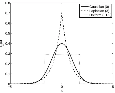
Figure 2.1: Kurtosis excess for several probability distributions, each with zero mean

and unit variance. Shown are a Gaussian distribution (solid, k∗

= 0), a Laplacian

distribution (dashed, k∗

= 3), and a uniform distribution (dotted,k∗

=₋1.2).

kurtosis excess, though this distinction has no bearing on the following discussion.

Figure 2.1 gives a few examples of probability distributions with zero mean and unit

variance but different kurtosis. Note that larger kurtosis corresponds to a taller peak

and heavier tails, which corresponds well with the intuitive definition of sparseness

described above.

Kurtosis is generally described as reflecting either the “peakedness” or the

heav-iness of the tails of fR, and has the convenient property of being invariant both to

shift and scale. In the neural coding literature large values of k are identified with

sparse codes (Olshausen & Field, 1996; Bell & Sejnowski, 1997; Vinje & Gallant,

2000; Willmore & Tolhurst, 2001). This description, however, comes with the caveat

that kurtosis is only appropriately applied to reasonably symmetric, unimodal

dis-tributions such as those obtained from linear filters or artificial neurons (Vinje &

Gallant, 2000; Olshausen & Field, 2004), and not to the one-sided distributions

nec-essarily obtained from real neurons. Vinje and Gallant (2000) alleviate this difficulty

by reflecting their measured neural responses about zero before computing k (that

(25)

bimodal distributions, such as those that may be obtained from neurons involved in

recognition, the meaning of kurtosis remains unclear.

A further challenge confronting the application of kurtosis as a measure of neural

sparseness is its invariance with respect to flipping a distribution about its mean

(because it measures only shape). When evaluated with kurtosis, a neuron that is

highly active, only rarely dropping its firing rate, would be considered just as sparse

as a neuron that is highly inactive, only rarely firing strongly. From an

information-theoretic point of view the two neurons may carry equal information, one conveying

that information by a decrease in firing rate and the other by an increase, but in a

biological context a reasonable sparseness measure should rate the mostly inactive

neuron as much more sparse than the mostly active neuron.

Many of these difficulties stem from the fact that, as a high-order moment, several

disparate factors influence kurtosis and it is difficult at best to capture it intuitively.

Numerous papers in the statistics literature have lamented this difficulty, with

com-ments such as “what do we even mean by kurtosis?” (Bickel & Lehmann, 1975), “there

seems to be no universal agreement about the meaning and interpretation of

kurto-sis”(Moors, 1986), and “there is no agreement on what kurtosis measures”(Ruppert,

1987). Darlington first challenged the traditional interpretation of kurtosis, arguing

that “kurtosis is best decribed not as a measure of peakedness versus flatness, as in

most texts, but as a measure of unimodality versus bimodality” (Darlington, 1970).

This view was later found to fall short of capturing the essence of kurtosis, and the

most precise interpretation is the intuitively unsatisfying one that kurtosis measures

the dispersion of the distribution about the two points µ_±σ (Moors, 1986).

For the reasons outlined above I conclude that, while kurtosis may be a useful

tool for interpreting the sparseness of filters and artificial neurons with symmetric

response distributions, it may not be appropriate for interpreting real neural data.

(26)

obtained, for example, from neurons that fire strongly to some preferred stimulus and

weakly or not at all to other stimuli.

2.1.4 Treves-Rolls Sparseness

Treves and Rolls (1991) present an alternative measure of sparseness more appropriate

for application to neural data. Let fR(r) be the probability density function for the

neuron’s response rates. They defined

a_≡ E[R]

2

E[R2_], (2.3)

that is, the square of the mean response divided by the mean squared response. With

this definition the (dimensionless) sparseness a varies between 0 and 1, and small

values of a correspond to sparse representations. This definition has two convenient

properties. First, in the case of a binary neuron that responds to a stimulus with

probabilityt (and has zero response otherwise),a =t; so indeed, a is the probability

that the neuron responds significantly. Second, from elementary properties of the

mean and variance we can rewrite Equation 2.3 as

a= µ

2

R

µ2

R+σr2

, (2.4)

Thus the sparseness is small if the variance is large compared to the mean (i.e.,

when the neuron has widely separated responses to different stimuli), and large if the

variance is small compared to the mean (i.e., when most responses are very similar).

In addition to being a relatively intuitive generalization of our notion of sparseness

to neurons with continuous rates, a is related to the theoretical storage capacity of

an autoassociative neural network (Tsodyks & Feigel’man, 1988; Treves & Rolls,

(27)

of quantifying the question of how frequently neurons fire “strongly,” but also as a

functionally relevant parameter.

As it is more appropriate than kurtosis when measuring the sparseness of real

neural data, this measure has been used extensively in experimental work (Rolls &

Tovee, 1995; Vinje & Gallant, 2000; Weliky, Fiser, Hunt & Wagner, 2003). In the

remainder of this work I will take this as my primary definition of sparseness.

2.1.5 A Selectivity Index

Working in the context of sparse, invariant neurons in the human medial temporal

lobe (Quian Quiroga et al., 2005), Quian Quiroga and colleagues (2007) propose a

novel threshold-independent index for quantifying the selectivity of neurons. They

first define a function describing the normalized number of responses above a threshold

rT

˜

Sr(rT) =

1 S

S

X

i=1

θ(ri −rT), (2.5)

where θ(x) = 1 for x > 0, θ(x) = 0 for x _≤ 0. Note that if fR(r) is the probability

density function of the response distribution andFR(r) the corresponding cumulative

density function, then for large S S˜r(rT) approaches 1−FR(rT). The area under this

curve (as rT is varied) is

A= 1

M

X

j=1

˜

Sr(rT,j), (2.6)

where rT,j =rmin+j rmax

−rmin

M

defines M equally spaced threshold values between

the minimum and maximum responses rmin and rmax (equivalently one can simply

rescale the responses to lie between 0 and 1). This area will be close to 0.5 for a

uniform distribution of firing rates and much smaller when only a small fraction of

responses are significant. Quian Quiroga and colleagues then define their selectivity

index by

(28)

Consider the case of a binary neuron. If all responses but one are significant, I =

1₋ 2 S−1

S

, so for large S I approaches ₋1. If instead only a single response is

significant, I = 1₋2 _S1

, so for large S I approaches 1.

Assuming a large number of samples and noting the relationship between ˜Sr(rT)

and FR(rT), some algebra yields the relationship

I = 2

rmax−rmin

Z rmax

rmin

F(r)dr₋1, (2.8)

so the selectivity is (in the limit) defined by the cumulative density function of the

response distribution. From this definition it can be seen that any symmetric response

distribution (e.g., Gaussian or uniform) will, in the limit, have I = 0. Thus, like

skewness (which is related to the 3rd _{central moment of a distribution), this measure}

quantifies the asymmetry of the response distribution. Values close to the minimum of

−1 indicate that most responses are clustered near the maximum (the neuron nearly

always responds), values close to the maximum of 1 indicate that most responses are

clustered near the minimum (the neuron rarely responds), and values close to zero

indicate a symmetric response distribution.

As noted by Quian Quiroga et al., this index has a few convenient features.

It is threshold-independent, and captures the selectivity of roughly binary neurons

well and so conforms to our intuitive notion of sparseness. As with any

threshold-independent measure, accurate results depend strongly on a given experiment finding

enough responses to characterize the response distribution well (since no assumptions

are placed on the form of the distribution).

2.1.6 Population versus Lifetime Sparseness

In most discussions of sparse coding, the quantity of interest would more precisely be

(29)

responses over time. This is the sense in which I defined sparseness above. It is

also possible, however, to discuss the sparseness of the responses of a population of

neurons, or the population sparseness. In this case, the relevant sparseness measures

would be the same as defined above, except that the expectations would be taken

across the population of neurons for an individual stimulus rather than across the

universe of stimuli for an individual neuron (perhaps then averaging across all stimuli).

If the neurons’ responses to stimuli are independent and identically distributed,

it is clear from the definitions above that lifetime and population sparseness are

exactly equivalent. Simply speaking, the fraction of stimuli an individual neuron

responds to will be equal to the fraction of neurons that respond to a particular

stimulus. If, however, some neurons participate in many more representations than

others, the population sparseness may be very different than the lifetime sparseness.

Willmore and Tolhurst (2001) investigated this issue by examining the representation

of a set of natural images within several different filtering schemes such as Gabor,

principal components, and independent components filters. They computed both the

population and lifetime sparseness of the responses of each of the filters in each of

these coding systems and found no direct relationship between the two. This should

not be an unexpected result. For example, principle components analysis (PCA)

specifically seeks filters such that a small number of filters code for a large portion of

the input statistics (Hancock, Baddeley & Smith, 1992). A set of PCA filters would

be expected to have a high population sparseness but low average lifetime sparseness,

because a few of the filters have large output much of the time, while many of the

filters are active only rarely.

From an experimental point of view, it is not possible to directly measure the

population sparseness of a given representation—to do so would require recording

from a large enough subset of the entire coding set of neurons to establish the response

(30)

lifetime sparseness, which can be estimated by recording a single neuron’s responses to

a large group of stimuli. Where I make inferences about the population sparseness,

it is under the assumption that the population of neurons under consideration is

homogenous (in the sense of their responses being i.i.d.).

It should be noted that sparseness should properly be defined with respect to a

particular class of “relevant” stimuli. I assume in what follows that the stimulus set is

relevant to the computation performed by the neurons from which we record. In other

work describing experimental results obtained from the human medial temporal lobe

my co-authors and I discuss the potential bias due to choice of stimulus set (Waydo

et al., 2006, and see Chapter 3). Note also that the issues I discuss here are different

than the extreme temporal sparseness observed, for example, in high vocal center

neurons of the zebra finch (Hahnloser et al., 2002; Fiete, Hahnloser, Fee & Seung,

2004). There, neurons appear to encode a time-varying signal (the finch’s song)

using precise spike timing, and “sparseness” refers to the fact that individual neurons

encode their portion of the signal using an extremely small number of spikes. In this

work, I am instead concerned with encoding static signals, and sparseness refers to

how rarely individual neurons will be active (in the case of lifetime sparseness) or

how few neurons will be active simultaneously (in the case of population sparseness).

2.2 Estimation of Sparseness from Neural

Record-ings

As we have seen above, a great deal of work has been done to find an appropriate

quantitative definition of sparseness and to understand how sparseness fits in models

of network performance. Comparatively little attention has been paid to the

prac-tical challenge of how to accurately measure it, the problem to which I now turn.

(31)

while a collection of stimuli is presented to the subject (Young & Yamane, 1992; Rolls

& Tovee, 1995; Vinje & Gallant, 2000; Quian Quiroga et al., 2005; Kreiman et al.,

2006). Due to constraints on experiment duration, the number of stimuli presented

generally varies in the range of about 50–100. The rate of “spontaneous” background

firing, usually of unclear significance (is it noise or signal?), can be significant and

needs to be properly accounted for. In this section I examine two methods for

es-timating representational sparseness from spiking data, direct computation and a

binary model-based approach. My primary contribution is to show that the direct

computation is, in many cases, vulnerable to corruption by noise, particularly if the

underlying code is sparse. I further show that this issue is likely to arise when the

mean noise is large compared to the mean response, regardless of the peak response.

In this regime it is more accurate to apply a binary model using a response threshold

and compute the probability that a neuron fires above that threshold.

This work was performed in collaboration with Christof Koch and Alexander

Kraskov (now at University College London); my contribution was the development

of the probabilistic reasoning about sparseness and the quantification of the biases

inherent in computing sparseness from limited, noisy datasets.

2.2.1 Direct Computation of Sparseness

LetS be the number of stimuli presented andri be the neuron’s response to stimulus

i. The obvious way to estimate a is to calculate the sample mean and the sample

mean square, or, letting ˆa be the estimate ofa,

ˆ a=

1

S

PS

i=1ri

2

1

S

PS

i=1r2i

= r

2

r2, (2.9)

where the bar over a quantity denotes the sample average.

(32)

calcula-tion of the quantity of interest, and so the result needs little interpretacalcula-tion. Secondly,

no underlying assumptions about the neuron’s behavior (i.e., a firing-rate model) are

required—one simply collects the neuron’s responses and plugs them in to Equation

2.9. This second strength, however, may also be a pitfall of this method. If one has a

very sparse neuron for which large responses are rare, one may measure a large

num-ber of responses that are purely noise. Because these responses are all very similar to

one another, Equation 2.9 will erroneously yield a large value. In what follows I will

make this issue more precise.

A fundamental challenge confronting the application of Equation 2.9 is that a is

sensitive to a uniform translation of responses, that is to adding a constant offset to all

responses, such as when taking spontaneous firing into account. For example, consider

a binary neuron with an “off” rate of 0 spikes/s, an “on” rate of 5 spikes/s, and a

firing probability of 5%. The sparseness calculated from Equation 2.3 is a = 5%.

If instead it fires at 6 spikes/s with the same probability and 1 spike/s otherwise,

a = 57%. This is a very different result, but we would argue that the answer to our

basic question (“how often does this neuron respond significantly”) has not changed.

This feature in turn means that the calculation of a can be highly vulnerable

to noise, particularly for very sparse systems. I will here examine the effect of this

vulnerability for a simple model with additive noise. Consider a system in which a

neuron’s response to a stimulus s is the sum of two components, that is

R(s) =X(s) +Y, (2.10)

where X(s) is the deterministic portion of the neuron’s response (that is, X(s) is

some parameterization of the neuron’s tuning curve) and Y is a noise term that is

independent of X. Assuming we choose stimuli randomly from the universe of all

(33)

LetXandY have meansµxandµy and variancesσx2andσ2y, respectively.

Presum-ably in any discussion of sparseness what we are truly interested in is the sparseness

of the distribution of X, which by Equation 2.4 is

a = µ

2

x

µ2

x+σx2

. (2.11)

However, we have only the noisy responses R with which to characterize it. Because

X andY are independent, the response distributionfRhas meanµx+µy and variance

σ2

x+σy2. Applying Equation 2.4, the sparseness of the noisy distribution is then

ˆ

a= (µx+µy)

2

(µx+µy)2+ (σ2x+σy2)

. (2.12)

Comparing Equations 2.11 and 2.12, we see that ˆaapproachesaifµxis large compared

to µy and σy. If this is not the case, ˆa may, in fact, be quite different from the

underlying a that we wish to estimate. Roughly speaking, we have a signal-to-noise

ratio characterized byµx/µy orµx/σy. Even for seemingly low levels of noise, this can

present a significant difficulty. Although the significant responses may be quite large

in comparison to the noise, for a very sparse system we expect themean response to

be small and so ˆa will not accurately reflect a. Note also that only the mean and the

variance of the noise affect Equation 2.12; apart from these parameters the error is

independent of the details of the noise distribution.

Consider the case whereXis a binary distribution, with an “off” rate of 0 spikes/s,

and an “on” rate of 10 spikes/s. The model neuron fires to a random stimulus with

probability a (as we pointed out above, the firing probability of such a neuron is

exactly its sparsenessa). Now add to each response an independent noise component

with mean and standard deviation of 1 spike/s. It would seem in this case that the

signal-to-noise ratio ought to be very favorable: the “on” response is 10 times greater

(34)

0 20 40 60 80 100 0 10 20 30 40 50 60 70 80 90 100 a (%)

estimated a (%)

Binary Gamma ideal

(a) Theoretical sensitivity of sparseness calcula-tion (Equacalcula-tion 2.12) to noise

0 2 4 6 8 10

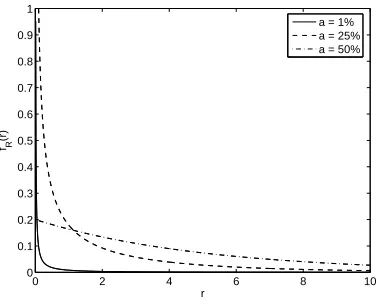
0 0.1 0.2 0.3 0.4 0.5 0.6 0.7 0.8 0.9 1 r fR (r)

a = 1% a = 25% a = 50%

(b) Gamma probability density function for

se-lected values ofa

Figure 2.2: Sensitivity of response sparseness ˆa to noise. Response sparseness is

plotted as a function of the underlying distribution’s sparseness for binary (solid) and gamma (dashed) distribution. High rate for the binary neuron is 10 spikes/s and

scale parameter λ for the gamma neuron is 5, so that both neurons have mean firing

rate 5 spikes/s at a= 1/2. Sparseness is varied by adjusting the firing probability a

for the binary neuron and the shape parameter α for the gamma neuron. The noise

is held constant at 1 spike/s mean and standard deviation.

ˆ

ais between themean responseµxand the mean noiseµy = 1. In this case, the mean

response is 10a, and so if a is even as low as 10% we may run into trouble. Plugging

these numbers into Equations 2.11 & 2.12 reveals that ˆa = 29% for a = 10%, and

ˆ

a= 38% for a= 1%!

While this example used binary model neurons to illustrate noise sensitivity, the

basic issue remains for any response model in which the mean response decreases

with a. For example, consider a neuron whose noiseless firing rates follow a gamma

distribution with shape parameter η and scale parameter λ,

fR(r) =

rη−1_e−r λ

λη_Γ(_η₎ , (2.13)

where Γ(η) is the gamma function. This distribution, depicted in Figure 2.2(b),

is convenient because it has an exponential falloff in rates and an easily tunable

(35)

ηλ. If we fix the scale parameter λ, then the mean rate declines with η and we

have the same bias problem as before. Figure 2.2(a) illustrates this issue for both

the gamma and binary neuron. Plotted is the sparseness estimate ˆa as a function

of the underlying distribution’s sparseness a. Both neurons are parameterized such

that their mean firing rate is 5 spikes/s when a= 1/2. The sparseness of the binary

neuron is adjusted using the response probability a, while that of the gamma neuron

is adjusted using the shape parameterηwhile the scale parameter λis held fixed. For

all levels of sparseness the noise is fixed with mean and standard deviation 1 spike/s.

We see from this figure that the bias due to noise can be substantial. Worse, the

variation of ˆa with a is not even monotonic—the estimated sparseness increases as

the true sparseness becomes very small.

2.2.2 A Binary Model

If we make some a priori assumptions about the underlying rate distribution, we can

generate a few alternative methods for estimating a. In contrast to the direct

calcu-lation, in which the signal-to-noise ratio was that of the means of the response and

noise components, the relevant ratio will be that of the size of the “large” responses to

the noise. We can achieve this by assuming that the neuron responds tosome stimuli

with at least some rate rT, where we pick rT to be our threshold for considering a

response significant. With this threshold we can then treat our neurons as behaving

in a binary fashion, with responses above rT considered “on” and all others “off.” It

is then straightforward to estimate the sparseness simply from the fraction of stimuli

a neuron responds to, or

ˆ a = Sr

S , (2.14)

where S is the total number of stimuli presented and Sr is the number of stimuli

(36)

exactly answers the question of how frequently the neuron responds at a significant

level, as long as we can define a reasonable value for significance. Note that if the

underlying probability of achieving a significant response is a, then Sr follows a

bi-nomial distribution andE[ˆa] =a. This estimate is biased upward by the probability

that an “off” response will be pushed above threshold by noise, so this bias is reduced

by increasing rT. Setting rT too high may, of course, cause significant responses to

be ignored as noise, so the separation between the significant responses and the

back-ground noise is the limiting factor for this method, which is much more favorable

than the difference between the mean response and the background noise in the case

of a sparse distribution.

Continuing with this binary model, I developed a method for determining a range

of sparseness that is consistent with our data, or alternatively the probability

distri-bution of the underlying response probability a. Let fa be the probability density

function of the response probability a. We want to determine fa(α|Sr = sr), the

probability density function for a given the observed number of responses sr. We

place no a priori assumption on a, so we set fa(α) = 1 for 0 ≤ α ≤ 1, that is, a is

equally likely to take on any value between 0 and 1.

At a particular value of a, the number of responses follows the binomial

distribu-tion

P[Sr =sr|a=α] =

  

S

sr

  α

sr₍₁₋_α₎S−sr_. _(2.15)

Bayes’ rule applied to this system gives

(37)

or, solving for the desired distribution,

fa(α|Sr =sr) =

P[Sr =sr|a=α]fa(α)

P[Sr =sr]

=

  

S

sr

  α

sr₍₁₋_α₎S−sr_f

a(α)

R1

0 P[Sr =sr|a=α]fa(α)dα

=

  

S

sr

  α

sr₍₁

−α)S−sr₍_S_{+ 1)}_. _(2.17)

For a given experiment we obtain a curve fa(α) describing the range of plausible

values for the underlying response probability a. Figure 2.3 gives examples of three

such curves derived from three different response patterns with S = 100. It is easy

to check that the peak of this distribution is at α= sr

S, so the most likely value from

this distribution matches the intuitive definition of a for a binary model. We now

have additional information, however, about just how close the true a is likely to be

to our estimate ˆa.

While the imposition of the binary model eliminates the noise sensitivity of the

direct method, it is of course not without challenges of its own. Primary among these

is that the binary model is an approximation of the true behavior that varies in its

accuracy depending on the details of the true firing rate distribution. In some cases

we may have a neuron that responds robustly at a high rate to some stimuli and

much less to others, and so the appropriate choice of threshold is clear. In other

cases, though, a neuron may respond with a wide variety of rates and the resulting

estimate of a based on a binary model will be sensitive to threshold. Obviously this

method sacrifices some of the detail in the neuron’s responses in favor of robustness

to noise.

(38)

sparse-0 5 10 15 20 0

20 40 60 80 100

a (%)

f a

Figure 2.3: Example probability density functions for sparseness (expressed as a percentage of stimuli that evoke a response) computed using Equation 2.17 in three

scenarios in which the number of stimuli presented was S = 100. The solid curve

would be obtained from a neuron for which no significant responses were recorded, while the dashed and dash-dotted curves correspond to neurons for which 1 and 10 significant responses were recorded, respectively. As the number of stimuli shown to the cell approaches the total number of images stored by the network, the density

function will converge to an ever-narrower curve centered at the true sparseness a.

ness of the underlying rate distribution and our estimate ˆa derived from a binary

model. Note that ˆa = P[R _≥ rT], that is, our estimate of a is just the probability

that a response is greater than the threshold rT. The Markov inequality provides

an upper bound for the probability that a positive random variable exceeds some

threshold (Leon-Garcia, 1994). By this inequality,

ˆ

a =P[R_≥rT]≤

E[R] rT

. (2.18)

Applying our additive noise model from above, we have

ˆ

a_≤ µx+µy rT

. (2.19)

(39)

with µ0 =rh, and is approximately true for a gamma neuron with µ0 =λ and small

a. We now have

ˆ

a_≤aµ0 rT

+µy rT

. (2.20)

Here we have an upper bound on ˆa with two convenient features. First, the bias

is equal to µy

rT, the mean noise relative to the threshold, so if our threshold is large

compared to the mean noise the bias is small. Second, the bound decreases with a,

so we are guaranteed that for any choice of threshold a small true a will give us a

small estimate ˆa (provided the mean noise µy is small compared to the threshold).

This bound can also inform our choice ofrT, but some caution is required. Clearly

we would likerT to be significantly larger than the mean noiseµy to reduce the offset

from the noise term. From the first term, the temptation would be to set rT close

to one’s best guess for µ0. The bound given by the Markov inequality may be quite

loose, though, and this approach could result in a significant underestimate of a. A

balance must be struck between making rT as large as possible without getting too

close to µ0.

2.2.3 Simulation Results

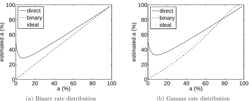
Figures 2.4(a) and (b) depict Monte Carlo simulation results of sparseness

estima-tion with binary and gamma underlying rate distribuestima-tions, respectively. The binary

neuron had an “on” response of 10 spikes/s, while the gamma neuron was tuned to

have the same mean response at each a as the binary neuron. For each neuron I

generated responses toS = 100 stimuli using the appropriate probability distribution

plus Poisson noise with unit (i.e., 1 spike/s) mean and variance. I then estimated

the sparseness of each neuron using both the direct calculation of Equation 2.9 and

the binary model with rT = 5 spikes/s (corresponding to rT = µ0/2 in the above

(40)

0 20 40 60 80 100 0

20 40 60 80 100

a (%)

estimated a (%)

direct binary ideal

(a) Binary rate distribution

0 20 40 60 80 100

a (%)

estimated a (%)

direct binary ideal

(b) Gamma rate distribution

Figure 2.4: Monte Carlo simulation results for sparseness estimation for binary and gamma distribution rate models. Noise was Poisson with 1 spike mean and standard deviation. Solid line is the direct calculation (Equation 2.9); dashed line is the binary calculation with a threshold of 5 spikes/s (Equation 2.14). Dotted line is the ideal of ˆ

a =a (which exactly overlaps the binary calculation in (a)). The number of stimuli

was S = 100, and 1000 neurons were simulated.

type.

In both cases the binary model produced substantially more accurate estimates

than the direct computation, particularly (as predicted) for very sparse distributions.

Because the binary model matched the underlying rate distribution, performance

in that case was nearly perfect. In the case of the gamma distribution, though,

performance was still very good in the sparse regime despite the model mismatch.

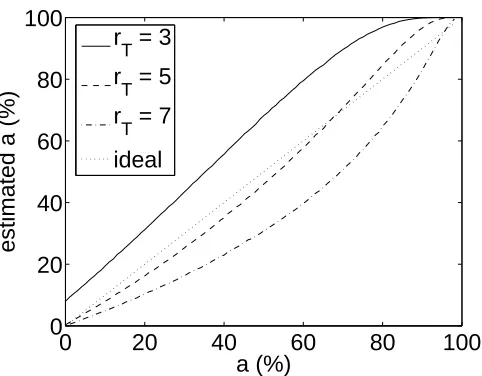
Figure 2.5 shows the effect of the choice of response threshold. Thresholds of

3, 5, and 7 spikes/s are considered with a fixed mean noise level of 1 spike/s. In

the case of the 3 spikes/s threshold, a significant number of “responses” were due to

noise and an overestimate ofaresulted, though this overestimate was still much more

accurate than the direct computation in the sparse regime. The 5 and 7 spikes/s

thresholds both provided estimates close to the truea, and, most importantly, varied

monotonically with a. Figure 2.6 shows the effect of variations in mean noise level

(41)

0 20 40 60 80 100 0

20 40 60 80 100

a (%)

estimated a (%)

r

T = 3

r

T = 5

r

T = 7

ideal

Figure 2.5: Variation of estimated sparseness with threshold. Response thresholds of

3, 5, and 7 spikes/s are considered, with noise level fixed atµy = 1 spike/s. Simulated

responses are drawn from the same gamma distribution as in Figure 2.4(b).

level drew close to the threshold (fixed at 5 spikes/s), many “responses” were due

to noise, resulting in an overestimate of a, but not as severe an overestimate as in

the direct computation case. At noise levels of 1 and 2 spikes/s, the estimates were

close to the true a. The direct computation provided a much worse overestimate of

a, particularly in the sparse regime.

2.2.4 Application to Data

I applied both the binary model and Equation 2.9 to the spiking responses obtained

from 1425 human MTL units from 34 experimental sessions in 11 patients (Quian

Quiroga et al., 2005; Waydo et al., 2006). This data will be discussed in more detail

in the next chapter, but it serves to illustrate the issues I discuss here. Figures 2.7

and 2.8 depict histograms of the results. In Figure 2.7, I calculated for each unit

the percentage of stimuli for which the median response was at least 3 standard

deviations above its background firing rate (for lower thresholds, many “responses”

(42)

0 20 40 60 80 100 0

20 40 60 80 100

a (%)

estimated a (%)

µ_y = 1

µ_y = 2

µ_y = 3

ideal

(a) Binary computation with threshold fixed at

r_T _{= 5 spikes/s}

0 20 40 60 80 100

a (%)

estimated a (%)

µ_y = 1

µ_y = 2

µ_y = 3

ideal

(b) Direct computation

Figure 2.6: Variation of estimated sparseness with mean noise level. Mean noise levels of 1, 2, and 3 spikes/s are considered. Simulated responses are drawn from the same gamma distribution as in Figure 2.4(b).

the choice of threshold). The large majority of these units responded (according to

the 3 standard deviation criterion) to less than 2% of presented stimuli, and the mean

value of this distribution is 1.5%. This is consistent with the qualitative observation

that these units respond in a highly selective manner (Quian Quiroga et al., 2005).

By contrast, Figure 2.8 depicts the sparseness estimate ˆa computed using Equation

2.9 for the same data. In Figure 2.8(a) I applied Equation 2.9 to the raw firing rates,

and the estimate is fairly evenly distributed from 0–100%, with the spike at zero

caused by considering an entirely silent unit to have a sparseness of zero. The mean

value of ˆa computed in this way is 37.8%. In Figure 2.8 I take a common approach

to compensating for noise by subtracting each neuron’s baseline firing rate from its

responses (setting the response to zero in cases where the result is negative). This

improves the results somewhat, with estimates now evenly distributed from 0–40%,

and a mean of 16.6%.

Recalling the example from Section 2.2.1, in which the numbers were motivated

by our experimental data, we see that a true sparseness of 1% can easily lead to a

(43)

0 50 100 0

200 400 600 800 1000 1200

Percent of stimuli responded to

Number of units

Figure 2.7: Histogram of the percentage of stimuli for which the median response was at least three standard deviations above the background rate computed from spiking

responses of 1425 human MTL units. The mean is 1.5%.

0 50 100

0 100 200 300

estimated a (%)

Number of units

(a) Raw firing rates. The mean is 37._8%.

0 50 100

0 100 200 300

estimated a (%)

Number of units

(b) Firing rates with baseline subtracted. The

mean is 16._6%.

(44)

0 200 400 0

200 400 600 800

kurtosis excess

Number of units

Figure 2.9: Histogram of the kurtosis excess for the responses of 1425 human MTL

units. The mean is 29.5.

2.7 and 2.8 are reconciled by the noise sensitivity of Equation 2.9 as described by

Equation 2.12. For this reason, and because it matches much better with the

qual-itative interpretation of the responses as highly sparse (Quian Quiroga et al., 2005)

(that is, the observation of highly selective responses to very few stimuli), I believe the

sparseness value of 1–2% implied by Figure 2.7 is a much more accurate description

of the data.

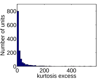
Figure 2.9 is a histogram of the kurtosis excess for the same set of responses. The

kurtosis excess is positive in all but 2% of neurons and has a mean of 29.5, indicating

a sparse response distribution in nearly all cases. Beyond this statement, however,

the kurtosis gives us little quantitative information about neuronal behavior for the

reasons discussed above.

2.2.5 Multiple-Unit Recordings

A limitation of the binary model approach outlined in Section 2.2.2 is that if, for

example, two neurons are presented with the same 100 stimuli and neither responds,

the true sparseness is likely to be much smaller than that implied by the individual

(45)

As in some recent experiments responses are collected simultaneously from up to

several dozen neurons, I extend the binary approach to account for an experiment in

which N neurons are recorded simultaneously while S stimuli are presented. Define

Nrto be the number of neurons that respond above threshold to at least one stimulus,

and Sr to be the number of stimuli that produce a response above threshold in at

least one of these. The derivation of the closed-form joint probability distribution of

Nr and Sr involves solving a recursive relation for the conditional distribution of Sr

given Nr and is described in Appendix A. I simply state the result here:

P[Nr=nr∧Sr =sr|a=α] =

   S sr       N nr  

(1−α)

N S

(₋1)nr

nr X k=1    nr k   (−1)

k

(1₋α)−k

−1sr

. (2.21)

As in the single-neuron case discussed above, we can invert this relationship using

Bayes’ rule to obtain the probability distribution of a given Nr and Sr:

fa(α|Nr=nr∧Sr =sr) =

P[Nr =nr∧Sr =sr|a=α]fa(α)

R1

0 P[Nr=nr∧Sr =sr|a=α]fa(α)dα

. (2.22)

This gives us the probability density function foragiven the results of a full recording

session: Rather than obtaining a single curve for each cell, we now obtain a single

curve for each session that takes into account the presence of cells that did not respond

to any stimulus or that responded to multiple stimuli.

2.2.6 Conclusions

I demonstrated a few of the pitfalls inherent in attempting to estimate sparseness

from experimental spike recordings. In particular, I showed that the most direct way

(46)

where the true sparseness is small. From these developments I emerge with a few

recommendations:

1. If the mean firing rate is on the order of the mean noise level or smaller, the

direct computation will be very error-prone and applying the binary model will

likely lead to much better results.

2. Noise can be problematic for both methods. Repeated exposure to each stimulus

and response averaging should be used to reduce noise levels. Because the noise

is likely to have nonzero mean, however (since these are spiking cells), it will

produce a bias despite this averaging.

3. When applying the binary calculation, the response threshold should be

var-ied over a wide range to examine how estimated sparseness varies with this

(47)

Chapter 3 Experimental Evidence for

Sparseness

In this chapter I describe some of the evidence for sparse coding in biological systems

obtained from electrophysiology experiments. In Section 3.1 I survey results from

recordings taken throughout the visual system. In Section 3.2 I present my own

results (generated in collaboration with Alexander Kraskov, Rodrigo Quian Quiroga,

Itzhak Fried, and Christof Koch) from the human medial temporal lobe (MTL),

which, though not a visual area, sits at the end of the ventral visual pathway and is

linked to associating information across sensory modes and consolidating long-term

memory. Finally, in Section 3.3 I discuss a few relevant findings from the sensory

processing systems of other organisms.

3.1 The Visual System

Vinje and Gallant (2000) assessed the sparseness of the representation of natural

scenes in V1 in awake macaque monkeys. The stimuli were extracted from natural

scenes along simulated eye scan paths, and several patch sizes (1–4 times the classical

receptive field size) were tested to explore the effect of nonclassical receptive field

(nCRF) stimulation on sparseness. The representation became progressively more

Explicit object representation by sparse neural codes

Codes

Stephen Waydo

Acknowledgments

Abstract

Contents

List of Figures

List of Tables

Chapter 1

Overview

1.1

Experimental Motivation

1.2

Outline and Contributions of Thesis

Chapter 2

Quantifying the Sparseness of

Neural Codes

2.1

Sparseness Measures

2.1.1

Notation

2.1.2

Threshold

2.1.3

Kurtosis

2.1.4

Treves-Rolls Sparseness

2.1.5

A Selectivity Index

2.1.6

Population versus Lifetime Sparseness

2.2

Estimation of Sparseness from Neural

Record-ings

2.2.1

Direct Computation of Sparseness

2.2.2

A Binary Model

2.2.3

Simulation Results

2.2.4

Application to Data

2.2.5

Multiple-Unit Recordings

2.2.6

Conclusions

Chapter 3

Experimental Evidence for

Sparseness

3.1

The Visual System