ABSTRACT
BOLDOR, DORIN. Temperature Control of the Continuous Peanut Drying Process Using Microwave Technology. (Under the direction of Timothy H. Sanders and Kenneth R. Swartzel.)
The relationship between dielectric properties of peanuts (Arachis hypogaea L.), thermal and moisture distribution during continuous microwave drying, and automated control of the drying process was investigated. Dielectric properties (ε', ε'') of ground samples of peanut pods and kernels were measured for several densities, temperatures, and moisture contents, in the range of 300 to 3000 MHz. Dielectric mixture equations were used to correlate the dielectric properties with density. The coefficients of quadratic and linear dielectric mixture equations are tabulated for 915 and 2450 MHz, for different temperatures and moisture contents. The values of the dielectric constants (ε') and loss factors (ε'') of bulk peanut pods and kernels were determined by extrapolation of the first and second-order polynomials that relate ε' and ε'' with density. An equation that determines the dielectric properties of bulk peanut pods and kernels as a function of their temperature and moisture content was determined using multiple linear regression.
The temperature profiles obtained from solution of these equations matched the experimental profiles determined using fiber optic temperature probes. The temperature profiles were determined to be dependent on both moisture content and microwave power level. Although the maximum temperature in the microwave applicator was a function of power level only, the rate at which that maximum was attained was a function of dielectric properties and moisture contents of the peanuts. An absolute theoretical determination of moisture content reduction during microwave drying was not possible due to the dependence of dielectric properties on the moisture content. When dielectric properties were assumed independent of moisture content, the theoretical estimations of moisture losses were always lower than the losses determined experimentally, although they were in the same range of values. The surface temperature distribution of the peanut bed measured using infrared pyrometry was well correlated with internal temperature profiles. Thermal imaging demonstrated that the temperature of the peanut bed surface at the exit of the microwave curing chamber was uniformly distributed.
TEMPERATURE CONTROL OF THE CONTINUOUS PEANUT DRYING PROCESS USING MICROWAVE TECHNOLOGY
by
DORIN BOLDOR
A dissertation submitted to the Graduate Faculty of North Carolina State University
in partial fulfillment of the requirements for the Degree of
Doctor of Philosophy
FOOD SCIENCE
BIOLOGICAL AND AGRICULTURAL ENGINEERING
Raleigh 2003
BIOGRAPHY
ACKNOWLEDGEMENTS
I would like to extend my sincere gratitude to Dr. Tim Sanders and Dr. Ken Swartzel for their support and understanding throughout the years we have worked together to complete this project. Their help and advice was invaluable and I will always remember it.
I would like to thank Drs. Andy Hale, Joel Trussell and Michael Drozd too for serving on my Advisory Committee and providing excellent suggestions.
I thank Dr. Josip Simunovic, my good friend and mentor, for the time, effort, resources and humor that supported me for the last 5 years.
I would like to recognize Karl Hedrick, Jack Canady, Gary Cartwright and all the people that work in the Dairy Plant at North Carolina State University for the help they provided during the years I spent in graduate school. Special thanks go to Keith Hendrix and the people working in the USDA-ARS, Market Quality and Handling Research Unit at North Carolina State University for their invaluable help and suggestions regarding the
experimental part of this study. I am also grateful to Elaine Lowell, Susie Kall, Sue Strong, Paula Pharr, Beth McGlamery and Lisa Gordon for their support in fighting bureaucracy. Good times were provided by the Food Engineering crew, Brian Farkas, KP Sandeep, Stephen Sylvia, Jon Bell, Heather Stewart, Koray Palazoglu, Pablo Coronel, Jeff Resch, Qixin Zhong, Ediz Batmaz, and Brian Lloyd.
A special acknowledgement is made to my parents, Dorin and Aurelia Boldor, who always believed in me, even though my father did not live to see my greatest
accomplishments. My sister, Nicoleta Belean, and her family Sorin, Radu and Andrada, together with my aunt Dorina Mesteroiu, and my mother in law Pusa, are the perfect family. I love you all.
TABLE OF CONTENT
LIST OF TABLES……… viii
LIST OF FIGURES………... x
INTRODUCTION………. 1
Justification of research………. 1
Objectives……….. 5
REFERENCES……….. 6
Manuscript 1. Dielectric Properties of In-Shell and Shelled Peanuts at Microwave Frequencies……… 7
ABSTRACT……….. 8
INTRODUCTION………. 9
Dielectric properties of heterogeneous mixtures…….………. 11
MATERIALS AND METHODS……….. 13
RESULTS AND DISCUSSION..………. 15
CONCLUSIONS………... 18
LIST OF SYMBOLS……… 19
REFERENCES………. 20
FIGURE CAPTIONS……… 24
Manuscript 2. Thermal Profiles and Moisture Loss during Continuous Microwave Drying of Peanuts.………. 30
ABSTRACT……….………. 31
INTRODUCTION………. 33
Mathematical development..………. 38
RESULTS AND DISCUSSION………... 48
Simulated results………... 48
Experimental results………. 49
Experimental design 1……….……. 50
Experimental design 2……….. 52
CONCLUSIONS……….. 57
LIST OF SYMBOLS……… 59
REFERENCES………. 60
FIGURE CAPTIONS……… 70
Manuscript 3. Control of Continuous Microwave Drying Process of Farmer Stock Peanuts………... 107
ABSTRACT……….. 108
INTRODUCTION………. 109
Theoretical considerations……… 110
MATERIALS AND METHODS……….. 114
RESULTS AND DISCUSSIONS………. 116
CONCLUSIONS………... 120
LIST OF SYMBOLS……… 121
REFERENCES………. 122
FIGURE CAPTIONS…..………. 126
PROJECT SUMMARY……… 134
LIST OF TABLES
Table 1.1. Values for coefficients and r2 of the quadratic and linear regressions at
915 MHz for kernels……… 22
Table 1.2. Values for coefficients and r2 of the quadratic and linear regressions at
915 MHz for pods……… 22
Table 1.3. Values for coefficients and r2 of the quadratic and linear regressions at
2450 MHz for kernels……….. 23
Table 1.4. Values for coefficients and r2 of the quadratic and linear regressions at
2450 MHz for pods……….. 23
Table 2.1. Locations of the infrared thermocouples ……….………... 64 Table 2.2. Parameters for temperature profiles in Eqn. [2.19] and Figure 2.10 .……. 65 Table 2.3. Parameters for convective and radiative losses in Eqns. [2.35], [2.36] and
Figure 2.11……….. 65
Table 2.4. Parameters for moisture losses in Eqn. [26] and Figure 12………. 65 Table 2.5. Moisture contents (% db) for Virginia type peanuts in three consecutive
passes………... 66
Table 2.6. Moisture contents (% db) for Runner type peanuts in three consecutive
passes………... 66
Table 2.7. Surface temperature distribution for Virginia and Runners type peanuts at the exit from the drying tunnel at 2 power levels and three initial
moisture contents………. 66
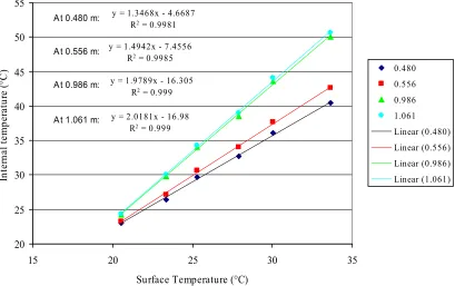
Table 2.8. Relationship between surface and internal temperatures for 11% mc
Runner type peanuts……… 67
Table 2.9. Relationship between surface and internal temperatures for 14% mc
Runner type peanuts……… 67
Table 2.10. Relationship between surface and internal temperatures for 21% mc
Runner type peanuts……… 68
Table 2.11. Relationship between surface and internal temperatures for 33% mc
LIST OF TABLES (cont)
Table 2.12. Moisture losses at 6 power levels……… 69 Table 2.13. Average surface temperature (°C) and standard deviation (°C) for
Runner type peanuts at 4 initial moisture contents undergoing drying at 6
different power levels……….. 69
Table 3.1. Infrared thermocouples locations, grouping and relationship between internal and surface temperature for Runner type peanuts at 33% initial
mc……… 124
Table 3.2. Process parameters for Virginia and Runner type peanuts at 3 initial mc... 124 Table 3.3. Initial tuning parameters for Virginia and Runner type peanuts at 3 initial
mc……… 125
Table 3.4. Initial and optimum tuning parameters and times to get to the set point
LIST OF FIGURES
Figure 1.1. Density dependence of peanut kernels dielectric properties at 18% mc and 30°C at 915 MHz. a. Dielectric constant (ε'); b. Dielectric loss
(ε'')………... 25
Figure 1.2. Density dependence of peanut pods dielectric properties at 23% mc and 30°C at 2450 MHz. a. Dielectric constant (ε'); b. Dielectric loss
(ε'')………... 26
Figure 1.3. Dielectric properties of peanut pods at several moisture contents as a function of frequency at 23°C. a. Dielectric constant (ε'); b. Dielectric
loss (ε'')……… 27
Figure 1.4. Temperature and moisture dependence of dielectric properties of peanut kernels based on the quadratic equations [1.12] and [1.15].
a. Dielectric constant (ε'); b. Dielectric loss (ε'')………. 28 Figure 1.5. Temperature and moisture dependence of dielectric properties of
peanut pods based on the linear equations [1.13] and [1.16].
a. Dielectric constant (ε'); b. Dielectric loss (ε'')………. 29 Figure 2.1. Mechanisms of ionic interaction (Zhong, 2001)………. 73 Figure 2.2. Mechanisms of dipolar interaction (Zhong 2001)………... 74 Figure 2.3. Distribution of the electric field in a transversal section of the TE10
waveguide in the presence of a lossy dielectric at the center of the waveguide. Wave is propagating into the paper. a – waveguide
height, b – waveguide width, w – height of dielectric load……… 75 Figure 2.4. Temperature distribution during microwave drying. The time
coordinate can be changed into distance for a belt moving at constant
speed (Metaxa and Meredith, 1983)……… 76 Figure 2.5. Electric field distribution along a traveling wave applicator. The
distance coordinate is dependent on the time coordinate through the
conveyor belt speed………. 76
Figure 2.6. Microwave generator (a) and the curing chamber (b)………. 77 Figure 2.7. Schematic of the microwave drying system (top) and infrared
thermocouple locations along the waveguide bottom).………... 77 Figure 2.8. Transmitted and reflected power at an impedance mismatch (change
LIST OF FIGURES (cont)
Figure 2.9. Fiber optic probes in peanuts and their location on the conveyor belt… 78 Figure 2.10. Estimated temperature profiles for Runner type peanuts at 21% mc
and 6 power levels………... 79
Figure 2.11. Estimated convective and radiative losses of Runner type peanuts at
21% mc and 2 kW………... 79
Figure 2.12. Estimated moisture losses for Runner type peanuts at 21% mc and 2
kW………... 80
Figure 2.13. Internal temperature (lines) and bed surface temperature (symbols) distributions in Runner type peanuts at 18% initial mc for pods in different locations on the belt. Pod P1 is located closest to the right
wall………. 81
Figure 2.14. Side panels covering cleaning slots on the right side of the drying
chamber………... 81
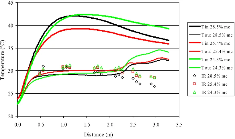
Figure 2.15. Internal temperatures (lines) and surface temperatures (symbols) of
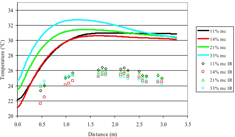
Runner type peanuts at 3 initial mc undergoing drying at 1.2 kW…….. 82 Figure 2.16. Internal temperatures (lines) and surface temperatures (symbols) of
Runner type peanuts at 3 initial mc undergoing drying at 2 kW………. 82 Figure 2.17. Internal temperatures (lines) and surface temperatures (symbols) of
Virginia type peanuts at 3 initial mc undergoing drying at 1.2 kW…… 83 Figure 2.18. Internal temperatures (lines) and surface temperatures (symbols) of
Virginia type peanuts at 3 initial mc undergoing drying at 2 kW……... 83 Figure 2.19. Internal and external temperatures of pods (lines) and bed surface
temperatures (symbols) of Runner type peanuts at 3 initial mc
undergoing drying at 1.2 kW……….. 84 Figure 2.20. Internal and external temperatures of pods (lines) and bed surface
temperatures (symbols) of Runner type peanuts at 3 initial mc
undergoing drying at 2 kW………. 84
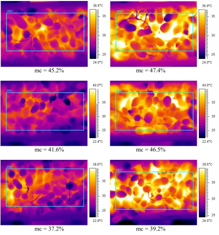
Figure 2.21. Surface temperature distribution at the end of drying of Runner type peanuts at two power levels (1.2 kW – left column, 2 kW – right
LIST OF FIGURES (cont)
Figure 2.22. Surface temperature distribution at the end of drying of Virginia type peanuts at two power levels (1.2 kW – left column, 2 kW – right
column) and indicated initial mc………. 86 Figure 2.23. Internal temperature (lines) and bed surface temperature (symbols)
distributions for Runner type peanuts at 11% initial mc and 6 power
levels……… 87
Figure 2.24. Internal temperature (lines) and bed surface temperature (symbols) distributions for Runner type peanuts at 14% initial mc and 6 power
levels……… 87
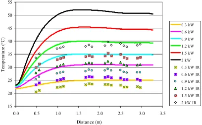
Figure 2.25. Internal temperature (lines) and bed surface temperature (symbols) distributions for Runner type peanuts at 21% initial mc and 6 power
levels……… 88
Figure 2.26. Internal temperature (lines) and bed surface temperature (symbols) distributions for Runner type peanuts at 33% initial mc and 6 power
levels……… 88
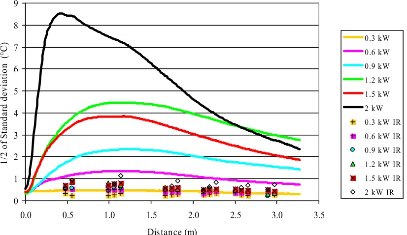
Figure 2.27. Standard deviations for internal temperature (lines) and bed surface temperature (symbols) distributions for Runner type peanuts at 11%
initial mc and 6 power levels………... 89 Figure 2.28. Standard deviations for internal temperature (lines) and bed surface
temperature (symbols) distributions for Runner type peanuts at 14%
initial mc and 6 power levels………... 89 Figure 2.29. Standard deviations for internal temperature (lines) and bed surface
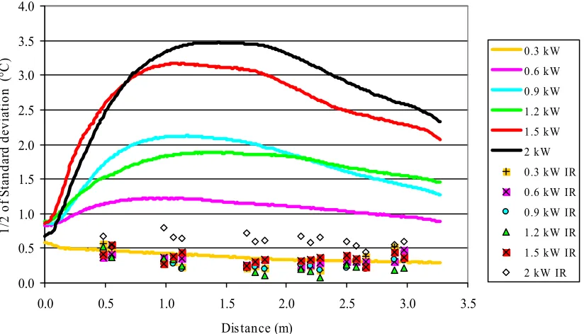
temperature (symbols) distributions for Runner type peanuts at 21%
initial mc and 6 power levels..………. 90 Figure 2.30. Standard deviations for internal temperature (lines) and bed surface
temperature (symbols) distributions for Runner type peanuts at 33%
initial mc and 6 power levels. ………. 90 Figure 2.31. Internal temperatures as function of surface temperature at different
distances in the microwave drying tunnel for Runner type peanuts at
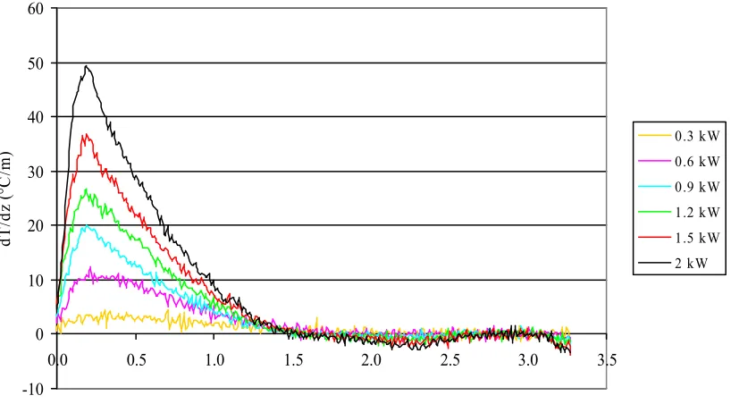
11% initial mc….………... 91 Figure 2.32. First derivative of the internal temperature with respect to distance for
LIST OF FIGURES (cont)
Figure 2.33. First derivative of the internal temperature with respect to distance for Runner type peanuts at 14% initial mc and 6 power levels……… 92 Figure 2.34. First derivative of the internal temperature with respect to distance for
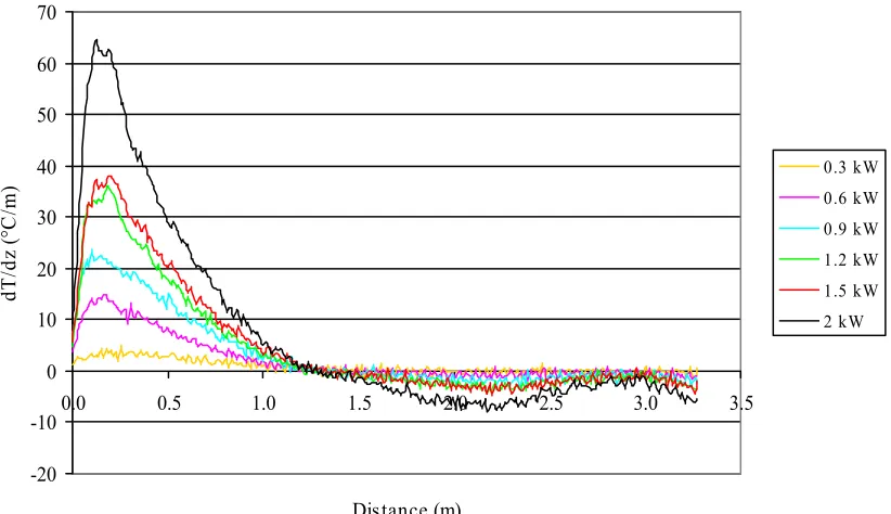
Runner type peanuts at 21% initial mc and 6 power levels... 93 Figure 2.35. First derivative of the internal temperature with respect to distance for
Runner type peanuts at 33% initial mc and 6 power levels……… 93 Figure 2.36. Internal temperature (lines) and bed surface temperature (symbols)
distributions for Runner type peanuts at 0.3 kW and 4 initial mc……... 94 Figure 2.37. Internal temperature (lines) and bed surface temperature (symbols)
distributions for Runner type peanuts at 0.6 kW and 4 initial mc……... 94 Figure 2.38. Internal temperature (lines) and bed surface temperature (symbols)
distributions for Runner type peanuts at 0.9 kW and 4 initial mc…….. 95 Figure 2.39. Internal temperature (lines) and bed surface temperature (symbols)
distributions for Runner type peanuts at 1.2 kW and 4 initial mc……... 95 Figure 2.40. Internal temperature (lines) and bed surface temperature (symbols)
distributions for Runner type peanuts at 1.5 kW and 4 initial mc……... 96 Figure 2.41. Internal temperature (lines) and bed surface temperature (symbols)
distributions for Runner type peanuts at 2 kW and 4 initial mc……….. 96 Figure 2.42. Standard deviations for internal temperature (lines) and bed surface
temperature (symbols) distributions for Runner type peanuts at 0.3 kW and 4 initial mc..………...………... 97 Figure 2.43. Standard deviations for internal temperature (lines) and bed surface
temperature (symbols) distributions for Runner type peanuts at 0.6 kW and 4 initial mc………...………... 97 Figure 2.44. Standard deviations for internal temperature (lines) and bed surface
temperature (symbols) distributions for Runner type peanuts at 0.9 kW
and 4 initial mc………….………...……… 98
Figure 2.45. Standard deviations for internal temperature (lines) and bed surface temperature (symbols) distributions for Runner type peanuts at 1.2 kW
LIST OF FIGURES (cont)
Figure 2.46. Standard deviations for internal temperature (lines) and bed surface temperature (symbols) distributions for Runner type peanuts at 1.5 kW
and 4 initial mc……… 99
Figure 2.47. Standard deviations for internal temperature (lines) and bed surface temperature (symbols) distributions for Runner type peanuts at 2 kW
and 4 initial mc.………... 99 Figure 2.48. First derivative of the internal temperature with respect to distance for
Runner type peanuts at 0.3 kW and 4 initial mc………. 100 Figure 2.49. First derivative of the internal temperature with respect to distance for
Runner type peanuts at 0.6 kW and 4 initial mc………. 100 Figure 2.50. First derivative of the internal temperature with respect to distance for
Runner type peanuts at 0.9 kW and 4 initial mc………. 101 Figure 2.51. First derivative of the internal temperature with respect to distance for
Runner type peanuts at 1.2 kW and 4 initial mc………. 101 Figure 2.52. First derivative of the internal temperature with respect to distance for
Runner type peanuts at 1.5 kW and 4 initial mc………. 102 Figure 2.53. First derivative of the internal temperature with respect to distance for
Runner type peanuts at 2 kW and 4 initial mc……… 102 Figure 2.54. Surface temperature distribution at the end of drying of Runner type
peanuts at 11% initial mc and 6 power levels: a) 0.3 kW, b) 0.6 kW, c) 0.9 kW, d) 1.2 kW, e) 1.5 kW, f) 2.0 kW……… 103 Figure 2.55. Surface temperature distribution at the end of drying of Runner type
peanuts at 14% initial mc and 6 power levels: a) 0.3 kW, b) 0.6 kW, c) 0.9 kW, d) 1.2 kW, e) 1.5 kW, f) 2.0 kW……… 104 Figure 2.56. Surface temperature distribution at the end of drying of Runner type
peanuts at 21% initial mc and 6 power levels: a) 0.3 kW, b) 0.6 kW, c) 0.9 kW, d) 1.2 kW, e) 1.5 kW, f) 2.0 kW……… 105 Figure 2.57. Surface temperature distribution at the end of drying of Runner type
LIST OF FIGURES (cont)
Figure 3.1. Schematic of the microwave drying system (top) and infrared
thermocouple locations along the waveguide (bottom)...………... 127
Figure 3.2. Feedback control loop….……… 127
Figure 3.3. First derivative of the internal temperature with respect to distance in the microwave tunnel for Runner type peanuts at 2 kW and 4 initial mc……… 128
Figure 3.4. Step response of the 16 infrared thermocouples for Runner type peanuts at 52% initial mc……… 128
Figure 3.5. Step response of the six groups of infrared thermocouples for Runner type peanuts at 33% initial mc……… 129
Figure 3.6. Step response of the six groups of infrared thermocouples for Runner type peanuts at 36% initial mc……… 129
Figure 3.7. Step response of the six groups of infrared thermocouples for Runner type peanuts at 52% initial mc……… 130
Figure 3.8. Step response of the six groups of infrared thermocouples for Virginia type peanuts at 22% initial mc……… 130
Figure 3.9. Step response of the six groups of infrared thermocouples for Virginia type peanuts at 26% initial mc……… 131
Figure 3.10. Step response of the six groups of infrared thermocouples for Virginia type peanuts at 44% initial mc……… 131
Figure 3.11. Diagram of the Labview simulation program………. 132
Figure 3.12. Simulation result for initial tuning parameters………... 133
INTRODUCTION
Justification of research
The annual production of peanuts in the United States of America has a field value of more than 1 billion dollars/year (USDA-NASS, 1999b). This figure does not include the existing stocks at farms that exceeds 50 million pounds. The United States is the third largest producer of peanuts in the world, with the first two countries being China and India (USDA-NASS, 1999a).
There are many factors that affect the yield and quality of peanut production. Cultural practices (climatic conditions, crop rotation, land preparation, variety selection, liming, fertilization and mineral nutrition, irrigation, weeds, insect and disease control during growing), maturity at harvesting, and harvesting, curing and storage methods all influence peanut production and quality (Henning et al., 1982). Of these factors, curing (or drying) is the most energy intensive process.
Artificial drying is an energy intensive process and therefore expensive in terms of electrical energy consumed by fans and in terms of fuel consumption for heating the air. A goal of the peanut industry is to reduce energy requirements during drying through use of different methods. Recently developed "green grading" procedure which allow for mixing of different lots before curing are conducing to continuous flow drying procedures. The
reduction in handling will be cost efficient and reduce damage to peanuts.
Current methods used to reduce the cost of artificial drying concentrate on improving energy efficiency of wagon drying methods. This study is focused on application of a new technology for reduction of energy consumption: the use of microwave energy in a
continuous drying applicator. Microwave energy is more efficiently converted into heat when compared with conventional convective drying (Metaxa and Meredith, 1983). Very fast drying rates can be easily achieved which reduces the drying time and thus energy use.
In conventional artificial drying, the driving forces are the temperature and moisture gradient created by heated air blowing through the deep bed of peanuts. The heated air creates a drying front that moves upward through the peanut bed as the drying process progresses (Young et al., 1982). At the pod level, on the outer shell of the pods, heated air creates a front at which the water is heated, vaporized and removed. As drying progresses, this drying front moves inward toward the center of the peanut pod. As the front gets closer to the center of the pod the drying rate decreases as water vapor must diffuse through the peanut in order to be removed from the pod.
The heating takes place volumetrically, and water is heated and vaporized within the whole volume of the peanut pod. The rapidly formed water vapor creates a large pressure gradient that is the driving force in microwave drying.
The energy transfer between the microwave field and material is a function of the dielectric properties of the material. Due to the inherent nature of microwaves, in
conventional microwave ovens, the multiple reflections of the oven walls create standing electric field patterns. These standing waves lead to heating non-uniformities that are
commonly encountered in microwave units and therefore limit the adoption of the technology to a few applications such as tempering of frozen meats. New microwave system designs such as traveling wave applicators create a uniform electric field distribution. A material with uniform dielectric properties running on a conveyor belt at the center of the applicator is exposed to the constant electric field and is uniformly heated.
This study focused on understanding the fundamentals of heating and drying mechanisms of peanuts undergoing continuous microwave drying. There has been little research on continuous microwave drying of peanuts, thus there is a lack of knowledge pertaining to thermal and moisture distribution in peanuts during continuous microwave drying. The influence of dielectric properties on the temperature distribution and moisture reduction in peanuts is not well understood. This study addressed these fundamental issues of continuous microwave drying, as well as a practical application of methods to control the microwave drying process.
The second part covers the theoretical foundation of heat and mass transfer during continuous microwave drying, as well as the experimental work performed to validate the mathematical developments. In this second part, the interpretation of the temperature distributions and moisture reduction data, as related to dielectric properties and initial moisture content of peanuts, and relationship between the internal temperature and the surface temperature of peanut bed are also presented. In the third part relationship between the surface and internal temperature was used to create an effective feedback control algorithm that maintains the temperature at a desired level.
The information and technology created in the study of theoretical and practical aspects of continuous microwave drying can be applied to a large number of agricultural
Objectives
Research objectives were:
- to determine the dielectric properties of peanuts at microwave frequencies and the relationship to temperature and moisture content.
- to determine the influence of peanut dielectric properties and initial moisture content on internal and surface temperature distributions and moisture reduction during continuous microwave drying.
REFERENCES
Henning R.J., Allison A.H. and Tripp L.D. 1982. Cultural Practices. Ch. 5. In Peanut Science and Technology. H.E. Pattee and C.T. Young (Ed.), American Peanut Research and Education Society, Inc., Yoakum, TX.
Metaxa, A.C. and Meredith, R.J. 1983. Industrial Microwave Heating. Peter Peregrinus Ltd., London, UK.
USDA-NASS (United States Department of Agriculture - National Agricultural Statistics Service). 1999a. Agricultural Statistics 1999. United States Government Printing Office. Washington, DC.
USDA-NASS (United States Department of Agriculture - National Agricultural Statistics Service). 1999b. Statistical Highlights of U.S. Agriculture. United States Government Printing Office. Washington, DC.
Manuscript 1. Dielectric Properties of In-Shell and Shelled Peanuts at Microwave Frequencies
D. Boldor1, T.H. Sanders2*, J. Simunovic1
1Department of Food Science
North Carolina State University, Raleigh NC 27695-7624
2 USDA - ARS, Market Quality and Handling Research Unit North Carolina State University, Raleigh, NC 27695-7624
ABSTRACT
Dielectric properties (ε', ε'') of ground samples of peanut (Arachis hypogaea L.) pods and kernels were measured for several densities, temperatures, and moisture contents, in the range of 300 to 3000 MHz. Dielectric mixture equations were used to correlate the dielectric properties with density. The coefficients of quadratic and linear dielectric mixture equations are tabulated for 915 and 2450 MHz, for different temperatures and moisture contents. The values of the dielectric constants (ε') and loss factors (ε'') of bulk peanut pods and kernels were determined by extrapolation of the first and second-order polynomials that relate ε' and
ε'' with density. An equation that determines the dielectric properties of bulk peanut pods and kernels as a function of their temperature and moisture content was determined using
multiple linear regression.
INTRODUCTION
Dielectric properties (ε', ε'') of materials characterize their interaction (transmittance, absorbance, and reflection) with electric fields, and implicitly with electromagnetic waves, including those in the microwave region. Dielectric theory and dielectric properties of materials have been studied in detail for many years (von Hippel, 1954; Birks, 1967) and a comprehensive review has been recently published (Neelakanta, 1995). Dielectric properties also characterize the ability of the material to dissipate electromagnetic energy as heat (Nelson, 1992) according to:
P = σ E2 = 2 π f ε0ε'' E2 [1.1]
Microwave drying and roasting are two major agricultural related processing applications in which the knowledge of the dielectric properties of various agricultural commodities is important. Many commodities have their dielectric properties compiled in extensive studies (Nelson, 1973; ASAE, 2000b).
Whitney and Porterfield (1967) measured the dielectric properties of Starr peanuts at frequencies up to 50 MHz. While some of their results are similar to those reported by other researchers, their analysis has been criticized for large errors in high moisture peanuts and methods used in measurement (Nelson, 1973). Also the dielectric properties in the
For biological materials (non ferromagnetic) the dielectric properties of interest are the dielectric constant (ε') and the dielectric loss (ε''), which relate to the complex permittivity ε
through the relationship (Nelson, 1978):
ε = ε' – j ε'' [1.2]
Where ε' and ε'' are relative to the permittivity of free space (vacuum) ε0.
Free air has a similar permittivity to a vacuum (no loss and the same storage ability), therefore it can be approximated as:
εair = 1 – j 0 [1.3]
Two other properties of interest in microwave processing of biological materials are conductivity (σ) and loss tangent (tan δ):
σ = ωε0 ε'' [1.4]
tan δ = ε''/ε' [1.5]
The permittivity of materials varies with frequency (von Hippel, 1954; Lawrence et al., 1990; Neelakanta, 1995), and for pure polar materials it can be expressed using Debye’s equation (von Hippel, 1954):
τ + − + = ∞ ∞ ω j 1 ε' ε' ε'
ε s ;
2 2 s τ ω 1 ε' ε' ε' ε' + − + = ∞ ∞ ;
(
)
2 2 s τ ω 1 τ ω ε' ε' ' ε' + −= ∞ [1.6]
For non-pure polar materials an extension of Debye’s equation (Cole-Cole equation) is used (Nelson, 1973):
α 1 s τ) ω (j 1 ε' ε' ε' ε ∞− ∞ + − +
The general equations presented so far cannot be used in evaluating the dielectric
constant and dielectric loss of peanuts as they are not pure polar materials, they have multiple layers (in the case of in-shell peanuts) and they form a heterogeneous mix with the air that surrounds them.
Dielectric properties of heterogeneous mixtures
In microwave processing, the influence of the dielectric properties depends on the amount of mass interacting with the electromagnetic field. Therefore, given that the total volume is constrained by the microwave cavity, the density (mass/unit volume) will have an effect on dielectric properties. This is especially notable with particulate dielectrics such as pulverized or granular materials (Nelson, 1983; Nelson, 1992). The influence of bulk density on dielectric properties has been studied in detail and equations have been developed that can be applied to heterogeneous mixtures (van Beek, 1967; Tinga and Voss, 1973).
∑
+ − −+ =
i i 2
2 2 mix 1) (ε A 1 1 ε v 3 1 1
ε ; if v2 < 0.1 [1.8]
∑
+ −−+ =
i 1 i 2 1
2 1 2
mix ε A (ε ε )
1) (ε ε v 3 1 1
ε ; for any v2 [1.9]
Where for prolate spheroids:
− + − + − − = 2 1 2 i i i i 2 3 2 i i i i 2 i i
i b 1
a b a ln 1 b a b a 1 b a 1
An alternative approach for determining the dielectric properties of particulate and pulverized materials has been developed throughout the years. It is based on the observation that the dielectric constant and dielectric loss for granular and pulverized samples depend on density according to the following formulas (Nelson, 1983; Nelson et al., 1991; Nelson, 1992):
ε' = 1 + A1 ρ + A2 ρ2 [1.11]
(ε')1/2 = m1 ρ+ 1 [1.12]
(ε')1/3 = m3 ρ+ 1 [1.13]
ε'' = B1 ρ + B2 ρ2 [1.14]
(ε'' + e)1/2 = m2 ρ + (e)1/2 [1.15]
where: e = B12/(4*B2) [1.16]
These equations are similar with the complex refractive index mixture equation [1.17] (Kraszewski, 1977; Nelson et al., 1991) and the Landau and Lifshitz, Looyenga equation [1.18] (van Beek, 1967)
;
2 1 1 v
v ; ε v ε v
εmix = 1 1 + 2 2 = − [1.17]
;
2 1 1 v v ; ε v ε v ε 3 1 2 2 3 1 1 1 3 1
mix = + = − [1.18]
MATERIALS AND METHODS
Field dried peanuts were shipped from USDA – ARS National Peanut Research Laboratory in Dawson, Georgia in August 2002 to North Carolina State University. They were separated into 4 different samples. The first sample was stored in a cooler at 8°C, while the others were dried on an air blower in three stages, to reach a total of four different
moisture contents. The moisture content of each sample was determined according to ASAE Standards (ASAE, 2000a). Each sample was subsequently divided into two separate samples, out of which one was shelled in order to determine the dielectric properties of both in-shell and shelled peanuts. In addition to bulk moisture content of the samples, the moisture content of each sample undergoing dielectric properties measurements was measured by collecting a small sample after the dielectric measurement.
The peanut samples were sealed in quarter size plastic bags and left to equilibrate their moisture content for 24 hours in refrigerator at 4°C. After equilibration the bags were
For temperatures above room temperature, the jars were held in water baths for a few hours, until an extra jar with temperature sensor at the geometric center filled at the highest density was determined to be at thermal equilibrium with the water bath.
Dielectric properties were measured with a HP Network Analyzer 8753C (Hewlett-Packard, Palo Alto, CA) using the open-ended coaxial probe method adapted from Nelson and Bartley (2000) and Engelder and Buffler (1991), in a 361 point frequency sweep from 300 MHz to 3 GHz. The network analyzer was controlled by Hewlett-Packard 85070B dielectric kit software (Hewlett-Packard, Palo Alto, CA) and calibrated using the 3-point method (short-circuit, air and water at 25°C).
The least square method (Milton and Arnold, 1995) was used in Matlab (The
Mathworks, Inc., Natick, MA) to determine the coefficients of regression (A1, A2, B1, B2, m1, m2, m3, e) and coefficients of determination (r2) for ε' and ε'' as a function of density for all 361 points in the frequency sweep. The method was used for both first-order and second-order polynomials according to equations [1.11] - [1.16] as described by Nelson (1984). Dielectric properties of in-shell and shelled peanuts at nominal bulk density for all moisture contents and temperatures tested were determined afterward using dielectric mixture equations [1.11] to [1.15] in Microsoft Excel XP (Microsoft Corp., Redmond, WA). The equations that relate the dielectric properties of peanut pods and kernels to their moisture content and absolute temperature were obtained by performing multiple linear regression on the logarithmic transforms of the data:
RESULTS AND DISCUSSION
The FCC regulates the use of frequencies of the electromagnetic spectrum in the US, and the two frequencies reserved for food uses are 915 MHz and 2.45 GHz. Most of the results presented here are at these two frequencies.
The dielectric properties of ground pods and kernels as a function of density are displayed in Figures 1.1 and 1.2. The density dependence of the dielectric properties (ε' and
ε'') of ground peanuts is similar to those obtained for other agricultural commodities (Nelson and You, 1989). As the density increases, the dielectric properties increase for both ground kernels and ground pods. The dependence was determined using equations [1.11] to [1.17] with very good results. In general the quadratic equations [1.11] and [1.14] give better estimates of the dielectric properties (r2 > 0.9) than linear equation [1.12], [1.13] and [1.15] respectively. The coefficients for quadratic and linear predictive equations ([1.11] to [1.16]) as a function of density for peanuts at various temperatures and moisture contents are presented in Tables 1.1 through 1.4.
Since deviations from the equation [1.14] are noticed even in lower moisture peanuts, the authors hypothesize that in addition to increased water mobility, oil extraction from peanuts also has a previously unaccounted effect on the density dependence of dielectric properties. The extraction of oil is caused by a combination of the grinding process, the pressure applied to create a high density mixture, and the higher temperatures. Ground peanuts change from a heterogeneous mixture of solids and air to a mixture of solids, oil, and air, and the linear dielectric mixture equations [1.11] – [1.16] do not accurately represent the system. In this case the quadratic equations [1.11] and [1.14] prove to be valuable tools in estimating the dielectric properties of peanuts at high temperatures and moisture content.
Dielectric properties of Georgia Green peanut kernels as a function of frequency at 23°C and all four moisture contents are presented in Figure 1.3. While the dielectric properties decrease with frequency, they increase as the moisture content increases up to 33%, and afterward decrease at 39% mc. This effect was previously noticed in potatoes and explained by Mudgett (1995) by a dilution of dissolved salts by the extra free water. The dielectric mixture theory equations [1.11] to [1.16] were used subsequently to determine the dielectric properties of bulk peanuts at different moisture contents and densities (Figures 1.4 and 1.5).
The authors assume that at temperatures above those studied in this paper, the dielectric loss of peanuts will increase significantly according to the microwave thermal runaway effect (Rosenthal, 1992).
The multiple linear regression performed on the logarithmic transforms of the data (equations [1.19] and [1.20]) gives the following relationship of the dielectric properties of the peanuts with their moisture content and temperature:
Kernels at 915 MHz: ε' = 102.6840 * T(K)-0.5262 * mc0.8870 r2 = 0.83 [1.21]
ε''= 105.5882 * T(K)-1.8323 * mc1.3083 r2 = 0.84 [1.22] Kernels at 2450 MHz: ε' = 102.1730 * T(K)-0.3401 * mc0.8562 r2 = 0.85 [1.23]
ε''= 107.8072 * T(K)-2.7511 * mc1.3483 r2 = 0.86 [1.24] Pods at 915 MHz: ε' = 100.7776 * T(K)0.2299 * mc1.2642 r2 = 0.93 [1.25]
ε''= 103.1577 * T(K)-0.7181 * mc2.4603 r2 = 0.93 [1.26] Pods at 2450 MHZ: ε' = 100.5638 * T(K)0.2843 * mc1.1614 r2 = 0.94 [1.27]
CONCLUSIONS
LIST OF SYMBOLS
ai, bi – major and minor axis of the prolate spheroids; m
Ai – depolarizing factor
A1, A2 – regression coefficients of dielectric constant quadratic equations
B1, B2 – regression coefficients of dielectric loss quadratic equations
c1, c2, c3 – coefficients of regression equation
e – regression constant E – electric field; V/m f – frequency; Hz j – (-1)1/2
m1, m2, m3 – regression coefficients for linear equations
mc – moisture content dry basis; % P – power absorbed per unit volume; W/m3
tan δ – loss tangent (tan δ = ε''/ε' = σ/ωε0ε') T – absolute temperature; K
v1 – volume fraction of the continuous phase (air)
v2 – volume fraction of the dispersed phase (solid)
α – spread of relaxation times; α∈[0,1] δ − phase of a complex number
ε – relative complex permittivity or relative complex dielectric constant ε0 – dielectric constant of the vacuum = 8.854 10-12 Far/m
ε1 – relative dielectric constant of the continuous phase (air)
ε2 – relative dielectric constant of the dispersed phase (solids)
εmix – relative dielectric constant of a mixture
ε∞ – relative dielectric constant as ω goes to infinity
1
ε – mean value permittivity around a spheroid particle ε' – relative electric constant or storage factor
εs' – relative static dielectric constant (at ω = 0)
ε'' – relative dielectric loss or loss factor σ – conductivity; siemen/m
REFERENCES
ASAE Standards. 2000a. Moisture Measurement – Peanuts. ASAE S410.1 DEC97. ASAE, 2950 Niles Road, St. Joseph, MI 49085-9659 USA
ASAE Standards. 2000b. Dielectric Properties of Grain and Seed. ASAE D293.2 DEC99. ASAE, 2950 Niles Road, St. Joseph, MI 49085-9659 USA
Birks, J.B. 1967. Progress in Dielectrics. CRC Press, Cleveland, OH.
Engelder, D.S., Buffler, C.R. 1991. Measuring Dielectric Properties of Food Products at Microwave Frequencies. Microwave World, 12(2):2-11
Kent, M. 1977. Complex Permittivity of Fish Meal: A General Discussion of Temperature, Density and Moisture Dependence. Journal of Microwave Power, 12(4):341-345 Kim, Y.-R., Morgan, M.T., Okos, M.R., Stroshine, R.L. 1998. Measurement and Prediction
of Dielectric Properties of Biscuit Dough at 27 MHz. Journal of Microwave Power and Electromagnetic Energy, 33(3):184-194
Kraszewski, A. 1977. Prediction of the Dielectric Properties of Two-Phase Mixtures. Journal of Microwave Power, 12(3):215-222
Lawrence, K.C., Nelson, S.O., Kraszewski, A. 1990. Temperature Dependence of the Dielectric Properties of Wheat. Transactions of the ASAE, 33(2):535-540
Lawrence, K.C., Nelson, S.O., Kraszewski, A. 1992. Temperature Dependence of the Dielectric Properties of Pecans. Transactions of the ASAE, 35(1):251-255
Milton, J.S., Arnold, J.C. 1995. Introduction to Probability and Statistics: Principles and applications for engineering and the computing sciences. 3rd Ed. Irwin McGraw-Hill, New York, NY.
Mudgett, R.E. 1995. Electrical Properties of Foods. In Engineering Properties of Foods. 2nd Ed. Edited by Rao, M.A., Rizvi, S.S.H. Marcel Dekker, Inc. New York, NY.
Neelakanta, P.S.1995. Handbook of Electromagnetic Materials: monolithic and composite versions and their applications. CRC Press LLC,Boca Raton, FL.
Nelson, S.O. 1973. Electrical Properties of Agricultural Products (A Critical Review).
Transactions of the ASAE, 16(2):384-400
Nelson, S.O. 1981. Frequency and Moisture Dependence of the Dielectric Properties of Chopped Pecans. Transactions of the ASAE, 24(6):1573-1576
Nelson, S.O. 1983. Observations on the Density Dependence of Dielectric Properties of Particulate Materials. Journal of Microwave Power, 18(2):143-152
Nelson, S.O. 1984. Density Dependence of the Dielectric Properties of Wheat and Whole-Wheat Flour. Journal of Microwave Power, 19(1):55-64
Nelson, S.O., You, T.-S. 1989. Microwave Dielectric Properties of Corn and Wheat Kernels and Soybeans. Transactions of the ASAE, 32(1):242-249
Nelson, S.O., Kraszewski, A., You, T.-S. 1991. Solid and Particulate Material Permittivity Relationships. Journal of Microwave Power and Electromagnetic Energy, 26(1):45-51 Nelson, S.O. 1992. Correlating Dielectric Properties of Solid and Particulate Samples
Through Mixture Relationships. Transactions of the ASAE, 35(2):625-629
Nelson, S.O., Bartley, P.G. 2000. Measuring Frequency – and Temperature – Dependent Dielectric Properties of Food Materials. Presentation at the 2000 ASAE Annual International Meeting, Paper No. 006096. ASAE, 2950 Niles Road, St. Joseph, MI 49085-9659 USA
Rosenthal, I. 1992. Electromagnetic Radiation in Food Science. Springer-Verlag Berlin. Tinga, W.R, Voss, A.G. 1973. Generalized approach to multiphase dielectric mixture theory.
Journal of Applied Physics, 44(9):3897-3902
van Beek, L.K.H. 1967. Dielectric Behaviour of Heterogeneous Systems. In Progress in Dielectrics, edited by Brick, J.B. CRC Press, Cleveland, OH.
von Hippel, A.R. 1954. Dielectric Materials and Application. The Technology Press of M.I.T., John Wiley & Sons, Inc., New York, NY and Chapman & Hall, Ltd., London, UK
Whitney, J.D., Porterfield, J.G. 1967. Dielectric Properties of Peanuts. Transactions of the ASAE, 10(1):38-39,42.
Table 1.1. Values for coefficients and r2 of the quadratic and linear regressions at 915 MHz for kernels MC (%), ρ (kg/m3) 18%, (628 kg/m3) 23% (654.6 kg/m3)
Temp (°C) 23 30 40 50 23 30 40 50
ε' = A2ρ2+A1ρ+1 A2 1.135E-5 9.150E-6 8.530E-6 1.138E-5 1.670E-5 1.450E-5 1.911E-5 1.680E-5 A1 -9.280E-4 1.029E-3 1.392E-3 -7.700E-4 -3.672E-3 -4.242E-3 -6.571E-3 -4.868E-3 r2 0.960 0.849 0.756 0.897 0.994 0.956 0.988 0.981
ε'1/2 = m1ρ+1 m1 2.059E-3 2.131E-3 2.106E-3 2.091E-3 2.354E-3 1.929E-3 2.144E-3 2.145E-3 r2 0.837 0.788 0.703 0.789 0.861 0.798 0.770 0.814
ε'1/3 = m3ρ+1 m3 1.151E-3 1.187E-3 1.173E-3 1.166E-3 1.279E-3 1.073E-3 1.173E-3 1.177E-3 r2 0.872 0.815 0.725 0.822 0.904 0.846 0.808 0.859
ε'' = B2ρ 2+B1ρ B2 3.025E-6 2.243E-6 2.214E-6 3.870E-6 4.609E-6 3.638E-6 5.207E-6 4.819E-6 B1 1.730E-4 5.590E-4 5.540E-4 -7.500E-4 -5.840E-4 -8.920E-4 -1.740E-3 -1.640E-3 r2 0.985 0.916 0.787 0.920 0.985 0.892 0.937 0.962
(ε''+e)1/2 = m2ρ+e1/2 e 2.481E-3 3.484E-2 3.468E-2 3.634E-2 1.851E-2 5.469E-2 1.453E-1 1.396E-1 m2 1.740E-3 1.494E-3 1.475E-3 1.421E-3 1.782E-3 1.279E-3 1.259E-3 1.192E-3 r2 0.980 0.930 0.798 0.839 0.971 0.845 0.798 0.799 MC (%), ρ (kg/m3) 33%, (715.3 kg/m3) 39% (751.3 kg/m3)
Temp (°C) 23 30 40 50 23 30 40 50
ε' = A2ρ2+A1ρ+1 A2 1.327E-5 1.534E-5 4.698E-6 -5.909E-6 3.961E-6 4.292E-6 1.400E-6 3.193E-6 A1 2.725E-3 2.481E-5 1.001E-2 1.724E-2 -1.962E-2 1.159E-2 -1.200E-4 9.115E-3 r2 0.926 0.958 0.952 0.974 0.936 0.985 0.983 0.970
ε'1/2 = m1ρ+1 m1 3.014E-3 3.241E-3 3.055E-3 2.819E-3 2.600E-3 3.268E-3 2.715E-3 2.749E-3 r2 0.900 0.957 0.954 0.278 0.611 0.928 0.933 0.895
ε'1/3 = m3ρ+1 m3 1.561E-3 1.665E-3 1.589E-3 1.491E-3 1.360E-3 1.697E-3 1.433E-3 1.456E-3 r2 0.925 0.963 0.909 -0.235 0.658 0.781 0.976 0.744
ε'' = B2ρ 2+B1ρ B2 5.191E-6 5.712E-6 2.471E-6 -2.856E-6 1.356E-5 2.436E-6 4.860E-6 1.130E-6 B1 2.800E-4 4.380E-4 2.685E-3 6.615E-3 -6.608E-3 3.261E-3 -1.380E-4 2.996E-3 r2 0.948 0.909 0.954 0.926 0.825 0.971 0.949 0.973
(ε''+e)1/2 = m2ρ+e1/2 e 3.770E-3 8.387E-3 7.293E-1 -3.830E+0 8.054E-1 1.092E+0 9.820E-4 1.986E+0 m2 2.263E-3 2.392E-3 1.568E-3 N/A 1.323E-3 1.560E-3 2.129E-3 1.063E-3 r2 0.952 0.889 0.959 N/A 0.529 0.969 0.937 0.972
Table 1.2. Values for coefficients and r2 of the quadratic and linear regressions at 915 MHz for pods MC (%), ρ (kg/m3) 18% (332 kg/m3) 23% (338.6 kg/m3)
Temp (°C) 23 30 40 50 23 30 40 50
ε' = A2ρ2+A1ρ+1 A2 2.172E-5 1.854E-5 1.095E-5 -3.300E-7 1.478E-5 3.790E-6 1.412E-5 5.590E-6 A1 -5.026E-3 -4.582E-3 -8.000E-6 7.601E-3 -5.250E-4 5.782E-3 -2.770E-4 4.401E-3 r2 0.978 0.973 0.933 0.984 0.999 0.989 0.962 0.887
ε'1/2 = m1ρ+1 m1 1.673E-3 1.753E-3 1.889E-3 2.343E-3 2.270E-3 2.387E-3 2.247E-3 2.290E-3 r2 0.647 0.685 0.816 0.845 0.893 0.976 0.880 0.865
ε'1/3 = m3ρ+1 m3 1.005E-3 1.033E-3 1.107E-3 1.354E-3 1.300E-3 1.367E-3 1.289E-3 1.316E-3 r2 0.687 0.735 0.843 0.703 0.931 0.924 0.922 0.830
ε'' = B2ρ 2+B1ρ B2 4.603E-6 3.965E-6 3.043E-6 -2.371E-6 4.200E-6 8.860E-7 4.257E-6 1.328E-6 B1 -2.000E-4 -5.400E-4 -2.800E-5 3.349E-3 -7.400E-5 1.638E-3 -3.000E-4 1.230E-3 r2 0.963 0.999 0.981 0.988 0.993 0.902 0.925 0.843
(ε''+e)1/2 = m2ρ+e1/2 e 2.094E-3 1.810E-2 6.250E-5 -1.183E+0 3.270E-4 7.571E-1 5.308E-3 2.849E-1 m2 1.937E-3 1.475E-3 1.711E-3 N/A 1.981E-3 9.400E-4 1.781E-3 1.151E-3 r2 0.949 0.933 0.978 N/A 0.991 0.892 0.914 0.814 MC (%), ρ (kg/m3) 33% (366.6 kg/m3) 39% (384.3 kg/m3)
Temp (°C) 23 30 40 50 23 30 40 50
ε' = A2ρ2+A1ρ+1 A2 2.289E-5 4.469E-5 4.137E-5 2.412E-5 2.942E-5 4.897E-5 3.889E-5 2.720E-6 A1 2.235E-3 -8.431E-3 -8.261E-3 3.665E-3 6.150E-3 -1.083E-2 -3.913E-3 1.391E-3 r2 0.838 0.918 0.775 0.965 0.735 0.991 0.998 0.972
ε'1/2 = m1ρ+1 m1 3.723E-3 4.110E-3 3.823E-3 4.082E-3 4.654E-3 4.054E-3 4.207E-3 3.700E-3 r2 0.836 0.867 0.746 0.969 0.691 0.848 0.904 0.842
ε'1/3 = m3ρ+1 m3 1.961E-3 2.133E-3 2.003E-3 2.130E-3 2.388E-3 2.096E-3 2.724E-3 1.722E-3 r2 0.868 0.921 0.800 0.975 0.710 0.892 0.937 0.655
ε'' = B2ρ 2+B1ρ B2 6.894E-6 1.995E-5 2.082E-5 1.600E-5 9.772E-6 1.824E-5 1.903E-5 2.249E-6 B1 1.451E-3 -4.860E-3 -6.250E-3 -1.970E-3 3.243E-3 -3.860E-3 -3.470E-3 4.774E-3 r2 0.754 0.870 0.696 0.964 0.783 0.988 0.996 0.968
Table 1.3. Values for coefficients and r2 of the quadratic and linear regressions at 2450 MHz for kernels MC (%), ρ (kg/m3) 18% ( 628 kg/m3) 23% (654.6 kg/m3)
Temp (°C) 23 30 40 50 23 30 40 50
ε' = A2ρ2+A1ρ+1 A2 8.384E-6 6.937E-6 6.663E-6 8.640E-6 1.327E-5 1.124E-5 1.491E-5 1.293E-5 A1 5.930E-4 2.079E-3 2.129E-3 5.450E-4 -1.811E-3 -2.115E-3 -3.948E-3 -2.236E-3 r2 0.949 0.843 0.763 0.899 0.996 0.960 0.989 0.978
ε'1/2 = m1ρ+1 m1 1.939E-3 2.027E-3 1.991E-3 1.964E-3 2.227E-3 1.867E-3 2.049E-3 2.097E-3 r2 0.870 0.810 0.731 0.828 0.896 0.853 0.827 0.875
ε'1/3 = m3ρ+1 m3 1.094E-3 1.137E-3 1.118E-3 1.106E-3 1.221E-3 1.046E-3 1.132E-3 1.158E-3 r2 0.899 0.833 0.751 0.858 0.936 0.898 0.869 0.919
ε'' = B2ρ 2+B1ρ B2 3.220E-6 2.720E-6 3.051E-6 4.272E-6 5.201E-6 4.109E-6 5.765E-6 5.201E-6 B1 -4.960E-4 -2.990E-5 -5.570E-4 -1.550E-3 -1.475E-3 -1.519E-3 -2.631E-3 -2.334E-3 r2 0.988 0.882 0.765 0.897 0.986 0.914 0.951 0.966
(ε''+e)1/2 = m2ρ+e1/2 e 1.911E-2 8.098E-5 2.540E-2 1.406E-1 1.046E-1 1.404E-1 3.001E-1 2.618E-1 m2 1.403E-3 1.616E-3 1.264E-3 9.930E-4 1.412E-3 1.021E-3 9.310E-4 9.070E-4 r2 0.940 0.896 0.636 0.620 0.862 0.745 0.631 0.644 MC (%), ρ (kg/m3) 33%, (715.3 kg/m3) 39% (751.3 kg/m3)
Temp (°C) 23 30 40 50 23 30 40 50
ε' = A2ρ2+A1ρ+1 A2 9.962E-6 1.312E-5 2.738E-6 -6.565E-6 3.352E-5 2.596E-6 1.139E-5 1.139E-6 A1 3.966E-3 2.713E-3 1.037E-2 1.671E-2 -1.606E-2 1.172E-2 1.118E-3 9.965E-3 r2 0.920 0.969 0.956 0.989 0.935 0.961 0.988 0.981
ε'1/2 = m1ρ+1 m1 2.801E-3 3.019E-3 2.873E-3 2.653E-3 2.430E-3 3.093E-3 2.568E-3 2.615E-3 r2 0.915 0.967 0.938 -0.036 0.631 0.889 0.953 0.837
ε'1/3 = m3ρ+1 m3 1.470E-3 1.569E-3 1.510E-3 1.416E-3 1.288E-3 1.620E-3 1.368E-3 1.396E-3 r2 0.935 0.973 0.869 -0.711 0.681 0.734 0.986 0.628
ε'' = B2ρ 2+B1ρ B2 4.677E-6 5.228E-6 2.019E-6 -1.995E-6 1.251E-5 2.335E-6 4.265E-6 1.666E-6 B1 1.840E-4 9.100E-5 2.324E-3 4.980E-3 -6.555E-3 2.351E-3 -4.590E-4 1.717E-3 r2 0.930 0.943 0.941 0.963 0.884 0.974 0.968 0.944
(ε''+e)1/2 = m2ρ+e1/2 e 1.800E-3 3.940E-4 6.687E-1 -3.107E+0 8.590E-1 5.920E-1 1.235E-2 4.423E-1 m2 2.144E-3 2.290E-3 1.417E-3 N/A 1.108E-3 1.527E-3 1.798E-3 1.291E-3 r2 0.935 0.933 0.948 N/A 0.507 0.970 0.952 0.938
Table 1.4. Values for coefficients and r2 of the quadratic and linear regressions at 2450 MHz for pods MC (%), ρ (kg/m3) 18% (332 kg/m3) 23% (338.6 kg/m3)
Temp (°C) 23 30 40 50 23 30 40 50
ε' = A2ρ2+A1ρ+1 A2 1.502E-5 1.540E-5 7.286E-6 -6.100E-7 1.075E-5 1.386E-6 9.598E-6 2.271E-6 A1 -2.119E-3 -2.961E-3 1.743E-3 7.230E-3 1.503E-3 6.894E-3 2.071E-3 6.182E-3 r2 0.935 0.964 0.936 0.985 0.999 0.986 0.957 0.873
ε'1/2 = m1ρ+1 m1 1.657E-3 1.748E-3 1.857E-3 2.223E-3 2.251E-3 2.350E-3 2.242E-3 2.295E-3 r2 0.725 0.734 0.887 0.832 0.951 0.912 0.932 0.790
ε'1/3 = m3ρ+1 m3 9.980E-4 1.031E-3 1.092E-3 1.293E-3 1.293E-3 1.349E-3 1.289E-3 1.320E-3 r2 0.766 0.783 0.909 0.687 0.980 0.807 0.955 0.679
ε'' = B2ρ 2+B1ρ B2 2.754E-6 4.038E-6 3.689E-6 -2.180E-7 4.517E-6 1.245E-6 4.818E-6 2.196E-6 B1 -1.920E-4 -1.003E-3 -1.054E-3 1.487E-3 -6.550E-4 1.114E-3 -1.178E-3 1.920E-4 r2 0.997 0.988 0.998 0.963 0.997 0.954 0.927 0.899
(ε''+e)1/2 = m2ρ+e1/2 e 3.357E-3 6.229E-2 7.523E-2 -2.534E+0 2.376E-2 2.492E-1 7.202E-2 4.179E-3 m2 1.397E-3 1.051E-3 8.390E-4 N/A 1.531E-3 1.116E-3 1.158E-3 1.482E-3 r2 0.974 0.767 0.660 N/A 0.925 0.945 0.744 0.864 MC (%), ρ (kg/m3) 33% (366.6 kg/m3) 39% (384.3 kg/m3)
Temp (°C) 23 30 40 50 23 30 40 50
ε' = A2ρ2+A1ρ+1 A2 1.807E-5 3.912E-5 3.268E-5 1.637E-5 2.687E-5 4.086E-5 3.183E-5 3.000E-7 A1 3.571E-3 -7.182E-3 -4.511E-3 6.545E-3 4.504E-3 -7.736E-3 -1.537E-3 1.402E-2 r2 0.834 0.923 0.770 0.961 0.736 0.996 0.995 0.992
ε'1/2 = m1ρ+1 m1 3.484E-3 3.802E-3 3.603E-3 3.817E-3 4.237E-3 3.816E-3 3.956E-3 3.486E-3 r2 0.847 0.869 0.757 0.968 0.678 0.760 0.817 0.972
ε'1/3 = m3ρ+1 m3 1.856E-3 1.997E-3 1.908E-3 2.015E-3 2.204E-3 1.996E-3 2.067E-3 1.875E-3 r2 0.877 0.921 0.799 0.947 0.461 0.807 0.858 0.898
ε'' = B2ρ 2+B1ρ B2 6.141E-6 1.618E-5 1.560E-5 1.035E-5 1.115E-5 1.579E-5 1.445E-5 2.051E-6 B1 1.025E-3 -4.037E-3 -4.532E-3 -6.240E-4 3.490E-4 -3.958E-3 -2.751E-3 3.125E-3 r2 0.774 0.888 0.699 0.960 0.765 0.992 0.999 0.976
FIGURE CAPTIONS
Figure 1.1 Density dependence of peanut kernels dielectric properties at 18% mc and 30°C at 915 MHz. a. Dielectric constant (ε'); b. Dielectric loss (ε'').
Figure 1.2 Density dependence of peanut pods dielectric properties at 23% mc and 30°C at 2450 MHz. a. Dielectric constant (ε'); b. Dielectric loss (ε'')
Figure 1.3 Dielectric properties of peanut pods at several moisture contents as a function of frequency at 23°C. a. Dielectric constant (ε'); b. Dielectric loss (ε'')
Figure 1.4 Temperature and moisture dependence of dielectric properties of peanut kernels based on the quadratic equations [1.12] and [1.15]. a. Dielectric constant (ε'); b. Dielectric loss (ε'').
0 1 2 3 4 5 6 7 8 9
0 200 400 600 800 1000
Density (kg/m3)
ε
ε'
ε'^ 0.5
ε'^ 0.33
a)
0 0.5 1 1.5 2 2.5
0 200 400 600 800 1000
Density (kg/m3)
ε ε(ε''''+e)^0.5
b)
0 1 2 3 4 5 6 7
0 100 200 300 400 500 600 700
Density (kg/m3)
ε
ε'
ε'^ 0.5
ε'^ 0.33
a)
0 0.2 0.4 0.6 0.8 1 1.2 1.4
0 100 200 300 400 500 600 700
Density (kg/m3)
ε''
(ε''+e)^0.5
b)
0 2 4 6 8 10 12
0 500 1000 1500 2000 2500 3000 3500
Frequency (MHz)
ε
33% mc
39% mc
23% mc
18% mc
a)
0 0.5 1 1.5 2 2.5 3 3.5 4 4.5
0 500 1000 1500 2000 2500 3000 3500
Frequency (MHz)
ε
33% mc
39% mc
23% mc
18% mc
b)
1 3 5 7 9 11 13
15% 20% 25% 30% 35% 40%
Moisture content (% dry basis)
ε
23°C - 915 MHz 30°C - 915 MHz 40°C - 915 MHz 50°C - 915 MHz
23°C - 2450MHz 30°C - 2450 MHz 40°C - 2450 MHz 50°C - 2450 MHz
a)
0 0.5 1 1.5 2 2.5 3 3.5 4
15% 20% 25% 30% 35% 40%
Moisture content (% dry basis)
ε
23°C - 915 MHz 30°C- 915 MHz 40°C - 915 MHz 50°C - 915 MHz
23°C - 2450 MHz 30°C - 2450 MHz 40°C - 2450 MHz 50°C - 2450 MHz
b)
Figure 1.4. Temperature and moisture dependence of dielectric properties of peanut kernels based on the quadratic equations [1.12] and [1.15].
1 2 3 4 5 6 7 8 9
15% 20% 25% 30% 35% 40%
Moisture content (% dry basis)
ε
23°C - 915 MHz 30°C - 915 MHz 40°C - 915 MHz 50°C - 915 MHz
23°C - 2450 MHz 30°C - 2450 MHz 40°C - 2450 MHz 50°C - 2450 MHz
a)
0 0.5 1 1.5 2 2.5 3 3.5 4
15% 20% 25% 30% 35% 40%
Moisture content (% dry basis)
ε
23°C - 915 MHz 30°C - 915 MHz 40°C - 915 MHz 50°C - 915 MHz
23°C - 2450 MHz 30°C - 2450 MHz 40°C - 2450 MHz 50°C - 2450 MHz
b)
Figure 1.5. Temperature and moisture dependence of dielectric properties of peanut pods based on the linear equations [1.13] and [1.16].
Manuscript 2. Thermal Profiles and Moisture Loss during Continuous Microwave Drying of Peanuts
D. Boldor1, T.H. Sanders2*, K.R. Swartzel1, B.E. Farkas1, J. Simunovic1
1Department of Food Science
North Carolina State University, Raleigh NC 27695-7624
2 USDA - ARS, Market Quality and Handling Research Unit North Carolina State University, Raleigh, NC 27695-7624
*Corresponding author: Tel: 919-515-6213 Fax: 919-515-7124 E-mail: [email protected]
ABSTRACT
This study quantifies the relationships between the various parameters that influence the continuous microwave drying process of peanuts. The results may be used as a foundation for development of optimum process conditions in microwave drying of peanuts and other agricultural commodities.
INTRODUCTION
Peanut drying reduces the moisture content of harvested peanuts to a level at which the quality is maintained (Young et al.,1982). Curing, or drying, is generally performed in two stages: field curing in inverted windrows to 20-25% moisture content and drying in wagons or bins to about 10% moisture content (Baldwin et al., 1990). Field curing is a natural process and the factors that affect it have been studied and described extensively by other researchers (Young et al., 1982).
Wagon or bin drying is a process in which water is removed from farmer stock peanuts (field dried peanuts at 20-25% mc) through moisture and temperature gradients created by air flowing through the mass of peanuts. Moisture movement during air drying of thin-layer peanut pods was studied and described by Whitaker and Young (1972a). Moisture flux is determined by the thermal and physical properties of the peanuts and psychometric properties of the air (Suter et al., 1975; Whitaker and Young, 1972b; Young et al., 1982). In practice, drying is performed in deep beds, where air is forced upwards through the peanuts. A drying zone is created in the lower portions of the bed and moves upward through the bed of peanuts as the process evolves. Requirements for air flow in terms of volume, temperature and
relative humidity, in wagon drying, combined with the drying time (about 18-24 hours), make drying in wagons an energy intensive process. A large number of studies have been conducted to determine ways to increase the energy efficiency in air drying of peanuts
Little research has studied the use of alternative methods for energy input, such as microwave or radio frequency energy. The microwave region of the electromagnetic spectrum has long been used in a variety of industrial applications, ranging from telecommunication to dielectric heating of foods and other materials. Due to the large number of applications available, the FCC regulates the use of the frequency bands of the electromagnetic spectrum, and the two microwave frequencies reserved for dielectric heating in the United States are 915 and 2450 MHz. The mechanism of dielectric heating has been thoroughly analyzed and described in many studies (von Hippel, 1954; Rosenthal, 1992; Clark et al., 1997; Schiffmann, 1997).
The heating of a dielectric in the presence of an electromagnetic field is based on intermolecular friction that arises via ionic conduction and dipolar rotation (White, 1973; Schiffmann, 1997). Charged ions present in the dielectric material move according to the direction of the electric field component of the electromagnetic wave. At the same time, polar molecules try to align themselves in the position of minimum energy, parallel with the
electric field. The rapid oscillation of the electric field in the electromagnetic wave causes the charged ions to move back and forth at high speed, and the polar molecules to rotate rapidly. This molecular motion generates heat through friction with the surrounding molecules and ions (Figures 2.1 and 2.2, Zhong, 2001).
The potential for ionic conduction and dipole rotation of materials is expressed by the imaginary part of the relative complex permittivity (relative dielectric loss) (Nelson, 1973; Boldor et al., 2003):
The real part of the complex permittivity is represented by the dielectric constant (ε') and represents the property that characterizes the ability of material to store and transmit electromagnetic energy. The power dissipated in dielectric heating is proportional to the frequency, dielectric properties and the electric field distribution according to formula (Nelson, 1973; Metaxa and Meredith, 1983):
∆P = σ E2 = 2 π f ε0ε'' E2 [2.2]
Microwave heating has been used in the past to reduce the moisture content of various fruits and vegetables such as bananas (Maskan, 2000), apples, mushrooms and strawberries (Funebo and Ohlsson, 1999; Funebo et al., 2000; Erle and Schubert, 2001), carrots
(Prabhanjan et al., 1995; Sanga et al., 2000), corn (Shivhare et al., 1991; Beke et al., 1995; Beke et al., 1997), potatoes (Bouraoui et al., 1994; Sanga et al., 2000), and broad bean (Ptasznik et al., 1990). Blanching of endive and spinach (Ponne et al., 1994), corn (Boyes et al., 1997), and peanuts (Rausch, 2002) as well as studies performed to investigate the shelf life and roast quality of microwave blanched peanuts (Katz, 2002) are other examples of utilization of microwave energy in processing of foods and agricultural commodities. Most of these studies were performed on static samples that were not characteristic of an industrial environment typified by continuous processing. Except for Rausch (2002) and Katz (2002) the research indicated above was based on modification of multimode cavity microwave ovens used in the home. Modifications were performed to allow air flow and temperature and mass measurement. An inherent problem in the use of multimode cavity ovens is
The oscillating electric field for the 2450 MHz system results in less penetration according to (Stuchly and Hamid, 1972; Metaxa and Meredith, 1983; Griffiths, 1999):
E = E0 e-α z; [2.3]
Where: 1 ε' ' ε' 1 2 ε ε' µ' µ f 2π α 2 0.5 0
0 −
+
= [2.4]
Theoretical models for temperature and moisture distribution during microwave drying of materials, including foods was studied in detail (Lu et al., 1999; Khraisheh et al., 1997; Ramaswamy and Pillet-Will, 1992; Wei et al., 1985; Ni and Datta, 1999; Lyons et al., 1972). Other empirical methods were developed to model moisture loss during microwave drying (Khraisheh et al., 1995; Khraisheh et al., 2000). However, most of these models were also developed for multimode batch-type processing applications and at the higher frequency of 2450 MHz.
Previous studies on continuous microwave processing in a TE10 (transverse electric) mode traveling wave applicator concentrated on the effect of power level and the belt speed on blanching, roast quality and storage stability of peanuts (Rausch, 2002; Katz, 2002). A semi-continuous microwave dehydration process for apple and mushrooms was developed to compare conventional and microwave assisted drying in a transverse magnetic mode
applicator (Funebo and Ohlsson, 1999).
Dielectric material placed at the center of the waveguide, running parallel with the electrical field, will be heated uniformly by the electric field.
The typical temperature profile in microwave drying of materials is shown in Figure 2.4 (Metaxa and Meredith, 1983; Lyons et al., 1972). Three distinct regions can be observed on the temperature profile. The first one is the initial heat-up region, when the temperature increases to the wet bulb temperature of the liquid that is being removed. The second one is the constant temperature drying region, where most of the liquid is being vaporized within the sample and removed through pressure gradients. The third region occurs after most of the liquid has been removed and the temperature increases without any liquid being removed. For all practical purposes, any microwave drying process should stop at the end of the constant temperature drying region, unless there is a requirement to heat the material after is dried.
This study focused on the temperature distribution and potential for moisture removal of farmer stock peanuts (25 to 45% mc dry basis) in a continuous TE10 traveling wave
Mathematical development
The fundamental theories of heat and mass transfer during conventional microwave heating were adapted to the continuous process to account for the unique distribution of the electric field along the waveguide. While in the conventional ovens the electric field creates a standing pattern, in traveling wave applicators the electric field is constant in the transversal section of the waveguide (Figure 2.3). Along the longitudinal axis of the waveguide, the electric field decreases exponentially as a function of distance (Eqn. [2.3], Figure 2.5), and the conversion between the time and distance coordinates is performed through the conveyor belt speed according to:
∂z = vz ∂t [2.5]
The attenuation constant in this case has to be adjusted for the presence of the dielectric traveling on the conveyor belt in the center of the applicator according to the formula
(Metaxa and Meredith, 1983):
2 0 g λ' λ a w '' 17.37
α= πε dB/m [2.6]
At the working frequency of 915 MHz and for the waveguide dimension of 247.5 x 123.8 mm the attenuation constant becomes:
α = 894 w ε'' ; dB/m [2.7]