ABSTRACT
SOGA, SHOTA. Subspace Methods applied to gPC-based Surrogate Model Construction. (Under the direction of Hany Abdel-Khalik.)
This thesis employs a recently developed reduced order modeling technique to render
a more efficient use of polynomial chaos method for surrogate model construction. Our
interest is in models containing many input parameters, which are often encountered
in nuclear engineering applications. The existing generalized Polynomial Chaos(gPC)
approach suffers from the curse of dimensionality when applied to models with many
parameters. In this thesis, we hybridize recently developed reduced order modeling
tech-niques based on the proper orthogonal decomposition method with gPC to reduce the
computational cost required to build the surrogate. The goal is to use ROM techniques to reduce the effective dimension of the model either at the state space or the input
param-eters space. With the dimension of the model reduced, the computational cost required
for gPC can be substantially reduced. We also explore the use of sparse approximation
methods to find only the most dominant components of the gPC therefore further
re-ducing the computational cost. To study the impact of the various reduction techniques,
several hybridization approaches are employed. All developments are demonstrated using
a neutronics model that calculates the neutron distribution inside a reactor. Two types of
reduction are employed, a reduction at the state space and a reduction at the parameter
space. In the state space, we use the traditional POD approaches to find a subspace of the state space that captures the most dominant variations for the state. At the
param-eters space, we use a recently developed approach that employs gradient information to
find a subspace in the parameter space, referred to as the active subspace. The inactive
subspace, the orthogonal complement to the active subspace, has much higher dimension
than the active subspace, implying that the model depends only on a few degrees of
freedom. This property is used to recast the gPC expansion by constraining it to the
©Copyright 2012 by Shota Soga
Subspace Methods applied to gPC-based Surrogate Model Construction
by Shota Soga
A thesis submitted to the Graduate Faculty of North Carolina State University
in partial fulfillment of the requirements for the Degree of
Master of Science
Nuclear Engineering
Raleigh, North Carolina
2012
APPROVED BY:
Ralph C. Smith Yousry Y. Azmy
Clayton G. Webster Hany Abdel-Khalik
DEDICATION
BIOGRAPHY
Shota Soga was born on August 15th, 1987 in Gifu, Japan. He attended University of
Tennessee, Knoxville, TN from 2007 to 2011 where he obtained a Bachelor of Science
degree in Nuclear Engineering with Summa Cum Laude. Immediately after graduation,
he joined the Nuclear Engineering department at North Carolina State University in
ACKNOWLEDGEMENTS
This thesis would not have been possible without the guidance and the help of several
individuals who in one way or another contributed and extended their valuable assistance
in the preparation and completion of this thesis. I would first like to thank my parents
for their support. Without them, I would not have been fortunate to be where I am
today. I would like to thank Dr. Abdel-Khalik for his invaluable advice, guidance, and
mentorship. Dr. Webster has hosted me for few days visit at ORNL to learn about the basic implementation of sparse grid methods. Finally, I am thankful to my committee
TABLE OF CONTENTS
List of Tables . . . vii
List of Figures . . . viii
Chapter 1 Introduction . . . 1
1.1 Background and Motivation . . . 1
1.2 Thesis Contents . . . 7
Chapter 2 Neutronics Problem. . . 8
2.1 The Diffusion Approximation . . . 8
2.2 Newton’s Method for k-Eigenvalue Problem . . . 10
2.3 Transport Calculation by T-NEWT sequence . . . 12
2.4 Model Description . . . 13
Chapter 3 Subspace Method for Reduced Order Modeling . . . 29
3.1 Method of Snapshot . . . 31
3.1.1 Eigenvalue Decomposition . . . 32
3.1.2 Singular Value Decomposition . . . 33
3.1.3 Range Finding Algorithm . . . 35
3.1.4 Implementation of Method of Snapshots by k-Least Squares . . . 37
3.2 Discrete POD-Galerkin Method . . . 39
3.3 Mixed Forward-Adjoint Basis Approach . . . 42
Chapter 4 generalized Polynomial Chaos for Uncertainty Quantification 45 4.1 Intrusive Polynomial Chaos . . . 49
4.1.1 Source-Driven Problem . . . 50
4.1.2 k-Eigenvalue Problem . . . 53
4.2 Non-Intrusive Polynomial Chaos . . . 56
4.2.1 A Property of Multivariate Orthonormal Vandermonde-like Matrices 58 4.3 Sparse Approximation . . . 63
4.4 Input Parameter Reduction . . . 67
Chapter 5 Numerical Results for POD Methods . . . 70
Chapter 6 Numerical Results for generalized Polynomial Chaos . . . 105
Chapter 7 Conclusions & Outlook. . . 118
7.1 Conclusion . . . 118
References . . . 120
Appendix . . . 123
Appendix A t-newt input files . . . 124
A.1 Input File for MOX Pin-Cell Model . . . 124
LIST OF TABLES
Table 2.1 Test Model A Cross-Section Data [8] . . . 14 Table 2.2 Test Model B Cross-Section Data [15]. Σ1
f,νf1, ¯µ10, Σ2
→1
s , χ1, ¯µ20 are
all zero. . . 18 Table 2.3 Non-fission material compositions [16] . . . 21 Table 2.4 Material Compositions for Fresh MOX Case A [16] . . . 21 Table 2.5 Material Compositions for MOX Case A (40GWd/teHM) with one
year cooling . . . 24
LIST OF FIGURES
Figure 2.1 The Geometry of the Simple Fuel Model . . . 13
Figure 2.2 Fast Group Flux Distribution . . . 15
Figure 2.3 Thermal Group Flux Distribution . . . 15
Figure 2.4 The Geometry of Assembly . . . 16
Figure 2.5 The Geometry of Pin Cell . . . 16
Figure 2.6 Fast Group Flux Distribution . . . 18
Figure 2.7 Thermal Group Flux Distribution . . . 19
Figure 2.8 Geometry of MOX fuel pin cell for PWR . . . 20
Figure 2.9 Geometry of Quarter Assembly Model . . . 22
Figure 2.10 Group 1 Flux . . . 22
Figure 2.11 Group 44 Flux . . . 23
Figure 2.12 triDelaunay Mesh for Pin-cell Model . . . 25
Figure 2.13 Sparsity of L . . . 26
Figure 2.14 Sparsity of F . . . 26
Figure 2.15 Sparsity of reordered L . . . 27
Figure 2.16 Sparsity of reordered L . . . 27
Figure 2.17 12th Energy Group Flux . . . 28
Figure 2.18 13th Energy Group Flux . . . 28
Figure 5.1 100 Realizations of Fast Flux Solutions . . . 71
Figure 5.2 100 Realizations of Thermal Flux Solutions . . . 71
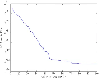
Figure 5.3 L2 Error of the POD procedure with 100 samples . . . 72
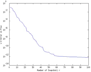
Figure 5.4 L2 Error of the POD procedure with 100 samples for the Adjoint Flux . . . 73
Figure 5.5 Effect of the Mesh Refinement on the POD-Error . . . 74
Figure 5.6 First Three POD-basis for the Forward Flux of the Fast Flux Part 75 Figure 5.7 First Three POD-basis for the Forward Flux of the Thermal Flux Part . . . 75
Figure 5.8 First Three POD-basis for the Adjoint Flux of the Fast Flux Part 76 Figure 5.9 First Three POD-basis for the Adjoint Flux of the Thermal Flux Part . . . 76
Figure 5.10 Worst Relative L2 Norm Error in Flux with Different POD Ap-proaches . . . 78
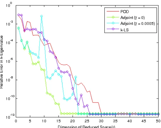
Figure 5.11 Worst Relative Error ink-Eigenvalue with Different POD Approaches 78 Figure 5.12 Relative L2 Norm Errors in Flux with the POD-basis (r= 15) . . 79
Figure 5.13 Relative L2 Norm Errors in Flux with the POD-basis (r= 30) . . 80
Figure 5.14 Relative Errors in k-Eigenvalue with the POD-basis (r = 15) . . . 80
Figure 5.17 20 Realizations of Cell-Averaged Fast Flux . . . 82
Figure 5.18 20 Realizations of Cell-Averaged Thermal Flux . . . 83
Figure 5.19 20 Realizations of Adjoint Part of Cell-Edge Current in Fast Energy Group . . . 84
Figure 5.20 20 Realizations of Adjoint Part of Cell-Edge Current in Thermal Energy Group . . . 84
Figure 5.21 20 Realizations of Adjoint Part of Cell-Averaged Fast Flux . . . . 85
Figure 5.22 20 Realizations of Adjoint Part of Cell-Averaged Thermal Flux . . 85
Figure 5.23 First Three POD-bases of Fast Current Part . . . 86
Figure 5.24 First Three POD-bases of Thermal Current Part . . . 87
Figure 5.25 First Three POD-bases of Fast Flux Part . . . 87
Figure 5.26 First Three POD-bases of Thermal Flux Part . . . 88
Figure 5.27 First Three POD-bases of Adjoint Solution of Fast Current . . . . 89
Figure 5.28 First Three POD-bases of Adjoint Solution of Thermal Current . 89 Figure 5.29 First Three POD-bases of Adjoint Solution of Fast Flux . . . 90
Figure 5.30 First Three POD-bases of Adjoint Solution of Thermal Flux . . . 90
Figure 5.31 POD-Error in Eq.(3.4) for the Forward Solution . . . 91
Figure 5.32 POD-Error in Eq.(3.4) for the Adjoint Solution . . . 91
Figure 5.33 Comparison of the POD-Based Methods by Eq.(5.5) . . . 93
Figure 5.34 Comparison of the POD-based Methods using Relative Error in k-Eigenvalue . . . 94
Figure 5.35 Comparison of the POD-based Methods by Relative Error in k -Eigenvalue atr = 100 . . . 94
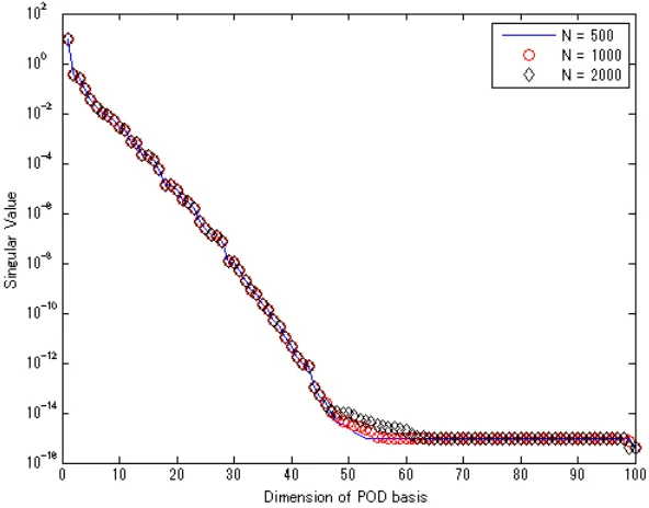
Figure 5.36 Comparison of the POD-based Methods using Eq.(5.5) at r= 50 . 95 Figure 5.37 Comparison of the POD-based Methods using Eq.(5.5) at r= 100 96 Figure 5.38 Comparison of the POD-Based Methods by Eq.(5.5) at r = 150 . 96 Figure 5.39 Singular Value Plot for Forward and Adjoint Solutions . . . 97
Figure 5.40 Comparison of POD-Based Method for the Scalar Flux . . . 98
Figure 5.41 Comparison of POD-Based Method for the k-Eigenvalue . . . 98
Figure 5.42 Comparison of POD-Based Method for the k-Eigenvalue atr = 50 99 Figure 5.43 Comparison of POD-Based Method for the k-Eigenvalue atr = 100 100 Figure 5.44 Comparison of POD-Based Method for the k-Eigenvalue atr = 150 100 Figure 5.45 Comparison of POD-Based Method for the k-Eigenvalue atr = 200 101 Figure 5.46 Comparison of POD-Based Method for the Flux at r= 50 . . . . 102
Figure 5.47 Comparison of POD-Based Method for the Flux at r= 100 . . . . 102
Figure 5.48 Comparison of POD-Based Method for the Flux at r= 150 . . . . 103
Figure 5.49 Comparison of POD-Based Method for the Flux at r= 200 . . . . 103
Figure 6.1 Condition Number of Legendre and Chebyshev Polynomials . . . 106
Figure 6.4 Comparison of Relative Error ink-eigenvalue with L1 andL2
Reg-ularization . . . 108 Figure 6.5 Comparison ofL1 Regularization with Different Number of Samples 109
Figure 6.6 Input Parameter Reduction of the Pin-Cell Model . . . 110 Figure 6.7 Coefficients of k-eigenvalue Interpolation recovered by OMP and
L2 Regularization . . . 112
Figure 6.8 Coefficients of 1st POD-basis,φ1j, recovered by OMP andL2
Reg-ularization . . . 113 Figure 6.9 Coefficients of 2nd POD-basis,φ2j, recovered by OMP andL2
Reg-ularization . . . 113 Figure 6.10 Coefficients of 3rd POD-basis, φ3j, recovered by OMP andL2
Reg-ularization . . . 114 Figure 6.11 Relative Error in k-Eigenvalue withL2 Regularization and OMP . 115
Figure 6.12 Relative L2 Error in Flux with L2 Regularization and OMP . . . 115
Figure 6.13 Error in Input Parameter Reduction . . . 117 Figure 6.14 Estimated Number of Samples Required to achieve desired accuracy
Chapter 1
Introduction
1.1
Background and Motivation
Nuclear reactor calculations are extremely complicated due to the complex nature of the physics of radiation interaction with matter as well as the heterogeneous nature
of reactor design, which often contains a great deal of spatial details. The complexity
of these models makes it difficult to execute the engineering-oriented analyses such as
sensitivity and uncertainty analysis, essential to assess the credibility of the simulation.
Any of these analyses require many executions of the model, often proportional to and
exponentially dependent on the number of input parameters. For typical reactor models,
the number of parameters can range from between hundreds to millions depending on the
level of details captured by the model. This renders uncertainty analysis computationally
intractable for reactor calculations. To overcome this problem, the scientific community
has focused on using reduced order modeling techniques to replace the original complex code with an inexpensive surrogate model that can be executed repeatedly for various
engineering analyses. There are a great number of methods developed over the years
for surrogate model construction, each with its own advantages and disadvantages. A
common theme to these methods is that the computational cost required to build the
surrogate is also dependent on the number of parameters, which makes its construction
difficult. Moreover, the accuracy of the surrogate is often difficult to quantify, which is
a pre-requisite for ensuring the results of all subsequent analyses using the surrogate are
credible. We focus in this thesis on a class of reduced order modeling techniques, referred
model are reduced by confining variations to a subspace, called active subspace. The
implication is that variations orthogonal to the active subspace are not significant and
can be ignored. If the size of the active subspace is small enough, huge reduction in the
computational cost for surrogate construction can be achieved. More importantly, using
recent developments, one can show that the errors resulting from the reduction can be
bounded to ensure credibility of the surrogate predictions.
Subspace Approach as Reduced Order Modeling
Historically, engineering applications of reduced order modeling techniques have
gained popularity in the hydraulics community because of the high computational cost
of the models under consideration, but reduced order modeling itself can be traced back
to the mathematics of interpolation, truncated Taylor expansion, Method of Weighted Residuals and so on. Reduced order modeling are be defined as a process by which
solu-tions to complex models can be described using few degrees of freedom, smaller than the
dimension of the complex solution. For example, assuming the model solution is described
by a function in one dimension evaluated atN points as determined by the discretization technique used to obtain the numerical solution. If one can approximate this function by
a number of select functions, say r which is less than N, then one has a reduced order model. This follows as now the function depends on r degrees of freedom rather than
N. One may argue that any engineering model can be considered a reduced order model of the exact model (often unknown). This follows since the physical phenomenon under consideration often has large degrees of freedom than engineering models. ROM
tech-niques can be distinguished based on the type of functions employed for the expansion.
Once an appropriate selection is made, one can re-cast the original model into one with
much fewer equations, which can be readily solved more efficiently. The choice of the
ex-pansion functions is fundamental to the success of this reduction approach. This choice
is expected to depend on the model, and therefore expert judgment is often needed to
make an educated choice. Moreover, calculating the errors resulting from this reduction
is an important step of the analysis. This error can be estimated a posteriori, i.e., after
the reduced model is constructed, by comparing its predictions to the original models. Important examples of such approaches are the spectral expansion method and the
method of weighted residuals [2, 3]. In both methods, a set of orthogonal functions can
of the expansion when the solution is sufficiently smooth [2].
The most common engineering approaches for reduced order modeling are the Proper
Orthogonal Decomposition Galerkin projection approach [4, 5]. The Proper Orthogonal
Decomposition is one of the common subspace approaches found in engineering
disci-plines. In the subspace approach, the structure of the solution to the system of stochastic
PDEs is represented by the linear combination of minimum number of the orthogonal
ba-sis functions or vectors. In this method, the original system of PDEs is projected onto the
reduced order subspace generated by the proper orthogonal decomposition. This method
is extensively applied in fluid dynamics community. One common example is a linear matrix equation of the form:
Ax=b (1.1)
and some results are demonstrated [4, 5].
The
k
-Eigenvalue Problem in Neutronics
In neutronics problems, most problems can be categorized into two major matrix
forms:
1) Source-driven problem:
Lφ=qsource. (1.2)
2) Generalized eigenvalue problem:
Lφ= 1
kFφ. (1.3)
In the source-driven problem, Eq.(1.2), the structure of the problem is the same as
Eq.(1.1) and the Proper Orthogonal Decomposition Galerkin projection approach can be
easily applied. However, in the case of the generalized eigenvalue problem, the method is
not directly applicable. Historically in nuclear engineering community, generalized eigen-value problem has been solved by the power iterative method and its variants which
are summarized in the following algorithm??. In this thesis we propose two approaches
to extend the applicability of POD techniques to generalized eigenvalue problems, one
Algorithm 1 Pseudo Algorithm for Power Iterative Method [6]
Set k0 =kinitial
Set the initial guess, φ0 =φinitial s= 0
while ||φ(s)−φ(s−1)||>
φ,1(1−ρ (s)
φ ) or ||k(s)−k(
s−1)||>
k(1−ρ
(s)
k )do s=s+ 1
Calculate qsource(s) = k(s1−1)Fφ
(s−1)
Solve Lφ(s) =qsource(s) .
Update k-eigenvalue, k(s) =k(s−1) RdV νfΣfφ(s)
R
VdV νfΣfφ(s−1)
Approximate the spectral radius of φ(s), ρφ(s) = ||φ||φ(s(−s)1)−φ−φ(s(−s−1)2)||∞||
∞
Approximate the spectral radius of k(s), ρk(s)= ||k||k(s(−s)1)−k−k(s(−s−1)2)||∞||
∞
end while
One can easily show that Lφ(s) = q(sources) can be solved by the Proper Orthogonal
Algorithm 2Pseudo Algorithm for Power Iterative Method with POD-Galerkin Method Denote that a reduced order transform operator as Uthat is an orthogonal matrix
Set k0 =kinitial
Set the initial guess, φ0 =φinitial s= 0
Project the matrix operator L onto the reduced order subspace ˜L=UTLU while ||φ(s)−φ(s−1)||> φ,1(1−ρ
(s)
φ ) or ||k
(s)−k(s−1)||>
k(1−ρ
(s)
k )do s=s+ 1
Calculate qsource(s) = k(s1−1)Fφ
(s−1)
Project the source term onto the reduced order subspace, ˜qsource(s) =UTq(sources)
Solve ˜Lφ˜(s) = ˜q(s)
source.
Project back onto the original space, φ(s) =UTφ˜(s)
Update k-eigenvalue, k(s) =k(s−1) RdV νfΣfφ(s)
R
VdV νfΣfφ(s−1)
Approximate the spectral radius of φ(s), ρ(s)
φ =
||φ(s)−φ(s−1)||∞
||φ(s−1)−φ(s−2)||∞
Approximate the spectral radius of k(s), ρ(s)
k =
||k(s)−k(s−1)||∞
||k(s−1)−k(s−2)||∞
end while
This approach is very efficient and one can expect to achieve large reduction in
com-putational cost and time. In addition, it is important to note that this method can be
applied to the other acceleration techniques commonly applied in Nuclear Engineering.
For example, the shifted-inverse power iterative method can be modified with the
Algorithm 3 Pseudo Algorithm for Shifted-Inverse Power Iterative Method with POD-Galerkin Method adapted from [7]
Denote that a reduced order transform operator as U
Set a scalarσ that is close to 1/k
Set k0 =kinitial
Set the initial guess, φ0 =φinitial s= 0
Project the matrix operator L onto the reduced order subspace ˜L=UTLU while ||φ(s)−φ(s−1)||>
φ,1(1−ρ (s)
φ ) or ||k(s)−k(
s−1)||>
k(1−ρ
(s)
k )do s=s+ 1
Calculate qsource(s) = k(s1−1)Fφ
(s−1)
Project the source term onto the reduced order subspace, ˜qsource(s) =UTq(sources)
Solve ( ˜L−σI) ˜φ(s) = ˜qsource(s) .
Project back onto the original space, φ(s) =UTφ˜(s)
Update k-eigenvalue, k(s) =k(s−1)
R
dV νfΣfφ(s)
R
VdV νfΣfφ(s−1)
Approximate the spectral radius of φ(s), ρφ(s) = ||φ||φ(s(−s)1)−φ−φ(s(−s−1)2)||∞||
∞
Approximate the spectral radius of k(s), ρk(s)= ||k||k(s(−s)1)−k−k(s(−s−1)2)||∞||
∞
end while
The algorithm is almost same with the power iterative method. However, the rate of
convergence is dramatically improved if σ≈1/k and the rate of convergence is given by [7]
d= |1/k1−σ|
|1/k2−σ|
(1.4)
where k1 is the dominant eigenvalue and k2 is the second dominant eigenvalue. One
can also apply the Rayleigh Quotient Iteration since forming the explicit inverse is not
expensive in the reduced space. However, these approaches require extra dense
matrix-vector multiplications in each iterative step. In addition, modern fast iterative solvers
1.2
Thesis Contents
This thesis develops hybrid reduced order modeling methods to generate surrogates
for models described as generalized eigenvalue problems. Chapter 2 briefly describes the
neutronics model employed and chapter 3 describes the mathematical framework of ROM
methods. Chapter 4 briefly presents theory of the generalized polynomial chaos, sparse
approximation and input parameter reduction. Numerical experiments are documented
Chapter 2
Neutronics Problem
In reactor simulation, the determination of the multiplication factor, k, and the distribution of neutrons in space and energy is the fundamental task for reactor
engi-neers because this knowledge helps one sustain and control the fission chain reaction.
In reactor physics, two major approaches to determine these quantities are the diffusion
approximation and the transport approximations. Neutrons are treated as a diffusive material like gas molecules in the diffusion approximation. In the transport
approxima-tions, the distribution of neutrons is described by the Boltzmann equation which is an
integro-differential equation, and is much more difficult to solve than diffusion equation.
The diffusion approximation can be derived from the transport equation under some
simplifying assumptions.
2.1
The Diffusion Approximation
The basics of neutron diffusion theory are well presented in the textbooks from Duder-stadt and Hamilton [8] and Stacey [9]. The neutron diffusion equation can be written
as:
∇J(r, E) + Σt(r, E)φ(r, E) =
Z ∞
0
dE0Σs(r, E0 →E)φ(r, E0)
+χ(E)
k
Z ∞
0
with Fick’s law giving:
J(r, E) =−D(r, E)∇φ(r, E) (2.2)
wherer is the position vector, E is the neutron energy, J is the neutron current, φ(r, E) is the scalar neutron flux, Σ(r, E) is the total macroscopic cross-section, Σs(r, E0 →E) is
the macroscopic scattering cross-section,χ(E) is the fission yield spectrum, ν(E0) is the average number of neutrons born in a fission, Σf(r, E) is the macroscopic fission
cross-section, andD(r, E) is the diffusion coefficients. To solve this equation, one can discretize the equation directly or combine Eq.(2.1) and Eq.(2.2) to obtain the P0 equation.
In the former case, the neutron energyE is divided intoGenergy groups and Eq.(2.5) is integrated over each energy group. That can be written as:
∇Jg + Σgtφg = G
X
g0=1
Σgs0→gφg0 +
χg k
G
X
g0=1
νgΣg
0
fφg0, g= 1,· · ·G (2.3)
Jg =−Dg∇φg, g= 1,· · ·G (2.4)
where Eq.(2.3) can be spatially discretized by the finite element or finite difference method
with appropriate boundary conditions. For the latter case, Eq.(2.1) and Eq.(2.2) are combined into the P0 equation:
− ∇ ·D(r, E)∇φ(r, E) + Σt(r, E)φ(r, E) =
Z ∞
0
dE0Σs(r, E0 →E)φ(r, E0)
+χ(E)
k
Z ∞
0
dE0ν(r, E0)Σf(r, E0)φ(r, E0) (2.5)
then Eq.(2.5) is discretized into the multi-group neutron diffusion equation:
− ∇ ·Dg∇φg+ Σ g tφg =
G
X
g0=1
Σgs0→gφg0 +
χg k
G
X
g0=1
νgΣ g0
fφg0, g= 1,· · ·G (2.6)
which can be solved by the finite element method or finite difference method. For the
finite difference method, see Stacey [9] and Duderstadt and Hamilton [8] for examples.
The k-eigenvalue diffusion equation can be written in block matrix form. For the P0
equation, it is given by:
φ =hφT
1 · · · φTi · · · φTG
iT
where φi is a vector of discretized scalar flux in energy group. Then, Eq.(2.6) can be
rewritten in sparse block matrix form:
Lφ=λFφ (2.8)
where L=
∇+Σ1R −Σs2→1 · · · −ΣG→s 1
−Σ1s→2 ∇+Σ2R · · · −ΣG→2
..
. ... . .. ...
−Σ1s→G −Σ2s→G · · · ∇+ΣGR
(2.9) F=
χ1ν1Σ1f χ1ν2Σ2f · · · χ1νGΣGf χ2ν1Σ1f χ2ν2Σ2f · · · χ2νGΣGf
..
. ... . .. ...
χGν1Σ1f χGν2Σ2f · · · χGνGΣGf
(2.10)
where ∇ is a matrix resulted from the discretization of the ∇ operator on the scalar flux φi and ΣgR is a diagonal matrix defined as the group removal cross-section to be
ΣgR=Σgt−Σg→gs resulting from the discretization. The P1equation can also be discretized
in a similar manner.
2.2
Newton’s Method for k-Eigenvalue Problem
Finding the fundamental eigenpair (eigenvalue and eigenvector) is the computational
burden for large scale problem. Historically in nuclear engineering, this generalized eigen-value problem is solved by the power iterative method, but the rate of convergence is
slow for models with the dominance ratio very close to 1.0 [10]. Over the past three
decades, a variety of approaches has been proposed to accelerate the convergence of the
solution, eg. Wielandt shift approach [11] and Chebyshev acceleration [12]. Recently, the
Newton-Krylov approach is beging considered for multi-group neutronics calculations
[13]. Newton’s method is characterized by its quadratic convergence and difficulty in
calculating and inverting a Jacobian matrix to obtain the Newton step.
As shown in the previous section, the multi-group diffusion problem can be written
in a generalized eigenvalue form:
and assume a constraint on the eigenpair denoted by:
f(λ, φ) = 0. (2.12)
Note that it is common to usef(λ, φ) = φTφ−1, so this constraint is used in this section. Then, finding eigenpairs is equivalent to minimizing a residual function defined by:
R(λ, φ) =
"
Lφ−λFφ f(λ, φ)
#
. (2.13)
Whenλandφare eigenpairs, the residual function is equal to zero. This is also considered as an optimization problem, which can be solved by Newton’s method. To find a solution,
expand Eq.(2.13) around the initial guess λ0 and φ0:
R(λ, φ) = R(λ0, φ0) +J(λ0, φ0)
"
∆λ
∆φ
#
+· · · (2.14)
where ∆λ =λ−λ0, ∆φ=φ−φ0 and the Jacobian matrix is given by [13]:
J(λ, φ) =
"
L−λ0F −Fφ0
2φT
0 0
#
(2.15)
Now, setting R(λ, φ) = 0, the equation for the Newton step is given by:
−R(λ0, φ0) =J(∆λ,∆φ)
"
∆φ0
∆λ0
#
(2.16)
Therefore, each Newton step is given by:
"
∆φi+1
∆λi+1
#
=J−1(λi, φi)R(λi, φi) (2.17)
It is important to note that the exact Newton’s method is computationally prohibitive to
calculate. Therefore, the inverse of the Jacobian matrix is calculated by iterative methods such as the Krylov subspace method or a fixed-point iteration. The efficiency of Krylov
subspace method is governed by a preconditioner and incomplete LU factorization is
precon-ditioners efficiently. Otherwise, the incomplete factorization takes long time and number
of non-zero elements in preconditioners is extremely large to store. The study on the
Newton’s method in Nuclear Engineering application is a quite recent topic (See [14] for
the details).
2.3
Transport Calculation by T-NEWT sequence
The neutron transport equation is more accurate compared with the diffusion
approxi-mation. The general form of the neutron transport equation is given as:
ˆ
Ω·∇~ψ(r,Ωˆ, E) + Σt(~r, E)ψ(~r,Ωˆ, E) =Q(~r,Ωˆ, E) (2.18)
where ψ(~r,Ωˆ, E) angular flux, Σt total cross-section, and Q(~r,Ωˆ, E) source term. The
source term Qis composed of three components: 1. a scattering source:
S(~r,Ωˆ, E) =
Z
4π dΩˆ0
Z
4π
dE0Σs(~r,Ωˆ0 →Ωˆ, E0 →E)ψ(~r,Ωˆ0, E0) (2.19)
2. a fission source:
F(~r,Ωˆ, E) = χ(~r, E) 4π
Z ∞
0
dE0νf(~r, E0)Σf(~r, E0)φ(~r, E0) (2.20)
and 3. an external source or fixed source:Sext(~r, E). To formulate the k-eigenvalue
prob-lem, recast Eq.(2.18) into an equation of the form:
ˆ
Ω·∇~ψ(r,Ωˆ, E) + Σt(~r, E)ψ(~r,Ωˆ, E) =
Z
4π dΩˆ0
Z
4π
dE0Σs(~r,Ωˆ0 →Ωˆ, E0 →E)ψ(~r,Ωˆ0, E0)
+χ(~r, E) 4πk
Z ∞
0
dE0νf(~r, E0)Σf(~r, E0)φ(~r, E0) (2.21)
T-NEWT is TRITON sequence to solve 2D transport equation by NEWT in SCALE
developed by Oak Ridge National Laboratory. NEWT is a 2D multi-group
discrete-ordinates radiation transport code with complex geometry developed by Oak Ridge
for T-NEWT sequence can be found in the appendix.
2.4
Model Description
For uncertainty quantification, five different neutronics problems are considered. Each
model is assumed to have uncertainties in cross-section data or atomic density values.
Each model has a different number of stochastic variables.
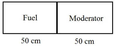
A. 1D Simple Fuel Model
Case A is a simple two-group neutron diffusion equation that consists of uranium (left)
and water (right) with equal widths ofw= 50 cm. The two-group diffusion equation for this model is given by
−D1(x, ξ)
∂2
∂x2φ1(x, ξ) + Σ 1
R(x, ξ)φ1(x, ξ)
= 1
kχ1(x, ξ)ν1(x, ξ)Σ
1
f(x, ξ)φ1(x, ξ) +
1
kχ1(x, ξ)ν2(x, ξ)Σ
2
f(x, ξ)φ2(x, ξ)
−D2(x, ξ)
∂2
∂x2φ2(x, ξ) + Σ 2
R(x, ξ)φ2(x, ξ)−Σs1→2(x, ξ)φ1(x, ξ) = 0
where the induced neutrons are assumed to be born only in the energy group 1. Fig. 2.1
shows the geometry of this simple fuel model. A Neumann boundary condition is assigned
to the left boundary whereas a Dirichlet boundary condition is assigned to the right
boundary.
The boundary conditions are described as:
d dxφg
x=0
= 0
φg|x=2w = 0
In addition, a constraint is imposed on the fluxes:
2
X
g=1
φTgφg = 1
Then, this model is discretized into generalized eigenvalue problem of the form:
Lφ = 1
kFφ
where φ = hφT
1 φT2
iT
where φi is a vector of discretized flux of the energy group i.
Table 2.1 shows the cross-section data for this model. To simulate uncertainty in this
model, the cross-section data are assumed to have uncertainty in the values.
Table 2.1: Test Model A Cross-Section Data [8]
Fuel Moderator
1 of 2 2 of 2 1 of 2 2 of 2
νΣf .008476 .18514 0.0 0.0
Σa 0.01207 0.1210 0.0004 0.0197
D 1.2627 .3543 1.13 0.16
ΣR 0.02619 0.1210 0.0494 0.0197
The thermal group absorption cross-section and the removal cross-section are assumed
to be equal, and hence the total number of stochastic variables is 12. The model is
spatially discretized with equal node width resulting in 1000 total nodes, and hence the
dimension of L and F is 2000 (because the number of unknowns per node is equal to two,
representing the two-group flux).
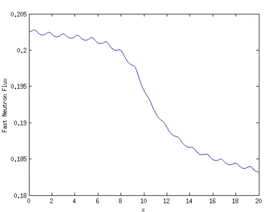
group neutron flux distribution with the reference cross-section values.
Figure 2.2: Fast Group Flux Distribution
B. 1D Assembly Model
The test model B is a two-group neutron diffusion model describing a 1-D fuel assembly
model consisting of MOX and UO2 with reflective boundary conditions at both sides [15].
The width of each assembly is 10 cm and consists of 8 fuel pins surrounded on both sides
by water that are spatially discretized with equal node width. Fig. 2.4 and Fig. 2.5 show
the geometry of this model.
Figure 2.4: The Geometry of Assembly
Figure 2.5: The Geometry of Pin Cell
The form of the neutron diffusion equation for this model is given by:
d dxJ
g(x, ξ) + Σg
R(x, ξ)φg(x, ξ) =
2
X
g0=1,g06=g
Σgs0s→g(x, ξ)φg0(x, ξ) +
χg(x, ξ) k
2
X
g0=1
with Fick’s law giving an expression for the neutron current:
Jg(x, ξ) =−Dg(x, ξ) d
dxφg(x, ξ)
Then, discretize the assembly into I equal width cells where each cell is defined for
x∈[xi, xi+1] and the value of the cell edge locations is given by:
xi = L
I(i−1)
Then, this diffusion equation can be discretized using the cell-edge current Jg,i, the
cell-edge flux φg,i, and the cell-average flux ¯φg,i:
Jg,i+1−Jg,i+ Σ g
Rφ¯g,ih−
2
X
g0=1,g06=q
Σgs0→gφ¯g,ih = χg
k
2
X
g0=1
νfg0Σgf0φ¯g,ih Dg,i(φg,i+1−φ¯g,i) +
1
2Jg,i+1h = 0
Dg,i(φg,i−φ¯g,i) +
1
2Jg,ih = 0 ¯
φg,1−φg,1 = 0
φg,I+1−φ¯g,I = 0
where h=xi+1−xi and the cell-average flux is defined as:
¯
φg,i =
Z xi+1 xi
φg(x)dx
Then, the model is simplified into generalized eigenvalue problem of the form:
Lx= 1
kFx
where x =hJT
1 J2T φT1 φ2T φ¯T1 φ¯T2
iT
which represent the discretized quantities.
Ta-ble 2.2 shows the cross-section data for this model. The cross-section data are assumed
Table 2.2: Test Model B Cross-Section Data [15]. Σf1, νf1, ¯µ10, Σs2→1, χ1, ¯µ20 are all zero. Cross-Sections Σ1
t Σ1 →1
s Σ1 →2
s χ1 Σ2t Σ2 →1
s Σ2f νf2
MOX fuel 0.2 0.185 0.015 1 1.2 0.9 0.3 1.5
Uranium fuel 0.2 0.185 0.015 1 1.0 0.9 0.1 1.5
Water 0.2 0.17 0.03 0 1.1 1.1 0 0
with a normalization constraint
h
2
X
g=1
¯
φTgφ¯g = 1
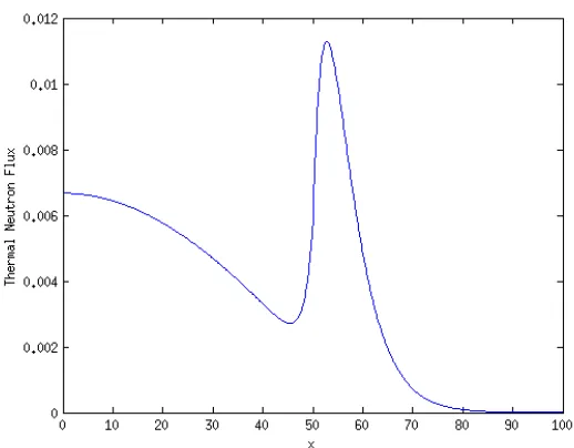
Figure 2.7: Thermal Group Flux Distribution
Fig. 2.6 and Fig. 2.7 show the fast and thermal neutron flux distribution for the
reference cross-section values.
C. 2D MOX Fuel Calculation
The test model C is a 2D transport model describing a fresh MOX fuel from the Phase
IV-A Burn-up Credit Benchmark by OECD/NEA Burn-up Credit Working Group [16].
The geometry for this model is an infinite PWR fuel cell lattice as shown in Fig. 2.8. The Fuel pin pitch is 1.33 cm square pin array, the fuel pellet radius is 0.412 cm and the
cladding thickness is 0.0063 cm. In this model, it is assumed that no air or helium gas is
Figure 2.8: Geometry of MOX fuel pin cell for PWR
In reference [16], three different types of MOX fuels are considered. However, only the case A, a typical plutonium composition for material derived from the reprocessing
of thermal reactor UO2 fuel, is considered. Table 2.3-Table 2.4 show the material
com-positions for Case A. These models are evaluated using the SCALE code package with
END/F V 44 energy group cross-section data with CENTRAM. Appendix A shows the
input file for the T-NEWT sequence. In the original benchmark problem, the discrete
ordinates calculations were performed usingS8 quadrature andP3 scattering for all
mix-ture. However, in uncertainty quantification, many model evaluations are necessary and
the calculation is reduced by simplying scattering order to 2 in all moderator materials
Table 2.3: Non-fission material compositions [16]
Nuclide Atoms/Barn.cm
Zr 4.2982E-2
Fe 1.4838E-4
Cr 7.5891E-5
H 6.6724E-2
O 3.3362E-2
Table 2.4: Material Compositions for Fresh MOX Case A [16]
Nuclide Atoms/Barn.cm Nuclide Atoms/Barn.cm
234U 2.7999E-7 235U 1.4838E-4
238U 2.3074E-2 238Pu 2.4700E-5
239Pu 8.0623E-4 240Pu 3.1298E-4
241Pu 1.6533E-5 242Pu 5.3981E-5
16O 4.8992E-2
D. 2D Quarter Assembly Calculation
The test model D is 2D 8×8 quarter assembly model. Appendix A shows the sample input
file for this model. This problem can be found in the SCALE sample problem directory.
However, the fuel composition is modified into MOX fuel as described in the test case C.
Fig. 2.9 shows the geometry of the quarter assembly models.
Fig. 2.10-2.11 show the selected output from the test problem D. Detailed material
composition and geometric information can be found in the sample input in Appendix
Figure 2.9: Geometry of Quarter Assembly Model
Figure 2.11: Group 44 Flux
E. 2D Pin-Cell Model by Diffusion Approximation
The last model to be considered is a pin-cell model using the 44 group finite element
diffusion equation. The geometry for this model is an infinite PWR fuel cell lattice as
shown in Fig. 2.12. The Fuel pin pitch is 1.3127 cm square pin array, the fuel pellet radius
is 0.410 cm and the cladding thickness is 0.0065 cm. No air/helium gap is assumed in
these models. Different from model C, the MOX fuel is irradiated with 40GWd/teHM
followed by one year of cooling in water. Table 2.5 shows the reference values of the
materials of this model. Each atomic density is assumed to have uncertainty in its value
Table 2.5: Material Compositions for MOX Case A (40GWd/teHM) with one year cool-ing
Nuclide Atoms/Barn.cm Nuclide Atoms/Barn.cm
234U 7.7718E-7 235U 2.9018E-5
236U 6.1753E-6 238U 2.2365E-2
238Pu 2.5504E-5 239Pu 4.5028E-4
240Pu 2.9067E-4 241Pu 1.8125E-4
242Pu 9.1733E-5 237Np 3.0746E-6
241Am 2.4023E-5 243Am 2.4023E-5
16O 4.8992E-2 242Cm 6.7186E-7
243Cm 6.7186E-7 244Cm 1.3749E-5
245Cm 1.6967E-6 95Mo 4.4441E-5
99Tc 5.3736E-5 101Ru 5.774E-5
103Rh 4.9708E-5 109Ag 1.1408E-5
133Cs 5.7100E-5 143Nd 3.8610E-5
145Nd 2.8038E-5 147Sm 5.2265E-6
149Sm 3.3504E-7 150Sm 1.3820E-5
151Sm 1.5043E-6 152Sm 6.2143E-6
153Eu 7.5074E-6 155Gd 1.4403E-7
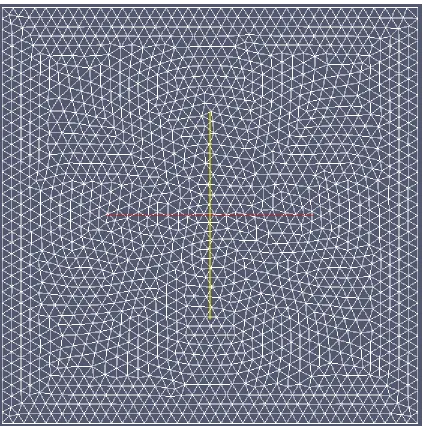
Fig. 2.12 shows the triDelaunay mesh used for this model. The number of elements
in this triDelaunay mesh is 1703. Therefore, the dimension of L and F is 74932. The
number of non-zero elements is L is 12869931 and that of F is 71206081. Fig. 2.13-2.14
show sparsity patterns ofLandF. Fig. 2.15-2.16 show the sparsity of the reorderedLand
F. It is obvious that Land F are highly sparse and reorder L andF saves large amount of time in incomplete factorization. Fig. 2.17-2.18 show the selected fluxes calculated by
the reference value. Using MATLAB, this large problem can be solved within 40 seconds
using the reverse symmetric Cuthill-Mckee reordering with GMRES.
Figure 2.13: Sparsity ofL
Figure 2.15: Sparsity of reordered L
Figure 2.17: 12th Energy Group Flux
Chapter 3
Subspace Method for Reduced
Order Modeling
The computational cost of the simulation of the nuclear reactor system has
signifi-cantly increased over the past few decades as accuracy requirements have become much more stringent to gain both regulatory and public acceptance. There are currently several
initiatives around the country aiming to develop advanced codes for reactor simulation.
These codes are expected to be high dimensional and expensive to run. This implies that
surrogate model techniques must be improved to allow one execute engineering
applica-tions such as uncertainty quantification in a practical manner.
In regard to the neutronics problem, the k-eigenvalue problem is the most expen-sive part of the analysis. Classically, finding the fundamental eigenpair (eigenvector and
eigenvalue) is done by the power iterative method which converges slowly for the models
associated with the dominance ratio very close to 1.0 [10]. Over the past three decades, a variety of approaches have been proposed to accelerate the convergence of the solution
such as the Wielandt shift approach [11] and Chebyshev acceleration [12]. However, as
the engineering model becomes more detailed, the computational requirements increase
at quadratic rate for memory and cubic rate for computations for the dense matrix. This
makes the execution of the high fidelity models computationally prohibitive unless one
has access to High Performance Computing facilities.
To overcome the challenge, reduced order modeling (ROM) techniques have been
promoted over the past few decades. It is important to note that ROM is referred to
Prin-cipal Component Analysis, Snapshot Method, model order reduction and row-rank
ap-proximation are all examples of ROM techniques. The objective of the ROM techniques
is to reduce the computational burden without losing the accuracy of original models
with a known error bound if possible. In ROM, the dimension of the original model is
re-duced to a low-dimensional problem that can be executed with lower computational cost.
With this reduction, the reduced problem can be executed many times for uncertainty
quantification and sensitivity analysis.
Two basic approaches have been applied for surrogate model construction. One of
them is a spectral approach and the other is the input parameter reduction. In the
former approach, the response is expressed as a linear combination of arbitrary orthogonal basis functions, e.g., trigonometric functions and Legendre polynomials. The generalized
Polynomial Chaos (gPC) expansion is considered to be a spectral method. Note that
many functions other than orthogonal basis functions can also be used. For example,
the sparse grid approximation expands the response as a linear combination of hierarchy
hat basis functions.[17]. The spectral approach has the desirable property that the error
decays at the exponential rate [2].
In the second approach, the effective number of input parameters is reduced by the
finding an active subspace in the input parameter space. This is possible because for
many realistic models the response depends on a few degrees of freedom (DOF), where each degree of freedom represents a function of all the parameters combined. If linear
functions are employed to describe the relationship between the active DOFs and original
input parameters, the ROM problem reduces to a linear algebra problem, where the
active DOFs are described by a subspace. The implication is that parameter variations
orthogonal to this subspace will produce negligible variations in the response subspace
[18, 19].
In this chapter, recently developed and well-established approaches for ROM are
briefly reviewed. In addition, ROM techniques for the generalized eigenvalue problem are
3.1
Method of Snapshot
In chapter 2, the multi-group neutron diffusion equation is expressed as a generalized
eigenvalue problem of the form Lφ = λFφ. Now, assume that the multi-group neutron diffusion equation has uncertainties in cross-section values and atomic densities. Then,
represent the uncertainties by a stochastic variable vectorξ where ξ iss×1 ands is the number of uncertain parameters. Now, insertξ into a generalized eigenvalue problem,
L(ξ)φ(ξ) = λ(ξ)F(ξ)φ(ξ) (3.1)
which is the stochastic generalized eigenvalue problem (SGEP) discretized from SPDE
and further assume that the dimension ofφ(ξ) isn×1. For the high fidelity model, solving the SGEP multiple times is computationally expensive and a surrogate model with high
accuracy is required. This can be achieved by employing Proper Orthogonal
Decomposi-tion (POD) to obtain an optimal low dimensional basis to transform the high dimensional problem into the low dimensional one: see [4, 5] for a more detailed introduction. In other
words, the goal is to represent the solution to SGEP using a POD-basis:
φ(ξ)≈
r
X
i=1
αi(ξ)Φi (3.2)
where Φiare the POD basis,αi(ξ) are undetermined coefficients, andris the dimension of
the POD basisdesired to be as small as possible. In addition, another important objective of the POD-based method is to find the error bound of the form:
φ(ξ)− r X i=1
αi(ξ)Φi
≤ (3.3)
where is an upper bound of the errorwhere the undetermined coefficients, α(ξ), are determined via a minimization problem. Unfortunately, the error bound for this form is
not known for the discrete case. Instead, it is common to use the following expansion:
m X j=1
φ(ξj)−
r
X
i=1
αi(ξj)Φi
2 X
where X denotes the Hilbert space of the spatial variables and ξj denotes the j-th
ran-domly sampled stochastic variables. To determine Φ, multiple approaches are proposed:
the method of snapshot with 1. eigenvalue decomposition [21], 2. singular-value
decom-position (SVD) [22], and 3. the range-finding algorithm [23].
The method of snapshots [24] is the POD procedure to express a solution to the SGEP
by a linear combination of snapshots φ(ξi) denoted by:
φ(ξ)≈
m
X
j=1
βj(ξ)φ(ξj) (3.5)
whereβi(ξ) are undetermined coefficients. In other words, a solution to SGEP is spanned by snapshots described as:
φ(ξ)∈span(φ(ξ1),· · · , φ(ξi),· · · , φ(ξm)). (3.6)
If Φ(ξj) = φ(ξj) in Eq.(3.4) and r = m, then Eq.(3.4) has = 0. However, the primary objective is to find Φi with r << n while minimizing .
3.1.1
Eigenvalue Decomposition
Eigenvalue decomposition is one possible method to accomplish this goal. Assume a
matrix Y whose columns are known snapshots of the form:
Y =
h
φ(ξ1) · · · φ(ξm)
i
(3.7)
where the dimension Y isn×m. Now, the expression in this form becomes:
YTYxi =µixi (3.8)
wherexiandµiare thei-th eigenpair for the symmetric matrixYTY. SinceYTYis a
real-symmetric matrix,µi are always non-negative. Without loss of generality, the eigenvalues µi are assumed to be descending order, µ1 ≥ · · · ≥µm. The method of snapshots shows
that an optimal error can be obtained by the POD-basis expressed as [21]:
Φi =
1
√
µi
and the optimal error bound for Eq.(3.4) is given by [21]: 1 m m X j=1
φ(ξj)−
r
X
i=1
hΦi, φ(ξj)iΦi
2 X = m X
i=r+1
µi (3.10)
where h,iis the inner product defined as:
ha, bi=aTb. (3.11)
3.1.2
Singular Value Decomposition
The same error bound can be obtained by the singular value decomposition (SVD). The
error bound for SVD is derived using the error bound by the eigenvalue decomposition
using the relation between the singular values and eigenvalues. More formal derivation
for the error bound of Eq.(3.4) with the singular value decomposition can be found in
[22].
SVD is one of the most important tools in numerical linear algebra due to its broad
applications in theory and engineering. The SVD is defined as the following manner: Let A∈Cm×n. Then reduced SVD of A is given by:
A=UΣV∗ (3.12)
where Σ= σ1 . .. σn (3.13)
with σ1 ≥ · · · ≥ σmin(m,n) ≥0 and with U∈Cm×m and V ∈Cn×n are unitary. Now, the
error bound for Eq.(3.4) can be obtained using this definition.
Assume an eigenvalue decomposition for Y∗Y implying Y∗Yxi = µixi and SVD
for Y, Y = UΣV∗. Then, one can obtain the relation between singular values and eigenvalues:
µi =σ2i. (3.14)
eigenvalue decomposition of the form:
Y∗Y =XMX∗ (3.15)
where X is an orthogonal matrix and M is a real diagonal matrix with the eigenvalues
of Y on the diagonal. Likewise, using SVD, Y∗Y can be factored as:
Y∗Y = (UΣV∗)∗UΣV∗ =VΣ2V∗ (3.16)
Since V is unitary and Σ2 is a real diagonal matrix, implying that Σ2 =M. Hence,
µi =σi2
and V =X. Now, Eq.(3.10) can be written using SVD. SinceV =X, it is obvious that
xi =vi. Now, Eq.(3.9) can be written by the singular value and left singular vector:
Φi =
1
√
µi
Yxi =
1
σi
Yvi =
1
σi
UΣV∗vi =ui (3.17)
Then, Eq.(3.10) is written as:
1 m
φ(ξj)−
r
X
i=1
hΦi, φ(ξj)iΦi
2 X = m X
j=r+1
µi = m
X
j=r+1
σ2j (3.18)
Therefore, Eq.(3.18) gives an equivalent error bound for SVD. Regardless of whether we
choose SVD or eigenvalue decomposition, both forms have the same error bound.
However, the error bound given by Eq.(3.4) is inconvenient in some cases. Therefore,
we propose a slightly different error bound:
φ(ξj)−
r
X
i=1
hΦi, φ(ξj)iΦi
2
≤ for ∀j (3.19)
The optimal solution to Eq.(3.19) is not known, but the upper bound can be obtained
with SVD given by:
φ(ξj)−
r
X
i=1
hΦi, φ(ξj)iΦi
2
Proof. Assume an SVD ofY,Y =UΣV∗ whereU∈Rm×m,Σ∈
Rm×n, and V∈Rn×n. Then, Eq.(3.19) is written as:
φ(ξj)−
r
X
i=1
hΦi, φ(ξj)iΦi
2 =
φ(ξj)−UrU∗rφ(ξj)
2 (3.21)
where Ur represents the first r columns of Udenoted as:
Ur=
h
u1 u2 · · · ur
i
(3.22)
and Un−r as:
Un−r =
h
ur+1 ur+2 · · · um
i
(3.23)
and we have the identity:
I=UrU∗r+Un−rU∗n−r (3.24)
since I = UU∗ = hUr 0
i
+h0 Un−r
i h
Ur 0
i
+h0 Un−r
i∗
. Then, Eq.(3.21)
can be written in terms of the singular matrices:
φ(ξj)−
r
X
i=1
hΦi, φ(ξj)iΦi
2 =
φ(ξj)−UrU∗rφ(ξj) 2 =
UΣv∗j −UrU∗rUΣvj∗ 2 =
Un−rU∗n−rUΣvj
2
≤ ||Un−r||2||Σn−r||2
vj∗
2
≤σr+1 (3.25)
since ||Un−r||2 = 1 and
v∗j
2 = 1.
3.1.3
Range Finding Algorithm
Another way to generate a basis for POD is the range-finding algorithm proposed in [23].
In the range-finding algorithm, instead of Eq.(3.5), the error is calculated according to:
This approach can be justified by considering Eq.(3.18). In Eq.(3.18), the POD-basis
is given by the dominant left singular vectors of Y. The left singular vectors form a
basis for the range of Y. Therefore, a good approximation of the range of Y will be a
good candidate for Q. If in Eq.(3.26) is small, then Q is a good approximation of the range of Y. The range-finding algorithm to calculate the POD basis is summarized in
Algorithm 4.
Algorithm 4 Range Finding Algorithm for the POD-Procedure [23]
Given an n×m matrix Y of snapshots, a tolerance , and an integer
k, the following algorithm computes a POD basis Q such that Eq.(3.26) holds with probability at least 1-min{m, n}10−k.
1. Draw standard Gaussian vectors ω(1),. . ., ω(k) of lengthn. 2. For i= 1,2,. . . , r, compute y(i) =Yω(i).
3. j = 0
4. Set Q= 0n×0
5. while max y(j+1)
, y(j+2)
,· · · , y(k+1)
≥/(10
p
2/π) (a) j =j+ 1
(b) Overwrite y(j) by (I−Q(j−1)(Q(j−1))∗)y(j)
(c) q(j) =y(j)/ y(j)
(d) Q(j) =Q(j−1) q(j)
(e) Draw a standard Gaussian vector ω(j+r) of length n.
(f) y(j+r) = (I−Q(j)Q(j)∗)Aω(j+r) for
Overwrite y(i) byy(i)−q(i)hq(i), y(i)i
end for
6. end while
Note that a better error bound for this form can be obtained using SVD given by:
min
Q ||(I−QQ
∗
)Y||=σi+1 (3.27)
where Q = Ui and Ui is a partitioned matrix of U = [Ui Um−i]. This is known as
the optimality of the singular value decomposition [25]. In other words, SVD is optimal
and more accuracy in the sense of Eq.(3.26). However, SVD would be computationally
more expansive than the range-finding algorithm. Therefore, the range-finding algorithm
is preferred for large scale problems.
3.1.4
Implementation of Method of Snapshots by
k
-Least Squares
Assume that a solution to the SGEP can be written as a linear combination of the
POD-basis given by:
φ(ξ)≈
r
X
i=1
α(ξ)Φi =Qα(ξ) (3.28)
whereQis the POD-basis andα(ξ) is the vector of undetermined coefficients. Then, plug Eq.(3.28) into the SGEP:
L(ξ)φ(ξ) = λ(ξ)F(ξ)φ(ξ)⇒L(ξ)Qα(ξ) =λ(ξ)L(ξ)Qα(ξ) (3.29)
where L and F are discretized matrices of dimension n×n and L(ξ)Q and F(ξ)Q are reduced matrices with dimensionn×r. Eq.(3.29) is called as overdetermined generalized eigenvalue problem. See [26] for its properties and how to solve this problem in general.
Since L(ξ)Q and F(ξ)Q are no longer square, traditional approaches such as the power iterative method and Krylov-type subspace methods are not applicable to this
prob-lem. Therefore, Eq.(3.29) is transformed to an optimization problem to find a desired
eigenpair. As discussed in Chapter 2, define a residual objective function:
R(α(ξ), λ(ξ)) =
"
L(ξ)Q−λ(ξ)L(ξ)Q
α(ξ)Tα(ξ)−1
#
(3.30)
where the second row of R(α(ξ), λ(ξ)) is equivalent to φ(ξ)Tφ(ξ) = 1 which is justified
by:
Note that the primary difference between Eq.(2.13) and Eq.(3.31) is that Eq.(2.13)
be-comes zero when λ(ξ) and φ(ξ) are an eigenpair, but Eq.(3.31) is not guaranteed to be-come zero even whenλ(ξ) andα(ξ) are an eigenpair. This is due to the fact thatQα(ξ) is an approximation of φ(ξ) and the error in the approximation prevents Eq.(3.31) from becoming zero. Therefore, Eq.(3.31) must be solved by finding a local minimum
corre-sponding to an eigenpair:
min
α(ξ),λ(ξ)||R(α(ξ), λ(ξ)||2 (3.32)
To find a local minimum, R(α(ξ), λ(ξ)) is expanded around the initial guess α0 and λ0
using a multivariate Taylor expansion:
R(α(ξ), λ(ξ)) = R(α0, λ0) +J(α0, λ0)
"
∆α
∆λ
#
+· · · (3.33)
where ∆α= α(ξ)−α0 and ∆λ =λ(ξ)−λ0. It is important to note that J is no longer
sparse.J is a dense matrix with dimension n×r. The Jacobian matrix J(α0, λ0) is given
analytically by:
J(α(ξ), λ(ξ)) =
"
L(ξ)Q−λ0F(ξ)Q −F(ξ)Qα0
2α0 0
#
(3.34)
Now, by neglecting the higher order terms, the Newton step is obtained by solving the
least-square problem:
"
∆α
∆λ
#
=−J†(α0, λ0)R(α0, λ0) (3.35)
whereJ†(α0, λ0) is the Moore-Penrose pseudo-inverse. Note that Eq.(3.35) can be solved
by two different ways. The first approach is to factor J(α0, λ0) by using the QR
decom-position, J=Q2R2 and the Newton step is then given by:
"
∆α
∆λ
#
This approach is known to be numerically stable but computationally expensive. The
second approach is to use the normal equation given by:
−J∗(α(ξ), λ(ξ))R(α0, λ0) = J∗(α(ξ), λ(ξ))J(α(ξ), λ(ξ))
"
∆α
∆λ
#
. (3.37)
Then, the Newton step is obtained by:
"
∆α
∆λ
#
=−(J∗J)−1J∗R(α0, λ0) (3.38)
This approach is known to be computationally cheaper than the first approach but
nu-merically unstable if the condition number of J is large. Since the Jacobian matrix is
typically ill-conditioned1, the second approach should be used with caution. Now, these
approaches are denoted byk-LS method because the over-determined eigenvalue problem is solved by a least-square approach.
3.2
Discrete POD-Galerkin Method
The implementation of the method of snapshots described above may not have a
unique solution. The overdetermined eigenvalue problem has been studied recently [26],
and due to its formulation, there are concerns regarding its convergence to a correct
an-swer. Therefore, instead of directly implementing the method of snapshots, the Galerkin projection is applied so that the dimension of the resulting system is square.
As a simplification, first consider a source driven problem, and then generalize it to
an eigenvalue problem. A common stochastic linear problem can be written as:
A(ξ)x(ξ) = s(ξ) (3.39)
where A(ξ) is a n×n linear operator, s(ξ) is the stochastic source term, and x(ξ) is the solution to the system. Using the POD procedure described in the previous section,
a solution to a stochastic linear equation can be written as a unique combination of
solutions generated from realizations of x(ξ) described as:
x(ξ)≈
m
X
r=1
α(ξ)Φi =Qα(ξ). (3.40)
Then, plugging Eq.(3.40) to Eq.(3.39), a stochastic linear equation can be written in
terms of the undetermined coefficients α(ξ):
A(ξ)Qα(ξ) =s(ξ) (3.41)
where A(ξ)Q is n×r. In order to avoid having to solve a over-determined system, we want to reduce the system to ber×r. This can be achieved by projecting Eq.(3.41) onto 1. Q, 2. the range of A, or 3. the range of s(ξ). In the discrete Galerkin projection, one common approach is that Eq.(3.41) is projected onto Φi given by:
hΦi, A(ξ)x(ξ)i=hΦi, s(ξ)i for i= 1,· · · , r. (3.42)
In matrix form, Eq.(3.42) can be written as:
Q∗A(ξ)Qα(ξ) = Q∗s(ξ). (3.43)
Now, A is reduced to Q∗A(ξ)Q which is r ×r. Note that A is a sparse matrix and
Q∗A(ξ)Q is a dense matrix. Likewise, it is not surprise that the same procedure can be applied to the eigenvalue problem in Eq.(3.29). Projecting Eq.(3.29) ontoQ:
Q∗L(ξ)Qα(ξ) = λQ∗F(ξ)Qα(ξ) (3.44)
which is a reduced-order eigenvalue problem. It is important to discuss when this
ap-proach will work and will not work. Unfortunately, this apap-proach is not guaranteed to
preserve the eigenvalue of interest. To show this, denote Eq.(3.44) as:
Q∗L(ξ)Qα(ξ) = λRQ∗F(ξ)Qα(ξ) (3.45)
eigenvalue problem that is obtained by the transposing Q∗LQ and Q∗FQ:
Q∗L∗(ξ)Qα∗(ξ) = λLQ∗F∗(ξ)Qα∗(ξ) (3.46)
where λL(ξ) is a left eigenvalue and α∗(ξ) is the adjoint solution. Now, one can prove
that λR =λL must hold whenhα∗(ξ), α(ξ)i 6= 0.
Without loss of generality, sinceQ∗L(ξ)Qis non-singular, Eq.(3.44)-3.46 can be writ-ten in the form:
A(ξ)α(ξ) =kR(ξ)α(ξ) (3.47)
whereA(ξ) = (Q∗L(ξ)Q)−1Q∗
F(ξ)QandkR(ξ) = 1/λR(ξ). Note thatA(ξ) is not always
non-singular depending on the structure ofF(ξ). Now, we can apply the properties of an eigenvalue problem of the form, Eq.(3.47).
Theorem 1. Suppose A(ξ) is a square matrix and k is an eigenvalue of A(ξ). Then k is also an eigenvalue of the matrix A∗(ξ)2.
Proof. Assume that q(k) is the characteristic polynomial of A(ξ). Then,
qA(ξ)(k) = det(A(ξ)−kI)
= det((A(ξ)−kI)∗) = det(A∗(ξ)−kI) = qA∗(ξ)(k)
which implies thatA(ξ) andA∗(ξ) have the same characteristic polynomial. Then, when
k is an eigenvalue of A(ξ), qA(ξ)(k) = 0. Equivalently, qA∗(ξ)(k) = 0 which implies A(ξ)
and A∗(ξ) have the same eigenvalues.
From Theorem 1, an adjoint equation of a reduced order model must have the same
eigenvalues. In other words, if an eigenvalue of the adjoint system cannot be calculated
accurately, and then the reduced-order system should get the same and inaccurate
eigen-value as the adjoint system shown in the above theorem. From Eq.(3.46), the adjoint
solution obtained should be of the form:
φ∗(ξ)≈Qα∗(ξ) (3.48)
and Eq.(3.48) holds if and only if
φ∗(ξ)∈span{Φ1,· · · ,Φr} (3.49)
which is in generalnot true. Since Φi spans the forward solutions and there is no
relation-ship between a forward solution and an adjoint solution, Φi typically does not spanφ∗(ξ).
Therefore, an adjoint system of a reduced order problem cannot be calculated accurately resulting in an inaccurate eigenvalue in an adjoint problem and forward problem. Hence
the discrete POD-Galerkin method is in general not applicable to an eigenvalue problem
and cannot be trusted unless Q spans the adjoint solution.
3.3
Mixed Forward-Adjoint Basis Approach
From the discussion above, it is obvious that the discrete POD-Galerkin method may
fail because the SGEP is projected onto an inappropriate space which does not span an adjoint solution. Therefore, the SGEP must be projected onto a space which spans an
adjoint solution. From Theorem 1, one can easily find that for hα∗, αi 6= 0, when QL
spans an adjoint solution:
λR=λL=
φ∗(ξ)L(ξ)φ(ξ)
φ∗(ξ)F(ξ)φ(ξ)
≈ α
∗(ξ)Q∗
LL(ξ)QRα(ξ) α∗(ξ)Q∗
LF(ξ)QRα(ξ)
(3.50)
Then,λRandλLare eigenvalues of the matrix pencil (QL∗L(ξ)QR,Q ∗
LF(ξ)QR). Therefore,
a reduced eigenvalue problem given by:
Q∗LL(ξ)QRα(ξ) = λQ∗LF(ξ)QRα(ξ) (3.51)
solutions into Eq.(3.6) and weight it by γ:
φ∗(ξ)∈spanγφ(ξ1) + (1−γ)∗φ(ξ1),· · · , φ(ξm) + (1−γ)φ∗(ξm) (3.52)
where γ ∈ [0,1). It is obvious that unless γ is close to 1. Eq.(3.52) spans an adjoint solution. Now, form ˜Y=
h
γφ(ξ1) + (1−γ)φ∗(ξ1)) · · · φ(ξm) + (1−γ)φ∗(ξm)
i
. Then,
the left orthogonal basis can be obtained by:
˜
Y = ˜UΣ˜V˜∗ (3.53)
where QL is equal to ˜U. Then, Eq.(3.29) can be reduced by projecting onto QL:
QLL(ξ)QRα(ξ) =λQLF(ξ)QRα(ξ). (3.54)
Unlike the overdetermined eigenvalue problem, Eq.(3.54) is guaranteed to have r so-lutions. It also preserves the eigenvalue of interest. However, it introduces r −1 new eigenvalues which does not exist in the original problem and which could be larger than
the largest eigenvalue in the original problem. Therefore, the power method is no longer
applicable in a reduced order problem. Hence, different approaches such as the Newton
Method should be used for solving a reduced order problem.
It is important to note that extra attention must be paid to the initial guess of α(ξ) because ofQR. Depending on howQR is computed, QR can be a flipped image of φ(ξj).
In such a case, the initial guess also must be flipped by multiplying -1. Otherwise, the
solution converges to a different eigenpair.
Other Benefits of ROM
In this chapter, state-level ROM techniques based on POD-procedure are discussed.
ROM techniques are introduced to reduce the size of the problem dimension. However, there are also other benefits. Consider a large scale problem which requires distributed
memory. In such a problem, one needs an efficient preconditior to solve a linear
sys-tem or an eigenvalue problem. To computer such a preconditioner, one needs to pay
extra attention to distributed algorithms in order to minimize the amount of memory
the computational time. To perform such a task, one needs to be highly experienced
with distributed computing and to have strong background in linear algebra. On the
other hand, ROM techniques free researchers from such tasks. Once matrix operators are
reduced using POD-basis, then one no longer needs to consider any preconditioner and
distributed computing since the dimension of the problem is small compared with the
original system and a personal computer is sufficient to solve a reduced order system. In
addition, a reduced order system is no longer sparse, and therefore only direct solvers are