Abstract
PURSER, ZACHARY ROBERT Slipstream Processors
(Under the direction of Eric Rotenberg)
Processors execute a program’s full dynamic instruction stream to arrive at its final output,
yet there exist shorter instruction streams that produce the same overall effect. This thesis
proposes creating a shorter but otherwise equivalent version of the original program by
removing ineffectual computation and computation related to highly-predictable control flow.
The shortened program is run concurrently with and slightly ahead of a full copy of the program
on a chip multiprocessor (CMP) or simultaneous multithreading (SMT) processor. The leading
program passes all of its control-flow and data-flow outcomes to the trailing program for
checking. This redundant program arrangement provides two key benefits.
1) Improved single-program performance. The leading program is sped up because it retires
fewer instructions. Although the number of retired instructions is not reduced in the
trailing program, it fetches and executes instructions more efficiently by virtue of having
near-oracle branch and value predictions from the leading program. Thus, the trailing
program is also sped up in the wake or “slipstream” of the leading program, at the same
time validating the speculative leading program and redirecting it as needed. Slipstream
execution using two processors of a CMP substrate outperforms conventional
non-redundant execution using only one of the processors. Likewise, given a sufficiently
reduced leading program, slipstream execution using two contexts of an SMT substrate
2) Fault tolerance. The shorter program is a subset of the full program and this partial
redundancy is exploited for detecting and recovering from transient hardware faults. This
does not require any additional hardware support, since the same mechanisms used to
detect and recover from misspeculation in the leading program apply equally well to
transient fault detection and recovery. In fact, there is no way to distinguish between
misspeculation and faults.
The broader rationale for slipstream is extending, not replacing, the capabilities of
CMP/SMT processors, providing additional modes of execution. This thesis demonstrates the
SLIPSTREAM PROCESSORS
by
ZACHARY ROBERT PURSER
A dissertation submitted to the Graduate Faculty of
North Carolina State University
in partial fulfillment of the
requirements for the Degree of
Doctor of Philosophy
COMPUTER ENGINEERING
Raleigh
2003
APPROVED BY:
________________________________
Dr. Eric Rotenberg, Chair of Advisory Committee
________________________________ ________________________________
Dr. Gregory T. Byrd
Dr. Thomas M. Conte
Biography
Zachary Robert Purser was born on the 31st of May, 1976, in Charlotte, North Carolina. He
attended North Carolina State University where he majored in Computer Engineering receiving a
B.S. in 1998 and an M.S. with a focus on robotics in 1999. He continued his graduate education
at NC State pursuing his Ph.D. in computer architecture. He has developed the Slipstream
Acknowledgments
First, I would like to thank my parents and my brothers for their constant support.
Without their help, none of this would have been possible.
I would like to thank my advisor, Dr. Eric Rotenberg for being an incredible teacher and
mentor. His excitement about microarchitecture is contagious and has kept me motivated
throughout my work. He has an excellent writing style that is conversational and yet clearly
expresses his ideas; his input has greatly improved my writing. I am very appreciative of all he
has taught me.
I would also like to thank Dr. Tom Conte, Dr. Greg Byrd, and Dr. Purush Iyer for
serving on my committee. Their comments, suggestions, and criticisms have greatly improved
the quality of my work.
I would like to thank the members of my research group: Karthik Sundaramoorthy for
many things, including helping me get started on slipstream; Jinson Koppanalil for his work on
the IR-detector; Nikhil Gupta for listening to all of my crazy ideas about improving slipstream
performance and supplying a few crazy ideas of his own; Aravindh Anantaraman for being able
to fix almost anything and show me where to find almost anything; and all the other members of
the group who have contributed so much in so many different ways.
Mark Toburen and Huiyang Zhou of the Tinker group have provided me with insight into
microarchitecture and helped me navigate the labyrinth of paperwork in graduate school.
Rajeev Ramanath deserves special thanks for putting up with me during long simulations
I would like to thank my girlfriend Jen for her support and encouragement of my Ph.D.
work. I hope to be equally supportive of her Ph.D. work.
I would also like to thank my friends Emily, Chris, Katie, and Susan. They have
remained close friends even when my work schedule has kept us apart for long periods of time.
A special thanks to Anu Vaidyanathan. Her stubborn persistence is an inspiration and I
am thankful for her constant support.
And a final thanks goes to Dr. Eddie Grant, the advisor for my master’s degree. I would
like to thank him not only for his support throughout my master’s, but also for providing me
Table of Contents
List of Figures... vii
List of Tables... viii
Chapter 1 Introduction ... 1
1.1 Understanding slipstream: Why it works and what are its limits... 3
1.1.1 R-stream: A fast checker ... 4
1.1.2 A-stream: A program-based predictor... 4
1.1.3 Slipstream limits and the importance of bypassing instruction fetch ... 5
1.1.4 Other ways of reducing the A-stream ... 6
1.2 Fault tolerance potential ... 7
1.3 Extending capabilities of CMP/SMT processors ... 9
1.4 Contributions ... 9
1.5 Thesis organization... 12
Chapter 2 Related Work... 13
2.1 Basis for reducing the A-stream ... 13
2.2 Execution models based on hardware multithreading... 13
2.3 Thread memory management... 16
2.3.1 Redundant execution ... 16
2.3.2 Speculative multithreading... 17
2.3.3 Pre-execution ... 18
Chapter 3 Slipstream Microarchitecture ... 19
3.1 Creating the shorter program ... 21
3.1.1 Base IR-predictor ... 21
3.1.2 Improved IR-predictor: Bypassing instruction fetch ... 22
3.1.3 IR-detector ... 24
3.2 Delay buffer... 28
3.3 IR-misprediction recovery ... 29
Chapter 4 Evaluation ... 32
4.1 Simulation environment... 32
4.2 Results... 35
4.2.1 Slipstream performance results... 35
4.2.2 Instruction removal ... 40
4.2.3 Prediction... 42
4.2.4 Other measurements... 43
4.3 Summary of key results ... 47
Chapter 5 Simple and Efficient Memory Management for Slipstream Execution on a CMP Substrate... 48
5.1 Overview ... 49
5.2 Memory Duplication Models ... 52
5.2.1 Software-based memory duplication... 52
5.2.2 Hardware-based memory duplication ... 53
5.2.3 Regarding system interaction ... 56
5.3 Recovery Models... 58
5.3.1 Recovery controller... 58
5.3.2 Invalidate cache ... 60
5.3.3 Invalidate dirty lines... 61
5.3.4 Reducing impact of recovery-induced misses: Value prediction using invalidated cache data ... 62
5.4 Qualitative Comparisons of Duplication and Recovery Methods... 63
5.5 Simulation methodology ... 66
5.6 Results... 69
5.6.1 Software-based vs. hardware-based memory duplication ... 69
5.6.2 Recovery model results ... 73
5.7 Summary of memory management for slipstream execution ... 78
6.1 Quick Recovery of Register Values ... 80
6.2 Memory Duplication and Recovery with a Single L1 Cache ... 81
Chapter 7 Managing Slipstream Execution Mode on a CMP ... 87
7.1 Preliminary analysis... 88
7.2 Implementation... 95
7.2.1 Enabling slipstream execution mode ... 95
7.2.2 Disabling slipstream execution mode ... 95
7.2.3 Slipstream management unit ... 96
7.2.4 Results ... 96
Chapter 8 Summary and Future Work ... 99
List of Figures
Figure 1-1. A fast checking assist to the A-stream... 4
Figure 1-2. A combined predictor/program for improving R-stream branch prediction accuracy. ... 5
Figure 1-3. Transient fault scenarios. ... 8
Figure 3-1. Slipstream processor using a dual-processor CMP substrate. ... 20
Figure 3-2. Reducing fetch cycles in the A-stream. ... 23
Figure 3-3. IR-detector... 25
Figure 3-4. Example showing the need for synchronizing counters. ... 28
Figure 4-1. IPC results. (Slipstream processors are rightmost five bars.) ... 36
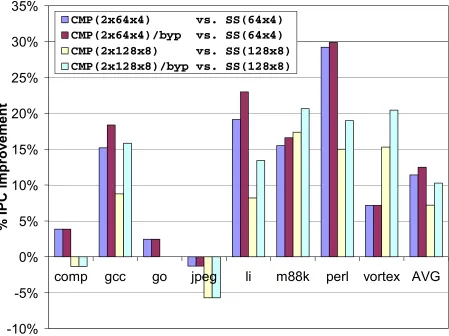
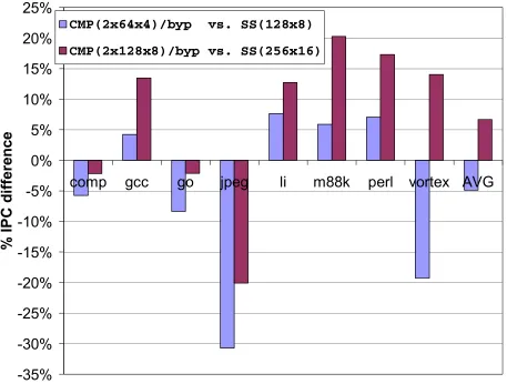
Figure 4-2. Performance improvement using a second processor for slipstreaming... 37
Figure 4-3. Performance of slipstream execution on two small processors vs. performance of conventional non-redundant execution on a single large processor. ... 39
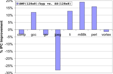
Figure 4-4. Performance improvement of SMT(128x8)/byp over SS(128x8). ... 40
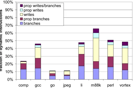
Figure 4-5. Breakdown of instruction removal. ... 41
Figure 4-6. Measuring the relative importance of branch and value prediction benefits... 43
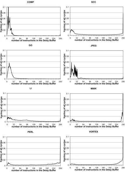
Figure 4-7. Delay buffer occupancy. ... 46
Figure 5-1. Software-based memory duplication. ... 52
Figure 5-2. Hardware-based memory duplication. ... 55
Figure 5-3. Recovery controller operation. ... 59
Figure 5-4. Original slipstream microarchitecture. ... 65
Figure 5-5. New slipstream microarchitecture with hardware-based memory duplication and invalidation-based recovery. ... 65
Figure 5-6. Comparison of duplication methods: performance of SD(rc) and HD(rc) with respect to BASE... 72
Figure 5-7. Comparison of recovery methods for hardware-based memory duplication, averaged across all benchmarks. ... 73
Figure 5-8. Number of referenced stale, self-repair, persistent-stale, and persistent-skipped-write bytes per 1000 instructions... 76
Figure 5-9. Comparison of recovery methods for hardware-based memory duplication, per-benchmark results. 77 Figure 6-1. Unoptimized hardware-based memory duplication for single L1 cache. ... 82
Figure 6-2. Optimized hardware-based memory duplication for single L1 cache: Dirty-Line Duplication. ... 83
Figure 6-3. Speedup of slipstream execution on SMT substrate with two dup. models. ... 85
Figure 6-4. SMT-based slipstream processor with dirty-line duplication is tolerant of IR-mispredictions due to quick recovery... 86
Figure 7-1. Speedup (left) and percentage of intervals that slipstream is active (right) as a function of predicted-ineffectual threshold. (bzip, gap, gcc, jpeg) ... 93
Figure 7-2. Speedup (left) and percentage of intervals that slipstream is active (right) as a function of predicted-ineffectual threshold. (parser, perl, vortex)... 94
Figure 7-3. Slipstream performance with and without management of slipstream execution mode. ... 97
List of Tables
Table 4-1. Benchmarks. ... 33
Table 4-2. Microarchitecture configuration. ... 34
Table 4-3. Branch mispredictions per 1000 instructions. ... 44
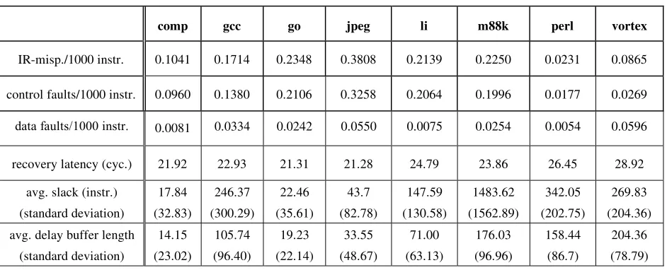
Table 4-4. IR-misprediction rate, recovery latency, slack, and delay buffer length... 45
Table 5-1. Qualitative comparisons of duplication and recovery methods. ... 64
Table 5-2. Microarchitecture configuration. ... 67
Chapter 1 Introduction
The slipstream paradigm [36][41][52] is based on the observation that only a fraction of the
dynamic instruction stream is needed for a program to make full, correct, forward progress. For
example, some instruction sequences have no observable effect. They produce results that are
not subsequently referenced, or results that do not change the state of the machine. And then
there are instruction sequences whose effects are observable, but the effects are invariably
predictable. Computation influencing control flow is the most notable example.
Ineffectual and branch-predictable computation can be exploited to reduce the length of a
running program, speeding it up. Unfortunately, we cannot know for certain which instructions
can be safely skipped until after they have been executed. Constructing a shorter program is
speculative and, ultimately, it must be checked against the full program to verify that it produces
the same overall effect.
Therefore, a slipstream processor concurrently runs two copies of the program, leveraging
either a single-chip multiprocessor (CMP) [34] or a simultaneous multithreading processor
(SMT) [56][59]. (The user program is instantiated twice by the operating system and each copy
has its own context.) One program always runs slightly ahead of the other. The leading program
is called the advanced stream, or A-stream, and the trailing program is called the redundant
stream, or R-stream. Hardware monitors the R-stream and detects (1) instructions that repeatedly
(2) branches whose outcomes are consistently predicted correctly. Future instances of the
ineffectual instructions, branch instructions, and the computation chains leading up to them are
speculatively removed in the A-stream — but only if there is high confidence correct forward
progress can still be made, in spite of removing the instructions.
The reduced A-stream fetches, executes, and retires fewer instructions than it would
otherwise, resulting in a faster program. To verify that the A-stream makes correct forward
progress, all control-flow and data-flow outcomes of the A-stream are passed to the R-stream.
The R-stream checks the outcomes against its own and, if a deviation is detected, the R-stream’s
architectural state is used to selectively repair the A-stream’s corrupted architectural state (an
infrequent event).
A key point is that the R-stream uses the outcomes it is checking as predictions [40]. This
has two advantages.
• First, the R-stream fetches and executes more efficiently due to having near-ideal predictions
from the A-stream. Thus, although the unreduced R-stream retires more instructions, it keeps
pace with the A-stream and the two programs combined finish sooner than a single copy of
the program would. The slipstream processor’s approach of speeding up a single program via
redundancy is analogous to “slipstreaming” in car racing, where two cars race nose-to-tail to
increase the speed of both cars [39].
• Second, by using A-stream outcomes as predictions, the R-stream leverages existing
speculation mechanisms for checking the A-stream. Conventional processors typically have
mechanisms in place to check control flow speculation, and future processors may
An analogy to the slipstream paradigm (and the source of its name) is “slipstreaming” in
stock-car racing (e.g., NASCAR) [39]. At speeds in excess of 190 m.p.h., high air pressure
forms at the front of a race car and a partial vacuum forms behind it. This creates drag and limits
the car’s top speed. A second car can position itself close behind the first (a process called
slipstreaming or drafting). This fills the vacuum behind the lead car, reducing its drag. Likewise,
the trailing car has less wind resistance in front. As a result, both cars speed up by several
m.p.h.: the two combined go faster than either can alone.
In addition to potential performance improvements, slipstreaming provides fault-tolerant
capabilities. The trends of very high clock speeds and very small transistors may make the entire
chip prone to transient faults [45], and there is renewed interest in fault-tolerant architectures for
commodity, high-performance microprocessors [3][38][40].
Slipstream processors provide substantial but incomplete fault coverage; specifically, faults
that affect redundantly-executed instructions are detectable and recoverable. Not all instructions
are redundantly executed because the A-stream is a subset of the R-stream, and this opens up
opportunities for dynamically and flexibly trading performance and fault coverage. A transient
fault, whether it affects the A-stream, the R-stream, or both streams, is transparently detected as
a “misprediction” by the R-stream because the communicated control-flow and data-flow
outcomes from the A-stream will differ from the corresponding outcomes in the R-stream. Fault
detection/recovery is transparent because transient faults are indistinguishable from
prediction-induced deviations.
1.1 Understanding slipstream: Why it works and what are its limits
We present two different interpretations of slipstreaming to better understand the paradigm.
the A-stream. In Section 1.1.2, roles are reversed, where the R-stream is considered to be the
“main” thread and the A-stream “assists” the R-stream. Actually, the two programs in a
slipstream processor are functionally equivalent and mutually beneficial, so either interpretation
is valid.
We next examine limits of the paradigm to motivate removing instructions from the
A-stream before they are fetched. Finally, we consider other ways of reducing the A-A-stream to
highlight the conceptual simplicity of our chosen approach.
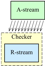
1.1.1 R-stream: A fast checker
The A-stream does not explicitly derive any performance benefit from the R-stream. Rather,
the R-stream checks (and occasionally redirects) the A-stream without slowing it down. This is
possible because checking is inherently parallel [27][40]. The R-stream is not bound by
control-flow and data-control-flow dependences for which the A-stream has produced correct outcomes. As
depicted in Figure 1-1, the R-stream is a fast checking assist to the A-stream [40][41][3].
Checker A-stream
R-stream
Figure 1-1. A fast checking assist to the A-stream.
1.1.2 A-stream: A program-based predictor
Alternatively, the A-stream is a program-based predictor for the R-stream [7][13][43][61].
For example, the A-stream assists the performance of the R-stream by improving its branch
unconfident [19], as shown in Figure 1-2. Confident branch predictions are more likely to be
correct and the corresponding branches and computation feeding the branches are removed from
the A-stream. Confident predictions represent the most accurate predictions; therefore, removing
the computation needed to verify them is sound, and it allows the A-stream to focus instead on
verifying unconfident branch predictions. As a result, many branch mispredictions are resolved
by the A-stream in advance of when the R-stream reaches the same point.
The A-stream also serves as an accurate value predictor [27] for the R-stream. Although only
the results of A-stream-executed instructions are available, the predictions are potentially more
accurate than those provided by conventional value predictors: A-stream “predictions” are
produced by program computation as opposed to being history-based. Perhaps there is some
overlap in what the A-stream provides and what a conventional value predictor could provide.
Results in Section 4.2.3 indicate that some benchmarks (e.g., gcc) benefit primarily from the
short program resolving branch mispredictions in advance; others benefit largely due to value
predictions from the A-stream, and the effect is not always reproducible by conventional value
prediction tables.
A-stream R-stream
Predictor
confident predictions unconfident
predictions verified unverified
Figure 1-2. A combined predictor/program for improving R-stream branch prediction accuracy.
1.1.3 Slipstream limits and the importance of bypassing instruction fetch
Prior research has shown that, in the absence of any resource constraints, performance is
typically limited by mispredicted branches because they serialize execution [25][58]. That is, in
their dependence chains tend to dominate the critical path of the program. The A-stream cannot
reduce this critical path because the dependence chains of mispredicted branches are not safely
removable from the stream — only correctly predicted branches are safely removable. The
A-stream, like a full version of the program, encounters the same mispredictions and resolves them
in program order. Therefore, slipstreaming is not likely to provide performance advantages if
fetch and execution bandwidth are unconstrained.
Understanding slipstreaming’s limitations enables us to focus research efforts on areas that
are likely to pay off. For example, we can reason about the relative importance of bypassing
instruction fetch and execution in the A-stream. Consider a slipstream processor that reduces the
number of instructions executed in the A-stream, but not the number of instructions fetched. The
A-stream runs on one core of a CMP and the R-stream on a second core (for example). As raw
execution bandwidth of both cores is increased, the A-stream starts to lose its edge with respect
to the R-stream. Instruction fetching becomes the bottleneck and, from a practical standpoint, the
A-stream is not truly reduced if the number of fetched instructions is not reduced.
Fortunately, it is possible to bypass even instruction fetching in the A-stream. The A-stream
has a distinct advantage in this regard because raw instruction fetch bandwidth cannot be as
easily extended as raw execution bandwidth, e.g., due to taken branches and branch predictor
bandwidth.
1.1.4 Other ways of reducing the A-stream
One method for reducing the A-stream is removing branch-predictable computation. Another
possibility is removing value-predictable computation. As illustrated in Figure 1-2 in the context
of branch prediction, an overall better value predictor may be possible by combining a
highly value-predictable computation, and the A-stream focuses instead on hard-to-predict
values. The R-stream observes a stream of accurate values comprised of both unverified
confident values and computed values.
However, this approach complicates the mechanism for reducing the stream. For the
A-stream to make correct forward progress, the effects of removed, value-predictable computation
must be emulated by updating the state of the A-stream with values directly, similar to
block/trace/computation reuse [10][15][17] but without the reuse test. This is why we focused
initially on the special cases of ineffectual and branch-predictable computation. This
computation can be literally removed (i.e., replaced with nothing), and only the program counter
needs to be updated to skip instructions.
1.2 Fault tolerance potential
A formal analysis of the fault tolerance of slipstream processors is left for future work. For
now, we informally analyze three key scenarios, shown in Figure 1-3, to better understand
potential fault tolerance. In Figure 1-3, the horizontal lines represent the dynamic instruction
streams of the A-stream and R-stream, with older instructions on the left. For this simple
analysis, we assume only a single fault occurs and that the fault is ultimately manifested as an
erroneous value. A single fault can affect instructions in both streams simultaneously. This is not
a problem because the two redundantly-executed copies of an instruction execute at different
times (time redundancy) [40]; therefore, a single fault that affects both streams will affect
different instructions. Since only one copy of an instruction is affected by a fault, we arbitrarily
choose the R-stream copy, indicated with X’s in Figure 1-3. An X indicates the first erroneous
X R-stream
A-stream
Scenario #1
X Scenario #2
X Scenario #3
Figure 1-3. Transient fault scenarios.
Scenario #1 in Figure 1-3 shows the A-stream and R-stream executing redundantly, i.e., all
instructions overlap and have the same data flow. The fault is detectable because the operands of
the first erroneous instruction differ between A-stream and R-stream. Without more information,
however, the fault is indistinguishable from an IR-misprediction. Under the circumstances, the
processor must assume an IR-misprediction since misspeculation is by far the more common
case. We point out three successively stronger fault tolerance claims.
1. If we assume a fault cannot flip bits in the R-stream’s architectural state, then it does not
matter that faults and Imispredictions are indistinguishable. Recovery succeeds using the
R-stream state. Under this model, faults in the pipeline are transparently recoverable. Faults that
hit the R-stream register file and data cache are unrecoverable, and worse, undetectable as a
fault.
2. If all IR-predictions prior to the first erroneous instruction have been verified, then the
source of error is known to be a fault. Software is invoked to diagnose the system and
perform recovery operations (e.g., restart). But we default back to (1) if there are prior
unresolved IR-predictions.
3. ECC can be used to protect the R-stream register file and data cache, in which case all
transient faults within scenario #1 are transparently recoverable.
Scenario #2 in Figure 1-3 shows a region of the program that is not executed redundantly
(the A-stream bypassed these instructions). A transient fault in the R-stream is undetectable
detected in later, redundantly-executed instructions, the R-stream architectural state is already
corrupted and the system is unaware of this fact.
Scenario #3 shows the A-stream diverging from the R-stream due to an IR-misprediction,
and a transient fault occurs after the divergent point. The IR-misprediction is detected and
subsequent erroneous instructions are squashed before the fault can do damage.
In summary, slipstream processors potentially improve the fault tolerance of the chip. The
system transparently recovers from transient faults affecting redundantly-executed instructions.
1.3 Extending capabilities of CMP/SMT processors
Integrating multiple program contexts on a single chip is an important trend. It is difficult to
conceive of more effective uses for a billion transistors. The slipstream paradigm extends the
capabilities of CMP and SMT substrates. The operating system may flexibly choose among
multiple operating modes based on system and user requirements: high job throughput and
parallel-program performance (conventional SMT/CMP), improved single-program performance
and reliability (slipstream), or highly reliable operation with low performance overhead
(AR-SMT[40] / SRT[38]).
1.4 Contributions
This thesis makes six major contributions, outlined below.
1. First slipstream microarchitecture. A key contribution of this thesis is the development of
the slipstream paradigm and the first slipstream processor. The thesis describes basic
components necessary to facilitate slipstream execution.
2. Understanding slipstream performance and its fundamental limits. Insight is provided
regarding the sources of slipstream performance, and its limitations. This focuses exploration
• A 12% average performance improvement is achieved by harnessing an otherwise
unused, additional processor in a CMP. Programs with little instruction removal are
not sped up at all, whereas programs with upwards of 1/3 instruction removal are
sped up by as much as 30%.
• As more execution bandwidth is made available, slipstream execution provides less
performance improvement. However, if the A-stream is able to bypass instruction
fetching, slipstream retains its edge — because raw instruction fetch bandwidth is not
as easily extended as raw execution bandwidth.
• Slipstream execution using two small superscalar cores often achieves similar IPC as
one large superscalar core, but slipstream has a potentially faster clock and a more
flexible architecture.
• For programs with sufficiently reduced A-streams, slipstream execution on an 8-issue
SMT processor improves performance from 10%-20%.
• For some programs, performance improvement is due to the A-stream resolving
branch mispredictions in advance. Others benefit largely from A-stream value
predictions, and the effect is not always reproducible using conventional value
prediction tables.
3. Method for instruction removal. A method for instruction removal is proposed, including
detecting past-removable instructions in the R-stream and anticipating removable
instructions in the A-stream. We also propose a way to do removal prediction at the
instruction granularity yet remove dependence chains together. A method for removing
instructions before they are fetched is proposed. The thesis focuses on method and not
4. Efficient CMP memory hierarchy
• Duplication. Initially, slipstream execution used a complete copy of the program for
the A-stream. This copy was forked by the operating system (O/S) and took up the
same amount of memory as the R-stream. Using a method called hardware-based
memory duplication, CMP memory usage is reduced to that of a single program,
slipstream execution is transparent to the O/S, and no explicit hardware management
is needed (management is implicit via usual block allocations and replacements).
• Recovery. This thesis contributes several much simpler recovery methods enabled by
hardware-based memory duplication. These methods include invalidating the L1
cache, partially invalidating the L1 cache, and taking advantage of invalidated cache
lines to reduce the penalty of compulsory misses after recovering.
5. Efficient SMT memory hierarchy. A highly efficient memory duplication scheme for a
single-L1-cache SMT processor is developed. Not only does this scheme significantly reduce
L1 cache pressure due to duplication, it also provides a simple zero-penalty method for
repairing A-stream memory state and implicitly prefetches for the R-stream.
6. Management of slipstream execution mode. Slipstream execution does not accelerate all
programs. Even programs that benefit from slipstream may not benefit during all phases. We
have developed very simple hardware support for (1) predicting the effectiveness of
slipstream execution across and within applications and (2) dynamically enabling and
disabling slipstream execution mode. The core mechanisms already exist: The
IR-predictor/IR-detector components conveniently provide continuous feedback (even with the
A-stream disabled), and enabling/disabling the A-stream is procedurally identical to
an operating system to choose between slipstream execution mode and conventional modes
of execution. Alternatively, if the operating system selects slipstream execution mode for an
application, the slipstream management unit can forfeit a spare processor during intervals for
which slipstream is less effective and reclaim it at some later time.
1.5 Thesis
organization
Related work is covered in Chapter 2. The slipstream processor (first contribution) and
instruction removal (third contribution) are covered in Chapter 3. This introductory chapter and
Chapter 4 provide insights regarding slipstream performance (second contribution). Efficient
CMP and SMT memory hierarchies (fourth and fifth contributions) are covered in Chapter 5 and
Chapter 6, respectively. Management of slipstream execution mode (sixth contribution) is
Chapter 2 Related Work
2.1 Basis for reducing the A-stream
Researchers have demonstrated a significant amount of redundancy, repetition, and
predictability in general-purpose programs [10][15][17][26][27][29][31][46][47][57]. This prior
research forms a basis for creating the shorter program in slipstream processors. A technical
report studying the feasibility of reducing programs [41] showed (1) it is possible to ideally
construct significantly reduced programs that produce correct final output, and (2) AR-SMT is a
convenient execution model to exploit this property (AR-SMT is a fault-tolerant
microarchitecture and precursor to slipstream execution, described in Section 2.2).
2.2 Execution models based on hardware multithreading
Advanced-stream/Redundant-stream Simultaneous Multithreading (AR-SMT) [40] is based
on the realization that microarchitecture performance trends and fault tolerance are related. Time
redundancy — running a program twice to detect transient faults — is cheaper than hardware
redundancy, but it doubles execution time. AR-SMT runs the two programs simultaneously [56]
but delayed slightly (via the delay buffer), reducing the performance overhead of time
redundancy. Results are compared by communicating all retired A-stream results to the
R-stream, and the R-stream performs the checks. Here, the R-stream leverages speculation
fetches/executes with maximum efficiency, further reducing the performance overhead of time
redundancy. And the method for comparing the A-stream and the R-stream is conveniently in
place, in the form of misprediction-detection hardware. In summary, AR-SMT leverages the
underlying microarchitecture to achieve broad coverage of transient faults with low overhead,
both in terms of performance and changes to the existing design.
DIVA [3] and SRT [38] are two other examples of fault-tolerant architectures designed for
commodity high-performance microprocessors. DIVA detects a variety of faults, including
design faults, by using a verified checker to validate computation of the complex processor core.
DIVA leverages an AR-SMT technique — the simple checker is able to keep pace with the core
by using the values it is checking as predictions. SRT improves on AR-SMT in a variety of
ways, including a formal and systematic treatment of SMT applied to fault tolerance (e.g.,
spheres of replication).
Tullsen et al. [55][56] and Yamamoto and Nemirovsky [59] proposed simultaneous
multithreading for flexibly exploiting thread-level and instruction-level parallelism. Olukotun et.
al. [34] motivate using chip multiprocessors.
Farcy et al. [13] proposed resolving branch mispredictions early by extracting the
computation leading to branches. Zilles and Sohi [61] similarly studied the computation chains
leading to mispredicted branches and loads that miss in the level-two cache. They suggest
identifying a difficult subset of the program for pre-execution [43][44], potentially prefetching
branch predictions and cache lines that would otherwise be mispredictions and cache misses.
Pre-execution typically involves pruning a small kernel from a larger program region and
running it as a prefetch engine [44]. Roth and Sohi [43] developed a new paradigm called
of work on pre-execution architectures has developed in recent years
[2][4][7][9][28][33][49][62]. Rather than spawn many specialized kernels on-the-fly, our
approach uses a single, functionally complete, and persistent program (A-stream). Slipstream
execution avoids the conceptual and possibly real complexity of forking private contexts, within
which the specialized kernels must run.
Dundas and Mudge [11] proposed run-ahead to improve first-level data cache performance.
Run-ahead enables an in-order pipeline to silently fetch and execute instructions around a stalled
load, exploiting the otherwise idle execution core to generate highly accurate data prefetches.
The only hardware required is an additional register file. Balasubramonian, Dwarkadas, and
Albonesi [4] extend run-ahead to out-of-order pipelines, to reserve a portion of the window for a
future thread. The future thread executes when the primary thread is limited by resource
availability. The future thread is not bound by in-order retirement, so it can examine a much
larger window. Results are communicated to the primary thread via the instruction and data
caches (pre-fetching), instruction reuse buffer (pre-computation), and branch predictor
(resolving branch mispredictions early). The speculative thread is only initiated when the main
thread is stalled, whereas slipstream deploys a redundant program (A-stream).
Speculative multithreading architectures [1][34][48] accelerate a single program by dividing
it into speculatively-parallel threads. The speculation model uses one architectural context and
future threads are spawned within temporary, private contexts, each inherited from the preceding
thread’s context. Future thread contexts are merged into the architectural context as threads
complete. Our speculation model uses redundant architectural contexts, so no forking or merging
is needed. Moreover, there are no dependences between the architecturally-independent threads,
memory mechanisms of the underlying processor are relatively unchanged by slipstreaming
(particularly if there is an existing interface for consuming value predictions at the rename
stage). In contrast, speculative multithreading often requires elaborate inter-thread
register/memory dependence mechanisms.
SSMT [7] runs microthreads simultaneously with an application to optimize its performance.
Microthreads are small routines designed in conjunction with applications and the processor. For
example, microthreads may perform cache prefetching, improve branch prediction accuracy [7],
or optimize exception handling [60].
The DataScalar paradigm [6] runs redundant programs on multiple processor-and-memory
cores to eliminate memory read requests.
2.3 Thread memory management
In this section, memory management strategies of various multithreaded execution models
are described and contrasted with slipstream memory management. References are made to
methods proposed in Chapter 5, which the reader may read first to better appreciate the
following coverage of related work.
2.3.1 Redundant execution
The AR-SMT [40], DIVA [3], and SRT [38] architectures execute two redundant copies of
the program for fault tolerance. AR-SMT uses software-based memory duplication to enable
arbitrary slip between the A-stream and R-stream, limited only by the length of the delay buffer.
SRT merges redundant stores before they are committed, so memory is not duplicated.
However, the SRT design space allows for register duplication, memory duplication, or both.
The initial DIVA implementation does not duplicate register or memory state. However, to
implementations include duplicate register files and/or L1 caches (the L1 caches can be different
sizes) [8]. State of the leading thread is not written back to the L2, although the issue of
replacing modified lines in the L1 cache of the leading thread is not discussed. Preventing stale
references may require that the checker thread signal when it has performed all corresponding
modifications, at which time the leading thread can safely discard its version of the line. On the
other hand, permitting stale references simplifies the hardware, but whole-cache invalidations
would become more frequent and the recovery optimizations developed in this thesis can benefit
the DIVA microarchitecture as well. To the best of our knowledge, this thesis is the first to
propose discarding updates of the leading thread based on the prediction that discarded updates
are likely to be re-created in a timely fashion by the trailing thread [37]. This approach
eliminates explicit management, the prediction is accurate in practice, and correctness is
maintained. Other unique aspects include the invalidate-dirty-line recovery heuristic and the use
of invalidated lines as highly-accurate value predictions for reducing the impact of
recovery-induced misses, both of which are crucial for maximizing performance without the recovery
controller. We also provide insight by characterizing the frequency of references to stale data,
self-repair data, persistent-stale data, and persistent-skipped-write data. Finally, we
implemented hardware-based memory duplication in the context of a POWER4-style memory
hierarchy including considerations for cache coherence between the L1 caches and with the rest
of the system.
2.3.2 Speculative multithreading
Speculative multithreading architectures (e.g., [1][24][34][35][48][50]) accelerate a
sequential program by dividing it into speculative parallel tasks, and concurrently running the
these architectures provide private L1 caches for tasks. Examples include the Multiscalar
Processor with SVC [16], TLDS [50], and MDT [24]. The L1 caches are explicitly managed to
enforce inter-task dependences. In contrast, there are no dependences between the A-stream and
R-stream. Confining the A-stream to its L1 cache occasionally causes A-stream updates to be
lost. Whether the A-stream re-references stale data or updated data depends on whether or not
the R-stream has performed its corresponding store, but this dependence is not enforced.
Therefore, the L1 caches are not explicitly managed in the case of slipstream.
2.3.3 Pre-execution
Speculative Data-Driven Multithreading [43] and other pre-execution architectures
[2][4][7][9][11][13][28][33][49][62] fork specialized threads to prefetch cache misses and
resolve branch mispredictions in advance. A key difference is the use of multiple, short-lived,
specialized threads versus a single, persistent, functionally-complete program (A-stream). This
difference results in very different microarchitectures and, specifically, memory renaming has
evolved differently. Use of the memory hierarchy (e.g., L1 cache or full duplication) is tailored
towards the A-stream’s persistence and completeness. Linking stores directly to loads via an
explicitly-managed memory cloaking table [32], bypassing the memory system entirely, is
tailored towards short-lived dependence-chain-based threads. Many pre-execution architectures
omit stores from the specialized threads altogether because stores do not typically affect their
Chapter 3 Slipstream Microarchitecture
A slipstream processor requires two architectural contexts, one for each of the A-stream and
R-stream, and new hardware for directing instruction-removal in the A-stream and
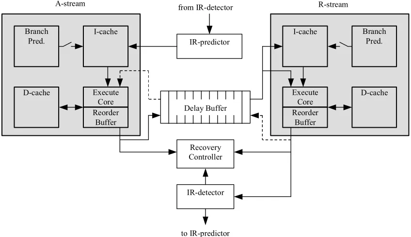
communicating state between the threads. A high-level block diagram of a slipstream processor
implemented on top of a dual-processor chip multiprocessor (CMP) is shown in Figure 3-1,
although an SMT processor might also be used. The shaded boxes show the original processors
comprising the multiprocessor. Each is a conventional superscalar/VLIW processor with a
branch predictor, instruction and data caches, and an execution engine — including the register
file and either an in-order pipeline or out-of-order pipeline with reorder buffer.
Slipstreaming requires four new components.
1. The instruction-removal predictor, or IR-predictor, is a modified branch predictor. It
generates the program counter (PC) of the next block of instructions to be fetched in the
A-stream. Unlike a conventional branch predictor, however, the predicted next PC may reflect
skipping past any number of dynamic instructions that a conventional processor would
otherwise fetch and execute. Also, the IR-predictor indicates which instructions within a
fetched block can be removed after the instruction fetch stage and before the decode/dispatch
stage.
2. The instruction-removal detector, or IR-detector, monitors the R-stream and detects
in the future. The IR-detector conveys to the IR-predictor that particular instructions should
potentially be skipped by the A-stream when they are next encountered. Repeated indications
by the IR-detector build up confidence in the IR-predictor, and the predictor will remove
future instances from the A-stream.
3. The delay buffer is used to communicate control-flow and data-flow outcomes from the
A-stream to the R-A-stream [40].
4. The recovery controller maintains the addresses of memory locations that are potentially
corrupted in the A-stream context. A-stream context is corrupted when the IR-predictor
removes instructions that should not have been removed. Unique addresses are added to and
removed from the recovery controller as stores are processed by the A-stream, the R-stream,
and the IR-detector. The current list of memory locations in the recovery controller is
sufficient to recover the A-stream memory context from the R-stream’s memory context.
The register file is repaired by copying all values from the R-stream’s register file.
Branch
Pred. I-cache
D-cache Execute
Core Reorder
Buffer
Branch Pred. I-cache
D-cache Execute
Core Reorder
Buffer IR-predictor
Delay Buffer
Recovery Controller
IR-detector from IR-detector
A-stream R-stream
to IR-predictor
The diagram in Figure 3-1 shows the A-stream on the leftmost core and the R-stream on the
rightmost core. This is arbitrary and does not reflect specializing the two cores. A real design
would have one core that flexibly supports either the A-stream or R-stream. In any case, there is
a clear symmetry that makes designing a single core natural. In both cores, there is an interface
to the fetch unit that overrides the conventional branch predictor, indicated symbolically with an
open switch and a second interface to the fetch unit. Likewise, both cores show symmetric
interfaces to and from the execution pipeline.
3.1 Creating the shorter program
3.1.1 Base IR-predictor
The IR-predictor resembles a conventional branch predictor. In this thesis, the IR-predictor is
indexed identically to a gshare predictor [30], i.e., an index is formed by XORing the PC and the
global branch history bits. Each table entry contains information for a single dynamic basic
block.
• Tag: This is the start PC of the basic block and is used to determine whether or not the entry
contains information for the desired block.
• 2-bit counter: If the block ends in a conditional branch, the 2-bit counter predicts its
direction.
• Confidence counters. There is a resetting confidence counter [19] for each instruction in the
block. The counters are updated by the IR-detector: a counter is incremented if the
corresponding instruction is detected as removable, otherwise the counter is reset to zero. If a
counter is saturated, then the corresponding instruction will be removed from the A-stream
Every fetch cycle, the IR-predictor supplies a branch prediction and an instruction-removal
bit vector to the A-stream fetch unit. The branch prediction is used to select a PC for the next
fetch cycle; potential target PCs are stored within existing structures of the processor, e.g.,
pre-decoded targets in the instruction cache or branch target buffer.
The instruction-removal bit vector reflects the state of the confidence counters for the basic
block being fetched. A bit is set in the vector if the corresponding confidence counter is
saturated, and this directs the fetch unit to remove the corresponding instruction from the
A-stream. Thus, although all instructions in the basic block are fetched, potentially many
instructions are removed before the decode stage of the pipeline.
In Figure 3-1, the IR-predictor is shown as a new component outside the processor core that
overrides the conventional branch predictor. Alternatively, since the IR-predictor is built on top
of a conventional branch predictor, the core’s predictor and the IR-predictor may be integrated.
3.1.2 Improved IR-predictor: Bypassing instruction fetch
With the base IR-predictor described in Section 3.1.1, the A-stream is not reduced in terms
of the number of instructions fetched. Only the number of instructions executed is reduced. If
execution bandwidth is relatively unconstrained, then the A-stream will not be effectively
reduced.
The A-stream is more effective if fewer fetch cycles are expended on it than on the full
program. In Figure 3-2, we show an example of how the number of fetch cycles can potentially
be reduced. Four basic blocks, labeled A through D, are to be predicted and fetched. The
corresponding table entries in the IR-predictor are shown; darker shaded entries indicate that all
of the confidence counters are saturated and the entire basic block is predicted for removal. The
cycles, the instruction cache fetches instructions and then throws them all away (basic blocks B
and C). Clearly, only two fetch cycles are required, but it is not known in advance that
instruction fetching of blocks B and C can be bypassed.
A
B
C
D
improved IR-predictor
A
B
C
D base IR-predictor
Figure 3-2. Reducing fetch cycles in the A-stream.
Interestingly, the effect we want to produce — bypassing basic blocks — is the same effect
produced by taken branches. The improved IR-predictor shown on the right-hand side of Figure
3-2 exploits the analogy. The improved predictor “converts” the branch terminating block A into
a taken branch whose target is block D. Below, we consider two possible ways to implement this
conversion.
• Two additional pieces of information are stored in block A’s table entry. First, the predicted
directions of any bypassed branches must be stored, in this case, the predicted directions of
the branches in blocks B and C. The reason is that all control flow information must be
pushed onto the delay buffer to be consumed by the R-stream, in spite of partially bypassing
instruction fetching in the A-stream. Second, a target address must be stored, in this case, the
start PC of block D. The target address overrides the next PC computation performed by the
address) is accumulated for block A’s entry as the IR-detector sequentially updates the
entries of blocks B, C, and D.
• Effectively, the branch terminating block A is now a multi-way branch. It has more potential
targets than its original taken and fall-through targets because it inherits the targets of
skipped blocks. The processor’s branch target buffer may be modified to store multiple
targets per branch. Now, dynamically-created target addresses do not have to be stored in the
IR-predictor. The bypassed predictions still need to be stored and, conveniently, this path
information is sufficient to select the appropriate target address from the branch target
buffer.
3.1.3 IR-detector
The IR-detector consumes retired R-stream instructions, addresses, and values. The
instructions are buffered and, based on data dependences, circuitry among the buffers is
dynamically configured to establish connections from consumer to producer instructions. In
other words, a reverse dataflow graph (R-DFG) is constructed. The graph is finite in size, so the
oldest instructions exit the graph to make room for newer instructions. Removal information for
exiting instructions is used to update the IR-predictor.
As new instructions are merged into the R-DFG, the IR-detector watches for any of three
triggering conditions for instruction removal. Triggering conditions are unreferenced writes (a
write followed by a write to the same location, with no intervening read), non-modifying writes
[26][29][31][57] (writing the same value to a location as already exists at that location), and
correctly-predicted branch instructions. When a triggering condition is observed, the
back-propagate the selection status to predecessor instructions. Predecessors may also be selected if
certain criteria (described later) are met.
The IR-detector is shown in Figure 3-3. A single R-DFG is shown, however, the buffering
could be partitioned into multiple smaller R-DFGs. The latter approach reduces the
size/complexity of each individual R-DFG but still allows a large analysis scope for killing
values (observing another write to the same location).
FIFO buffer Ope rand
Rename Table (ORT)
valid new instruction,
R-bit, B-bit merge
• kill instructions
• select unreferenced writes, non-modifying writes, and correctly-predicted branches for removal
update IR-predictor RDFG
explicit back-propagation
ref value
producer
Figure 3-3. IR-detector.
The operand rename table (ORT) in Figure 3-3 is similar to a conventional register rename
table but it can track both memory addresses and registers. A single entry of the operand rename
table is shown in Figure 3-3. To merge an instruction into the R-DFG, each source operand is
checked in the ORT to get the most recent producer of the value (check the valid bit and
producer field). The instruction uses this information to establish connections with its producer
instructions, i.e., set up the back-propagation logic (if the buffering is partitioned into smaller
R-DFGs, connections cannot be made across partition boundaries). The ref bit is set for each source
location, then the corresponding rename table entry is checked to detect
non-modifying/unreferenced writes and to kill values, as follows.
1. If the valid bit is set and the current instruction produced the same value as indicated in the
value field, then the current instruction is a non-modifying write. The current instruction is
selected for removal as it is merged into the R-DFG. No fields are updated in the rename
table entry since the old producer remains “live” in this case.
2. If the valid bit is set and the new and old values do not match, then the old producer
indicated by the producer field is killed. Furthermore, if the ref bit is not set, then the old
producer is an unreferenced write and is selected for removal. Finally, all fields in the
rename table entry are updated to reflect the new producer.
Correctly predicted branch instructions (indicated by the B-bit in Figure 3-3) are selected for
removal when they are merged into the R-DFG.
Finally, any other instruction x may be selected for removal via the R-DFG back-propagation
circuitry, if three conditions are met.
1. All of x’s dependent instructions must be known, i.e., x’s production(s) must be killed by
other production(s).
2. All of x’s dependent instructions must be selected for removal.
3. All of x’s dependent instructions must have been removed by the IR-predictor this time
around. (The R-bit in Figure 3-3 indicates whether or not an instruction was removed by the
IR-predictor this time around.)
When a basic block becomes the oldest basic block in the analysis scope, the corresponding
entry for that basic block is updated in the IR-predictor, i.e., confidence counters are
The third back-propagation condition, highlighted above and called the R-bit criterion, is a
major innovation. The R-bit criterion ensures a producer’s counter saturates only after all
consumers’ counters saturate. This prevents recurring IR-mispredictions caused by (1) multiple
consumers on different control-flow paths and (2) IR-predictor aliasing that causes a consumer’s
counter to reset.
The first case is shown in Figure 3-4. Nodes are instructions, solid arrows are control-flow
edges, and dashed arrows are data dependences. A single producer instruction has consumers on
both paths after the branch instruction. Thus, the producer is back-propagated to along two
separate control-flow paths. If the intervening branch alternates fairly often, then the
back-propagated instruction's confidence can saturate (shown as a wholly-shaded node) before either
of the consumer instructions is removable (shown as the three-quarter-shaded nodes). This
results in multiple IR-mispredictions until the confidence counters of all consumers become
saturated, or until one of the consumer instructions becomes effectual (resetting the confidence
counter of the back-propagated instruction). By requiring an instruction to be actually removed
before back-propagation (R-bit criterion), the back-propagated instruction doesn't even begin to
get confident until its consumers are removed.
A similar situation occurs when a consumer’s basic block is displaced from the IR-predictor
by aliasing, resetting its removal information. If the producer's block is not aliased, it is still
removable, resulting in the same scenario as before (producer’s counter saturated and
consumer’s counter not saturated). Back-propagation based on the R-bit criterion will likely
generate a single IR-misprediction from the aliasing but will correctly reset the back-propagated
The significance of the R-bit method is that it manages confidence counters individually, yet
implicitly synchronizes the counters of arbitrarily distant producers and consumers.
Recently, Koppanalil and Rotenberg [22][23] reduced the complexity of the IR-detector
substantially with the realization that back-propagated instructions are no different from
unreferenced writes, therefore back-propagation can be achieved implicitly via the ORT. This
eliminates the R-DFG component in Figure 3-3. The method described above (the R-bit criterion
in particular) is a key enabler for implicit back-propagation.
branch
Figure 3-4. Example showing the need for synchronizing counters.
3.2 Delay
buffer
The delay buffer is a simple FIFO queue that allows the A-stream to communicate
control-flow and data-control-flow outcomes to the R-stream. The A-stream pushes both a complete history of
branch outcomes and a partial history of operand values onto the delay buffer. This is shown in
Figure 3-1 with a solid arrow from the reorder buffer of the A-stream (left-most processor) to
the delay buffer. Value history is partial because only a subset of the program is executed by the
A-stream. Complete control history is available, however, because the IR-predictor predicts all
branches even though the A-stream may not fetch all instructions (Section 3.1.2).
The R-stream pops control-flow and data-flow information from the delay buffer. This is
shown in Figure 3-1 with solid arrows from delay buffer to the instruction cache and execution
to the instruction cache to direct instruction fetching. Source operand values and load/store
addresses from the delay buffer are merged with their respective instructions after the
instructions have been fetched/renamed and before they enter the execution engine. To know
which values/addresses go with which instructions, the delay buffer also includes a single bit per
dynamic instruction indicating which instructions were skipped by the A-stream (for which there
is no data-flow information available).
3.3 IR-misprediction
recovery
An instruction-removal misprediction, or IR-misprediction, occurs when A-stream
instructions were removed that should not have been. The A-stream has no way of detecting the
IR-misprediction, therefore, it continues instruction retirement and corrupts its architectural
state. Two things are required to recover from an IR-misprediction. First, the IR-misprediction
must be detected and, second, the corrupted state must be pin-pointed for efficient recovery
actions.
IR-mispredictions are detectable by the R-stream because either the control-flow or
data-flow outcomes from the delay buffer will not match its redundantly computed outcomes. In
other words, Imispredictions eventually surface as branch or value mispredictions in the
R-stream.
Some IR-mispredictions take awhile to cause any visible symptoms in the A-stream. For
example, a store may be removed incorrectly and the next load to the same location may not
occur for a very long time. The IR-detector can detect these IR-mispredictions much sooner by
comparing its computed removal information against the corresponding predicted removal
information — if they differ, computation was removed that should not have been. Thus, the
However, we found that checking for IR-mispredictions in the IR-detector provides little benefit
and that waiting for IR-mispredictions to be detected by the R-stream yields the best
performance.
When an Imisprediction is detected, the reorder buffer of the stream is flushed. The
R-stream architectural state now represents a precise point in the program to which all other
components in the processor are re-synchronized. The IR-predictor is backed up to the precise
program counter, the delay buffer is flushed, the reorder buffer of the A-stream is flushed, and
the A-stream’s program counter is set to that of the R-stream.
All that remains is restoring the corrupted register and memory state of the A-stream so it is
consistent with the stream. Because register state is finite, the entire register file of the
R-stream is copied to the A-R-stream register file. The movement of data (both register and memory
values) occurs via the delay buffer, in the reverse direction, as shown with dashed arrows in
Figure 3-1.
The recovery controller receives control signals and the addresses of store instructions from
the A-stream, the R-stream, and the IR-detector, as shown in Figure 3-1. The control signals
indicate when to start or stop tracking a memory address (only unique addresses need to be
tracked). After detecting an IR-misprediction, stores may either have to be “undone” or “done”
in the A-stream.
• The recovery controller tracks addresses of stores retired in the A-stream but not yet retired
in the R-stream. After detecting an IR-misprediction, these A-stream stores must be
“undone” since the R-stream has not yet performed the companion, redundant store.
• The recovery controller tracks addresses of stores retired in the R-stream and skipped in the
IR-misprediction is detected, all unverified, predicted-ineffectual stores are “done” in the
Chapter 4 Evaluation
For the experiments in this chapter, the memory system is somewhat idealized to isolate the
performance of slipstream execution disregarding the effects of full memory duplication. L1
instruction and data caches are modeled but the L2 cache is infinite. The memory hierarchy is
modeled in significant detail in Chapter 5, which investigates various slipstream memory
management alternatives.
4.1 Simulation
environment
We developed a detailed execution-driven simulator of a slipstream processor. The simulator
faithfully models the architecture depicted in Figure 3-1 and outlined in Chapter 3: the A-stream
produces real, possibly incorrect values/addresses and branch outcomes, the R-stream checks the
A-stream and initiates recovery actions, A-stream state is recovered from the R-stream state, etc.
The simulator itself is validated via a functional simulator run independently and in parallel with
the detailed timing simulator [48][42]. The functional simulator checks retired R-stream
control-flow and data-control-flow outcomes.
The Simplescalar [5] compiler and ISA are used. We use the SPEC95 integer benchmarks
Table 4-1. Benchmarks.
benchmark input dataset dynamic instruction count
compress 40000 e 2231 124 million
gcc cccp.i -o cccp.s 265 million
go 9 9 133 million
jpeg vigo.ppm 166 million
li test.lsp (queens 7) 202 million
m88ksim -c < ctl.in (dcrand.big) 121 million
perl scrabble.pl < scrabble.in 108 million
vortex vortex.in (persons.250) 101 million
Microarchitecture parameters are listed in Table 4-2. The top half of the table lists
parameters for individual processors within a CMP or, alternatively, a single SMT processor.
The bottom half describes the four slipstream components. A large IR-predictor is used for
accurate instruction removal. The removal confidence threshold is 32. The IR-detector has a
scope of 256 instructions and the R-DFG is unpartitioned. The delay buffer stores 256
instructions (data flow buffer) and 4K branch predictions (control flow buffer). The recovery
controller tracks any number of store addresses, although we observe not too many outstanding
addresses in practice. The recovery latency (after the IR-misprediction is detected) is 5 cycles to
startup the recovery pipeline, followed by 4 register restores per cycle, and lastly 4 memory
Table 4-2. Microarchitecture configuration.
single processor core size/assoc/repl = 64KB/4-way/LRU line size = 16 instructions
2-way interleaved instruction cache
miss penalty = 12 cycles
size/assoc/repl = 64KB/4-way/LRU line size = 64 bytes
data cache
miss penalty = 14 cycles
reorder buffer: 64, 128, or 256 entries
dispatch/issue/retire bandwidth: 4-/8-/16-way
n fully-symmetric function units (n = issue b/w) superscalar core
n loads/stores per cycle (n = issue b/w) address generation = 1 cycle
memory access = 2 cycles (hit) integer ALU ops = 1 cycle execution latencies
complex ops = MIPS R10000 latencies new components for slipstreaming 220 entries
gshare-indexed (16 bits of global branch history) block size = 16
16 confidence counters per entry IR-predictor
confidence threshold = 32
IR-detector R-DFG = 256 instructions, unpartitioned
data flow buffer: 256 instruction entries delay buffer
control flow buffer: 4K branch predictions # of outstanding store addr. = unconstrained
recovery controller
recovery latency (after IR-misp. detected): • 5 cycles to start up recovery pipeline
4.2 Results
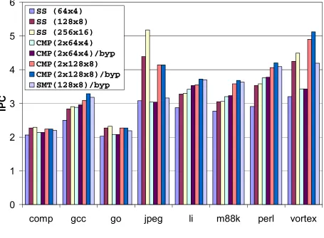
4.2.1 Slipstream performance results
In this section, we compare the performance of eight models. Three are superscalar
configurations (SS). Four are chip-multiprocessor configurations (CMP) with slipstreaming. One
is a simultaneous multithreading configuration (SMT) with slipstreaming.
• SS(64x4): A single 4-way superscalar processor with 64 ROB entries.
• SS(128x8): A single 8-way superscalar processor with 128 ROB entries.
• SS(256x16): A single 16-way superscalar processor with 256 ROB entries.
• CMP(2x64x4): Slipstreaming on a CMP composed of two SS(64x4) cores.
• CMP(2x64x4)/byp: Same as previous, but A-stream can bypass instruction fetching.
• CMP(2x128x8): Slipstreaming on a CMP composed of two SS(128x8) cores.
• CMP(2x128x8)/byp: Same as previous, but A-stream can bypass instruction fetching.
• SMT(128x8)/byp: Slipstreaming on SMT, where the SMT is built on top of SS(128x8).
For consistent comparisons, the same (gshare-based) IR-predictor provides branch
predictions in all of the processor models, and the base superscalar processor models ignore the
instruction-removal information. Performance is measured in retired instructions-per-cycle
(IPC). For slipstream models, IPC is computed as the number of retired R-stream instructions
(i.e., the full program, counted only once) divided by the number of cycles required for both the
A-stream and R-stream to complete (total execution time).
IPC performance of the eight models is shown in Figure 4-1. The first conclusion is a
slipstream processor can exploit a second, otherwise unused processor to significantly improve
than using only a single SS(64x4) processor. And CMP(2x128x8) performs on average 7%
better than using only a single SS(128x8) processor. Slipstreaming degrades performance in
jpeg, by 1% and 5% for CMP(2x64x4) and CMP(2x128x8), respectively. Jpeg’s A-stream is not
reduced much and jpeg is already quite parallel; IR-mispredictions cause an overall degradation.
0
1
2
3
4
5
6
comp
gcc
go
jpeg
li
m88k
perl
vortex
IPC
SS (64x4) SS (128x8) SS (256x16) CMP(2x64x4) CMP(2x64x4)/byp CMP(2x128x8) CMP(2x128x8)/byp SMT(128x8)/byp