Image Depth Extraction Algorithm Using
Wavelet Coefficients and Dense
Representations
Aswathy S Bhanu1, Renjith R J2
P.G. Student, Dept. of Electronics and Communication Engineering, SCT College of Engineering, Kerala, India1 Assistant Professor, Dept. of Electronics and Communication Engineering, SCT College of Engineering, Kerala, India2
ABSTRACT:Defining depth of an arbitrary image is a sophisticated task. Without knowing the cues for absolute depth
measurement, the distance between observer and scene cannot be obtained accurately. Many methods are employed for calculating image depth map, but most of them cannot be used for dynamic scenes and scenes which are invariant to rotation and scale.The paper aims to illuminate the way to 3D modelling by generating the depth map of an image. The technique uses wavelet coefficients correlation to generate the depth map of arbitrary images automatically. The method includes 3 steps; matched image selection, image warping and optimization. By extracting the wavelet coefficient features, 3 matched images are selected for warping using SIFT flow algorithm. Optimization eliminates inaccuracies in the inferred depth map by spatial smoothening. Result produces depth map comparable to the sensor developed depth maps.
KEYWORDS: Depth extraction, Wavelet coefficient correlation, SIFT flow, Warping, Optimization.
I. INTRODUCTION
Depth of an image is defined as the information which represents the relative distances of the objects in the 2D image content. The generation of accurate and natural depth is of great importance and low computational complexity is also required.This paper proposes a depth map generation algorithm which automatically generates the depth maps from images using wavelet coefficient correlation [6].
Several methods have been proposed to directly estimate the depth of image pixels. One approach is to use the information contained inside of an image, known as depth cues, to determine pixel depth. Successful methods generally utilize machine learning techniques to estimate the depth from training data [1]-[3]. Another approach is to use the geometry that occurs when a single scene is imaged by multiple cameras. These methods are able to extract the 3D structure of a scene very accurately from image collections [4]. [5] Perform a pseudo-SFM on animage to obtain a sparse depth estimate and interpolate to generate a sense depth map.
The rest of the paper is organized as follows: we introduce the concept of depth extraction algorithm in section II. In section III, we show the experimental results and the analysis of obtained results. After the analysis of results obtained, we conclude the paper in section IV.
Fig.1 Pipeline for depth extraction algorithm
II. DEPTH EXTRACTION ALGORITHM
A. Feature Extraction
To extract features of an image, the image is decomposed into two levels in the wavelet domain. The joint probability density of each sub-band’s difference from adjoining coefficients in the horizontal, vertical and diagonal directions is calculated using intra wavelet sub-band correlation coefficients. From [9], it was shown that features such as entropy, energy and moment of inertia have better statistical properties. So, in this work we used entropy and energy as the main features.
1. Wavelet Decomposition
Wavelet transform was developed based on the Fourier transform, but they differ from two considerable differences. To represent the signal characteristics, Fourier transform uses separate time domain or frequency domain,
RGBD IMAGE DATABASE RGB IMAGE (INPUT)
WAVELET FEATURE EXTRACTION
SELECTION OF 3 MATCHED IMAGES (RGBD IMAGES)
PREPROCESSING
SIFT FLOW WARPING OF MATCHED IMAGES
OPTIMIZATION
whereas the wavelet transform uses a combination of both time and frequency domain. First step of feature extraction process is wavelet decomposition. The image is decomposed into two or three levels using the specific decomposition process. Fig. 2 represents the 2 level decomposition of an image.
Fig. 2 Two level decomposition of an image
If the scaling and wavelet functions are separable, the summation can be decomposed into two stages. First step is along the x-axis and then calculate along the y-axis. A schematic diagram is shown in Fig. 2. The two dimensional signal (usually image) is divided into four bands: LL (left-top), HL (right-top), LH (left-bottom) and HH (right-bottom). The HL band indicated the variation along the x-axis while the LH band shows the y-axis variation. Fig. 2 shows the decomposition of an image. The power is more compact in the LL band.
Fig. 3 Relationship between pixel blocks of 4 adjacent pixels
In the wavelet domain, subtracting two adjacent wavelet coefficients reflects the relationship between pixel blocks constructed of four adjacent pixels up and down in the spatial image domain, as shown in Fig. 3.Suppose that N1 and
N2 are two adjacent sub-band wavelet coefficients after the Haar wavelet transform and that they are constructed from
the four adjacent pixels n11, n12, n21, n22 and n13, n14, n23, n24 in the spatial domain, then:
= 1 2 ( + ) + 1 2 ( + ) (1)
= 1 2 ( + ) + 1 2 ( + ) (2)
These equations shows that the wavelet coefficient difference reflects on relationship between the two pixel blocks which composed of four pixels nij in the spatial domain as well as the relationship between these two coefficients.
2. Co-Occurrence Matrix Calculation
In the wavelet domain, the weak correlation among the intra-wavelet sub-band coefficients reflects the properties of image texture and edge structure. The joint probability density function of the intra-wavelet sub-band’s difference elements can be described using the correlation statistics of the intra-wavelet sub-band. The joint probability density function of the intra-wavelet sub-band reflected in the spatial domain represents the internal characteristics of the image block. After Haar wavelet transform, let N3 and N4 are two adjacent vertical sub-band wavelet coefficients and that they
are constructed from the four adjacent pixels n11, n12, n21, n22 and n13, n14, n23, n24 in the spatial domain:
= 1 2 ( − ) + 1 2 ( − ) (4)
= 1 2 ( − ) + 1 2 ( − ) (5)
= − = 1 2 ( − ) + 1 2 ( − ) − 1 2 ( − ) + 1 2 ( − ) (6)
From eqs. (3) and (4) – (6), the joint probability density of the intra-wavelet sub-band coefficients M1 and M2 in the
spatial domain reflects the correlation between the two pixel blocks.
Entropy: The entropy of the co-occurrence matrix in a spatial domain is a measure of image clutter. In a gray scale image, if the image has more texture, which shows that entropy value becomes higher; if less, the value becomes lower. The entropy can be expressed as follows:
= − ( , ) log( ( , )) (7)
Energy: The energy of the co-occurrence matrix in a spatial domain is also known as the second angular moment. If
the image pixels are distributed more evenly, there are many zero elements in the co-occurrence matrix, and the energy value is higher. The energy can be expressed as:
= − ∑ ∑ ( , ) (8)
3. Feature Extraction Algorithm
Input: Input image whose depth to be extracted.
Output: Best 3 matched RGB images from the RGBD database.
Step 1: Image decomposition. The RGBD images and the input image should be decomposed into three levels in a
wavelet domain. Thus all 12-wavelet sub-bands including the original image should be obtained.
Step 2: Calculate the difference between each pair of adjacent coefficients in the first- and second-level sub-bands
including the input in the horizontal, vertical, and diagonal directions.
images.
B. SIFTFLOW WARPING
1. Pre-processing
Pre-processing is the initialization step of warping. We compute the prior information about the depth map by averaging matched 3 depth images in our database. This will guide the inference when pixels have little or no influence from other terms.
2. SIFT Flow Algorithm
Dense SIFT Descriptors and Visualization: SIFT is a local descriptor to characterize local gradient information. In
[10], SIFT descriptor is a sparse feature representation that consists of both feature extraction and detection. In [7], only use the feature extraction component. For every pixel in an image, we divide its neighbourhood (e.g., 16 x 16) into a 4 x 4 cell array, quantize the orientation into 8 bins in each cell, and obtain a 4 x 4 x8 128-dimensional vector as the SIFT representation for a pixel. This per-pixel SIFT descriptor is called as SIFT image.To visualize SIFT images, we compute the top three principal components of SIFT descriptors from a set of images and then map these principal components to the principal components of the RGB space.
Matching Objective: We have designed an objective function to estimate SIFT flow from two SIFT images. We want
SIFT descriptors to be matched along the flow vectors, and the flow field to be smooth, with discontinuities agreeing with object boundaries. Based on these two criteria, the objective function of SIFT flow is formulated as follows: Let p=(x,y) be the grid coordinate of images and w(p)=(u(p),v(p)) be the flow vector at p. We only allow u(p) and v(p) to be integers and we assume that there are L possible states for u(p) and v(p), respectively. Let s1 and s2 be two SIFT
images that we want to match. Set ԑ contains all the spatial neighbourhoods. The energy function for SIFT flow is defined as:
( ) =∑ (|| ( )− ( + ( )|| , t)+∑ (|u( )| + |v( )|) +
∑( , )∈ԑ ( |u( )−u( )|, d)+ ( |u( )−u( )|, d) (9)
Coarse-to-Fine Matching Scheme: In SIFT flow, a pixel in one image can literally match to any pixels in the other
image. To address the performance drawback, we designed a coarse-to-fine SIFT flow matching scheme that significantly improves the performance. The basic idea is to roughly estimate the flow at a coarse level of image grid, then gradually propagate and refine the flow from coarse to fine.
3. Warping
In dense representation, correspondence is established at the pixel level in the two images. Using dense correspondence we can easily warp one image to the other. This process is known as warping. Pixel to pixel correspondence is achieved through SIFT flow, which matches per pixel SIFT features to estimate dense scene alignment. Using this, we estimate warping functions for each candidate image, which map pixel locations from a given matched image’s domain to pixel locations in the input’s domain. The warping functions can be one to many.
C. Optimization
infer. We have to minimize
( ) =∑∈ ( ) + ( ) + ( ) + log( )(10)
where Z is the normalization constant of the probability, and and are parameters. For a single image, objective contains three terms: data ( ), spatial smoothness ( ) and prior ( ).
Eqn [10] requires an unconstrained, non-linear optimization, and use iteratively reweighted least squares to minimize the objective function. Here we have chosen IRLS because it is a fast alterative for solving unconstrained, nonlinear minimization problems. IRLS works by approximating the objective by a linear function of the parameters, and solving the system by minimizing the squared residual, it is repeated until convergence.
III.EXPERIMENTAL RESULTS AND ANALYSIS
In this section, we show the experimental results involving single image depth extraction.The experiments were implemented on a 1.8GHz Intel Core i5 PC with 4GB memory, running under Windows 8. We evaluated our algorithm on the Make3D single image RGBD dataset. The Make3D dataset contains 534 images with corresponding depth maps, partitioned into 400 training images and 134 test images. All the images were resized to 460×345 pixels in order to preserve the aspect ratio of the original images. Since the true focal length of the camera is unknown, we assume a reasonable value of 500 for the resized images.
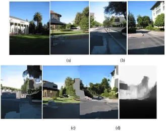
By extracting the wavelet coefficient features of input as well as dataset images, obtained three maximum matched RGB images. These matched images are warped to align them with the input image after pre-processing using the prior depth information. Warping is also introduced to the matched image depth map. Warped depth map is optimized and after performing 10 IRLS iteration, the desired inferred depth map is obtained. The results are shown in fig. 4.
(a) (b)
(c) (d)
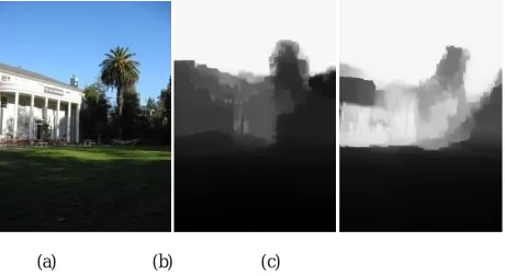
In order to find the accuracy of the obtained output depth map, an image with ground truth depth (sensor developed) is given as the input image. The sensor developed depth is compared with the depth obtained from our depth extraction algorithm. Fig. 5 shows the comparison of ground truth depth to our inferred depth map. Result shows that the depth obtained from our algorithm has 86% accuracy. The depth extraction algorithm using wavelet coefficients only take 297.56 s to extract features over the 400 images of Make3D dataset. Thus, we inferred that our method has better accuracy and take lower computation time than the previous methods.
(a) (b) (c)
Fig. 5 Comparison with the ground truth (a) Input image,(b) Ground truth depth, (c) Inferred depth.
IV.CONCLUSION
We have demonstrated a fully automatic technique to extract the depth map of single images and dynamic scenes. Our depth extraction technique is novel in that we use a wavelet coefficient correlation method, which gives qualitatively good results. Runtime of our proposed method is quite fast, for a purely MATLAB implementation. We obtained an accuracy of 86% when our inferred depth is compared with the ground truth depth. The issue which we are looking to improve is the extension of work to extract the depth of the video sequences.
V. ACKNOWLEDGEMENT
For the successful completion of this paper, there are people behind the screen who contribute a great deal. I take this opportunity to express my sincere and profound gratitude to my thesis guide,Mr Renjith R J (Assistant Professor, Department of Electronics and Communication) for his expert advice, suggestions and encouragement. I wouldalso like to thank my P G coordinator, Mr. Libish T M (Associate Professor, Department of Electronics and Communication) for his valuable support and guidance. I would also like to extend my gratitude to my family for their cooperation in all measure. Above all, I would like to thank the Almighty for his immeasurable blessings showered upon me to make this venture a great success.
REFERENCES
[1] J. Konrad, M. Wang, and P. Ishwar, “2d-to-3d image conversion by learning depth from examples,” in Computer Vision and Pattern Recognition Workshops (CVPRW), 2012 IEEE Computer Society Conference on, june 2012, pp. 16 –22.
[2] Z. Zhang, Y. Wang, T. Jiang, and W. Gao, “Stereoscopic learning for disparity estimation,” in Circuits and Systems (ISCAS), 2011 IEEE International Symposium on, may 2011, pp. 365 –368.
[3] A. Saxena, M. Sun, and A. Ng, “Make3d: Learning 3d scene structure from a single still image,” Pattern Analysis and Machine Intelligence, IEEE Transactions on, vol. 31, no. 5, pp. 824 –840, may 2009.
[4] N. Snavely, I. Simon, M. Goesele, R. Szeliski, and S. Seitz, “Scene reconstruction and visualization from community photo collections,” Proceedings of the IEEE, vol. 98, no. 8, pp. 1370 –1390, aug. 2010.
[5] R. Rzeszutek and D. Androutsos, “Efficient Automatic Depth Estimation for Video,” DSP2013
[7] Ce Liu, Jenny Yuen and Antonio Torralba, “SIFT Flow: Dense Correspondence across Scenes and Its Applications,” IEEE transactions on pattern analysis and machine intelligence, vol. 33, no. 5, may 2011
[8] Kevin Karsch, Ce Liu and Sing Bing Kang, “DepthTransfer: Depth Extraction from Video Using Non-Parametric Sampling,” IEEE Transactions On Pattern Analysis And Machine Intelligence, Vol. 36, No. 11, November 2014
[9] Andrea B and Flavio P.,” An investigation of the textural characteristics associated with gray level co-occurrence matrix statistical parameters”. IEEE Transactions on Geosciences and Remote Sensing 1995; 33(3): 293–304.
[10] D.G. Lowe, “Object Recognition from Local Scale-Invariant Features,” Proc. IEEE Int’l Conf. Computer Vision, pp. 1150-1157, 1999.
BIOGRAPHY
Aswathy S Bhanu1 is currently pursuing the M.Tech. degree in Signal Processing with the Department of Electronics and Communication Engineering, SCT College of Engineering, Kerala, India. She received the B. Tech degree from the Cochin University of Science And Technology, Kerala in 2013 in Electronics and Communication Engineering. Her research interests include signal processing, image processing, and video processing.