ABSTRACT
LOKITZ, STEPHEN JARED. A High-Resolution Study of p + 44Ca Reactions. (Under the direction of Dr. Gary E. Mitchell and Dr. John F. Shriner, Jr.)
A high resolution measurement of the cross-sections of the44Ca(p,p0) and44Ca(p,p1)
reactions was performed over the energy range Ep = 2.50–3.53 MeV to improve the purity and completeness of the 45Sc level sequences. A specific goal was the investigation of possible parity-dependence of the level densities of 45Sc. This research was performed at the High Resolution Laboratory at Triangle Universities Nuclear Laboratory. The data were measured at five angles and the observed cross-sections were fit with the multilevel, multichannel, R-matrix code MULTI6. Many levels were observed for the first time, and many levels were reassigned different quantum numbers. A total of ∼800 resonances were observed.
The purity and completeness of the 45Sc data were tested via several statistical
analyses: the nearest-neighbor spacing distribution, the reduced width distribution, and the Dyson-Mehta ∆3 statistic. The results of the statistical analyses were mixed. The
s-wave resonance sequence compares very well with random matrix predictions. The other sequences do not agree well with GOE predictions, suggesting missing and/or misassigned levels.
by
STEPHEN JARED LOKITZ
A dissertation submitted to the Graduate Faculty of North Carolina State University
in partial fulfillment of the the requirements for the Degree of
Doctor of Philosophy
PHYSICS
Raleigh 2004
APPROVED BY:
John H. Kelley
Mohamed Bourham
Gary E. Mitchell, John F. Shriner, Jr.,
To Kyla
and away we go...
Stephen Jared Lokitz
Personal
Born June 5, 1976, San Diego, CA
Married to Kyla Eve Leleux, June 19, 1999
Education
B.S. Physics, Mathematics, Millsaps College, 1998 M.S. Physics, North Carolina State University, 2000
Academic Positions
Teaching Assistant, North Carolina State University, 1998–2004 Research Assistant, North Carolina State University, 2001–2004
Memberships
Phi Beta Kappa
American Physical Society
Acknowledgments
Many people have made contributions to this endeavor. All deserve my sincere gratitude and appreciation.
It has been a privilege to study under the wings of Dr. Gary Mitchell. He has gener-ously shared his experience, knowledge, and wisdom, and he has been an invaluable mentor throughout my graduate career. I also want to acknowledge Dr. John Shriner, Jr. He always responded to frantic e-mails with patience and suggestions. These two professors helped me overcome obstacles that I thought were insurmountable. They have my admiration and respect. Without them, my project could not have been successfully completed.
Dr. Undraa Agvaanluvsan formulated many of the theoretical issues that provided the groundwork for this research. She took the time to explain trivial, and not so trivial details, even when she was busy with her own responsibilities. I would also like to thank Dr. Daniel McDevitt for his assistance with data collection.
I want to thank Dr. Mohamed Bourham and Dr. John Kelly for serving on my committee.
I am confident that I could not have coaxed the HRL to produce high quality data without the skill and expertise of Chris Westerfeldt. His mastery of the HRL is phenomenal. He always offered suggestions to solve any problem that I encountered and was available far more often than I could reasonably expect him to be. The assistance of Bret Carlin, Paul Carter, John Dunham, Sidney Edwards, Patrick Mulkey and Richard O’Quinn has also been immeasurable. I am indebted to them for their willingness to drop everything to help me.
I also would like to give a special message to Dr. Sharon Stephenson. As my undergraduate physics professor at Millsaps College, her enthusiasm for nuclear physics was part of the motivation that directed me to pursue nuclear physics and to attend North
appreciated.
In addition, I would like to recognize my colleagues, Bill Beal and Lance McLean. Their knowledge and skill in the lab have been a tremendous resource. I relied heavily on their support and encouragement. Whether discussing sports, music or how to fix the ESA, their friendship and camaraderie will not be easily replaced or replicated.
Special thanks go to my parents and family. I owe them much more than words can express. I hope they take as much pride in this accomplishment as I do.
Finally, this achievement would not be as meaningful without my wife, Kyla, in my life.
This project was supported in part by the United States Department of Energy and the Triangle Universities Nuclear Laboratory.
Contents
List of Tables viii
List of Figures x
Chapter 1 Introduction 1
Chapter 2 Statistical Analyses 4
2.1 Random Matrix Theory . . . 4
2.1.1 Reduced Width Distribution . . . 5
2.1.2 Nearest-Neighbor Spacing Distribution . . . 6
2.1.3 Dyson-Mehta ∆3 Statistic . . . 8
2.2 Missing Level Analysis . . . 8
2.2.1 Width Analysis Method . . . 9
2.2.2 Spacing Analysis Method . . . 10
2.3 Spacing Anomaly Analysis . . . 11
2.3.1 Spacing Anomalies . . . 12
2.3.2 P(0) Analysis . . . 15
Chapter 3 Reaction Formalism 17 3.1 R-Matrix Formalism . . . 17
3.2 Isobaric Analog Resonances . . . 24
4.1 Accelerator . . . 27
4.2 Detectors and Data Acquisition System . . . 31
4.3 Experimental Procedure . . . 36
4.4 Targets . . . 38
Chapter 5 Determination of Resonance Parameters 41 5.1 MULTI6 . . . 41
5.2 Energy Calibration . . . 47
5.3 Examples of Fits . . . 48
5.4 Results of Cross-Section Analysis . . . 53
Chapter 6 Analysis and Results 57 6.1 Spacing Analyses . . . 57
6.2 P(0) Analysis . . . 74
6.3 Dyson-Mehta ∆3 Statistic . . . 76
6.4 Analog Resonance Identification . . . 80
6.5 Reduced Width Distribution and Strength Functions . . . 86
6.6 Level Densities . . . 91
Chapter 7 Summary and Conclusion 96
Appendix A p + 44Ca Data and Fits 99
Appendix B 45Sc Resonance Parameters 122
Appendix C 45Ca Adopted Levels 201
Appendix D Unfolded Sequences 204
Bibliography 213
List of Tables
2.1 Percentage of Levels with Spacings ≥x . . . 13
2.2 Percentage of Levels with Spacings ≥1/x. . . 13
4.1 Detector Solid Angles . . . 33
5.1 Observed Resonances . . . 55
5.2 Summary of Changes to Previous Assignments . . . 55
6.1 Spacing Anomalies . . . 68
6.2 P(0) Analysis . . . 75
6.3 Analog Resonances Identified in 45Sc . . . . 83
6.4 45Sc Strength Functions . . . . 91
6.5 45Sc Level Densities . . . . 92
6.6 Parity Asymmetry in the 45Sc Resonance Level Densities . . . . 95
B.1 45Sc Resonance Parameters . . . 122
B.2 45Sc Resonance Parameters – Jπ = 12+ . . . 161
B.3 45Sc Resonance Parameters – Jπ = 12− . . . 166
B.4 45Sc Resonance Parameters – Jπ = 32− . . . 171
B.5 45Sc Resonance Parameters – Jπ = 32+ . . . 182
B.6 45Sc Resonance Parameters – Jπ = 52+ . . . 191
C.1 45Ca Adopted Levels . . . . 201
List of Figures
2.1 Nearest-Neighbor Spacing Distributions . . . 7
2.2 The Dyson-Mehta ∆3 Statistic . . . 9
2.3 Relative Probability of Small Spacings for the Wigner Distribution . . . 14
2.4 x and 1/xPlots for the Jπ = 12− Sequence – Previous Data . . . 15
3.1 Analog State Energy Schematic for the 45Ca and 45Sc . . . 26
4.1 Floorplan of the High Resolution Laboratory at TUNL . . . 28
4.2 Schematic of the Modified KN-3000 Van de Graaff Accelerator . . . 29
4.3 High Resolution Laboratory Control Loops. . . 30
4.4 High Resolution Laboratory Charged Particle Target Chamber. . . 32
4.5 Data Acquisition Electronics . . . 34
4.6 Charged Particle Spectrum for p + 44Ca at E p = 3.0938 MeV. . . 36
4.7 44Ca(p,p 0) Yield Curve . . . 38
4.8 Schematic of the High Current Evaporator System . . . 40
5.1 44Ca(p,p0) and44Ca(p,p0) Data for Ep = 2.50–3.53 MeV. . . 42
5.2 Angular Momentum Coupling for p +44Ca Reactions . . . 43
5.3 Sample Elastic Scattering Resonance Shapes . . . 45
5.4 Sample44Ca(p,p1) Angular Distributions for`= 1 Resonances . . . 46
5.5 Calibration Resonance in 56Fe(p,p0). . . 48
5.7 Ca(p,p0) and Ca(p,p1) Data for Ep = 2.50–2.51 MeV . . . 50
5.8 44Ca(p,p0) and44Ca(p,p1) Data for Ep = 2.805–2.815 MeV . . . 52
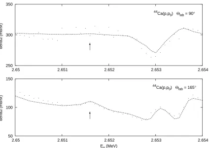
5.9 44Ca(p,p0) Data for Ep = 2.650–2.654 MeV . . . 54
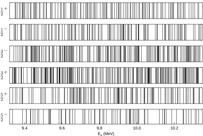
6.1 45Sc Observed Level Sequences . . . 59
6.2 Spacing Analysis for the s-wave Resonance Sequence – Previous Data . . . 61
6.3 Spacing Analysis for the p-wave Resonance Sequences – Previous Data . . . 62
6.4 Spacing Analysis for the d-wave Resonance Sequences – Previous Data . . . 63
6.5 Spacing Analysis for the s-wave Resonance Sequence . . . 64
6.6 Spacing Analysis for the p-wave Resonance Sequences . . . 65
6.7 Spacing Analysis for the d-wave Resonance Sequences . . . 66
6.8 Spacing Analysis for the f-wave Resonance Sequence . . . 67
6.9 The NNSD for the s-wave Resonance Sequence . . . 70
6.10 The NNSD for the p-wave Resonance Sequences . . . 71
6.11 The NNSD for the d-wave Resonance Sequences . . . 72
6.12 The NNSD for the f-wave Resonance Sequences . . . 73
6.13 P(0) Analysis for the s-wave Resonance Sequence . . . 74
6.14 The ∆3 Statistic for the s-wave Resonance Sequence . . . 76
6.15 The ∆3 Statistic for the p-wave Resonance Sequences . . . 77
6.16 The ∆3 Statistic for the d-wave Resonance Sequences . . . 78
6.17 The ∆3 Statistic for the f-wave Resonance Sequence . . . 79
6.18 γ2 and Pγ2 Plots for the s-wave Resonances . . . . 81
6.19 γ2 and Pγ2 Plots for the p-wave Resonances . . . . 82
6.20 γ2 and P γ2 Plots for the d-wave Resonances . . . . 84
6.21 γ2 and P γ2 Plots for the f-wave Resonances . . . . 85
6.22 Reduced Width Distribution for the s-wave Resonance Sequence . . . 87
6.24 Reduced Width Distribution for the d-wave Resonance Sequences . . . 89
6.25 Reduced Width Distribution for the f-wave Resonance Sequence . . . 90
6.26 J-Dependence of the Level Densities of 45Sc . . . 93
6.27 The Spin Cut-Off Parameter for45Sc . . . 94
6.28 The Parity Asymmetry in the 45Sc Level Densities . . . 95
A.1 The44Ca(p,p0) Cross-Section and Fits for Ep = 2.5–2.6 MeV. . . 100
A.2 The44Ca(p,p0) Cross-Section and Fits for Ep = 2.6–2.7 MeV. . . 101
A.3 The44Ca(p,p0) Cross-Section and Fits for Ep = 2.7–2.8 MeV. . . 102
A.4 The44Ca(p,p 0) Cross-Section and Fits for Ep = 2.8–2.9 MeV. . . 103
A.5 The44Ca(p,p 0) Cross-Section and Fits for Ep = 2.9–3.0 MeV. . . 104
A.6 The44Ca(p,p 0) Cross-Section and Fits for Ep = 3.0–3.1 MeV. . . 105
A.7 The44Ca(p,p 0) Cross-Section and Fits for Ep = 3.1–3.2 MeV. . . 106
A.8 The44Ca(p,p 0) Cross-Section and Fits for Ep = 3.2–3.3 MeV. . . 107
A.9 The44Ca(p,p0) Cross-Section and Fits for Ep = 3.3–3.4 MeV. . . 108
A.10 The44Ca(p,p0) Cross-Section and Fits for Ep = 3.4–3.5 MeV. . . 109
A.11 The44Ca(p,p0) Cross-Section and Fits for Ep = 3.50–3.53 MeV. . . 110
A.12 The44Ca(p,p1) Cross-Section and Fits for Ep = 2.5–2.6 MeV. . . 111
A.13 The44Ca(p,p1) Cross-Section and Fits for Ep = 2.6–2.7 MeV. . . 112
A.14 The44Ca(p,p1) Cross-Section and Fits for Ep = 2.7–2.8 MeV. . . 113
A.15 The44Ca(p,p1) Cross-Section and Fits for Ep = 2.8–2.9 MeV. . . 114
A.16 The44Ca(p,p1) Cross-Section and Fits for Ep = 2.9–3.0 MeV. . . 115
A.17 The44Ca(p,p 1) Cross-Section and Fits for Ep = 3.0–3.1 MeV. . . 116
A.18 The44Ca(p,p 1) Cross-Section and Fits for Ep = 3.1–3.2 MeV. . . 117
A.19 The44Ca(p,p 1) Cross-Section and Fits for Ep = 3.2–3.3 MeV. . . 118
A.20 The44Ca(p,p 1) Cross-Section and Fits for Ep = 3.3–3.4 MeV. . . 119
A.21 The44Ca(p,p 1) Cross-Section and Fits for Ep = 3.4–3.5 MeV. . . 120
onance Sequence . . . 205 D.2 N(E) Plots for Experimental and Unfolded Values ofEx for the p-wave
Res-onance Sequences . . . 206 D.3 N(E) Plots for Experimental and Unfolded Values ofEx for the d-wave
Res-onance Sequences . . . 207 D.4 N(E) Plots for Experimental and Unfolded Values ofEx for the f-wave
Res-onance Sequence . . . 208
Chapter 1
Introduction
Level densities have been investigated experimentally and theoretically for more than 50 years. The many practical applications of level densities have attracted interest from a variety of fields. Many experiments at the High Resolution Laboratory at the Triangle University Nuclear Laboratory have been performed over the last thirty years to determine the level densities of many different nuclei.
Level densities are usually determined by direct counting of observed nuclear states. Because experimental limitations have always produced imperfect data, even the best data may not allow precise determination of the level densities. However, recent research has produced improved analytic techniques that better determine the fraction of missing levels in a sequence. A better estimate of the completeness of a sequence will allow a more accurate determination of the level densities [Agv03b]. The application of these methods to several sets of data previously measured has produced improved results. However, the application to one data set resulted in results which have caused a reassessment of the quality of the previous data.
The p +44Ca reaction has been very well studied. The quality of the measurements made in these experiments was considered excellent. However, the application of the level density corrections to the 45Sc compound nucleus data has produced interesting results.
of the level densities [Agv03a]. The uncertainties in these level densities precluded definitive conclusions.
A by-product of the observed fraction corrections is an analysis method (the spac-ing anomaly analysis method) which provides a qualitative assessment of the purity and completeness of experimental sequences. By comparing the nearest-neighbor spacing dis-tribution, anomalous spacings which indicate potential misassigned or missing levels are revealed. This analysis indicated many specific suspected misassigned levels and many sus-pected general locations of unobserved resonances in the 45Sc data. The apparent parity dependence of the level densities in 45Sc can be questioned because of the large number of anomalies present in the data.
One goal of the present experiment was to investigate the specific resonances that the spacing anomaly analysis indicated were problematic. If the spacing anomalies can be removed, then the level densities will be better determined. Several factors have led to the conclusion that the experimental conditions have improved sufficiently to justify a re-investigation of the p +44Ca reactions. Recent experiments at the High Resolution Lab-oratory have shown that the beam resolution of the system has been improved. Passivated implanted planar silicon charged-particle detectors can measure the cross-sections of the in-elastic channels with greatly reduced background. Faster computers allow a more detailed analysis of the cross-section data. Thus weaker resonances should be observed, and more accurate Jπ assignments should be made. With higher quality resonance parameters, the level densities should be determined more accurately. With the level densities determined with reduced uncertainties, the observed parity dependence of the level densities can be evaluated more precisely.
The previous experiments that investigated the p + 44Ca reactions were performed
over a period of fifteen years [Wil75, Shr82, Shr83, Smi89] with vastly different experimental conditions and different methods of analysis. The different data sets are of uneven quality and reliability. The present experiment remeasured the 44Ca(p,p
0) and 44Ca(p,p1)
CHAPTER 1. INTRODUCTION 3
quality.
This experiment measured the differential cross-sections for the 44Ca(p,p0) and 44Ca(p,p
1) reactions for five angles over the energy range Ep = 2.50–3.53 MeV using 1.1– 1.5µg/cm2 thick44Ca targets. The experiment was performed using the modified KN-3000 Van de Graaff proton accelerator at the High Resolution Laboratory at the Triangle Uni-versity Nuclear Laboratory. Excellent results were obtained. The observed resonances were sorted into sequences which were tested statistically for completeness and purity. The level densities were determined with improved precision. The parity-dependence of the level den-sities with improved uncertainties was investigated, and the validity of the spacing anomaly analysis method was examined.
This work consists of seven chapters and four appendices. In the next chapter, an overview of the relevant parts of random matrix theory will be presented along with a discussion of two methods that estimate the observed fraction of levels in a sequence. Statistical tests of data quality are also described. Chapter 3 presents a brief description of the R-matrix theory used to analyze the cross-section data. Chapter 4 describes the experimental apparatus used to perform this experiment.
Chapter 5 describes the determination of resonance parameters and gives a com-parison of the resonances observed in this experiment with those from the previous work. Chapter 6 shows the results of several of the statistical analyses of the data. The nearest-neighbor spacing distributions and reduced width distributions are compared to theoretical predictions. The J-dependence and parity-dependence of the corrected level densities are investigated. Chapter 7 presents a summary of this experiment and the results.
Four appendices are included in this thesis. In Appendix A, the observed differential cross-section data and the theoretical fits for the 44Ca(p,p
0) and the 44Ca(p,p1) reactions
are presented. Appendix B lists the resonance parameters both in order of Ep and sorted by Jπ. Appendix C lists the adopted levels of45Ca used to identify analog resonances in 45Sc.
Statistical Analyses
The goal of the present experiment is to obtain pure and complete 45Sc level se-quences to measure accurately the level densities of 45Sc and to test the applicability of
the spacing analysis postulated by Agvaanluvsan [Agv02]. Agvaanluvsan analyzed the45Sc
level sequences measured by Smith [Smi89]. The analysis produced evidence of a possible parity dependence of the level densities [Agv03a]. However, this analysis also suggested a large number of possible quantum number misassignments and missing levels. This chapter describes the relevant theoretical issues for such an analysis. Section 2.1 describes random matrix theory (RMT) and several statistics used to analyze nuclear spectra. Section 2.2 dis-cusses the determination off, the fraction of states observed for an experimental sequence. Section 2.3 describes the spacing anomaly analysis and a new method to evaluate a mixed distribution of two GOE sequences.
2.1
Random Matrix Theory
CHAPTER 2. STATISTICAL ANALYSES 5
introduces an ensemble of random Hamiltonian matricesH which are real and symmetric. The nuclear Hamiltonian is treated as a random variable with a probability distribution P(H). To obtain the explicit form of the probability distribution, the distribution is as-sumed to be independent of the choice of basis vectors and the independent elements of H are assumed to be statistically independent. The explicit form ofP(H) can be shown to be
P(H) =e−atr(H2)+btr(H)+c (2.1)
wherea, b, andc are constants, and
tr(Hj) = N
X
k=1
λjk; (2.2)
here theλk are the eigenvalues of the nuclear Hamiltonian H. Each matrix H is assumed to describe equally probable interactions between particles. The GOE does not account for the dynamical properties of the nuclear Hamiltonian. However, statistical properties of nuclear level sequences can be investigated by examining the fluctuations about the averages of certain observables. The GOE makes parameter-free predictions about the fluctuation properties of nuclear spectra but says nothing about the dynamical properties.
2.1.1 Reduced Width Distribution
The probability distribution of the reduced widths (γ2) of a sequence of levels is
one test used to investigate the completeness of a nuclear sequence. A sequence of levels is defined as a set of levels all having the same quantum numbers (in this work, J and π). The GOE prediction for the distribution of the reduced widths of a sequence is called the Porter-Thomas distribution [Por56] and has the form
P(y) = √1
2πye
−y2. (2.3)
Herey= γλ2
is energy independent and requires a constant average reduced width. To describe this property globally, another quantity, the strength function S is used
S = hγ
2i
D (2.4)
whereDis the mean level spacing. Alternatively, the spreading width Γ↓ = 2πScan be used to describe the global characteristics of the reduced widths of a sequence. Since the mean level spacing changes exponentially with increasing energy, the characterization “global” may be questionable. However, hγ2i also effectively changes exponentially with increasing energy because the complexity of the eigenstates grows strongly with increasing energy [Guh98] such that these exponential dependencies cancel in Γ↓ and S. These parameters
are then suitable for describing the global properties of the reduced width distribution.
2.1.2 Nearest-Neighbor Spacing Distribution
The nearest-neighbor spacing distribution (NNSD) represents one of the key results of any of the ensembles of RMT. The NNSD provides information about the short-range order of the eigenvalues. The probability density function describes the probability of finding two adjacent levels with a spacings[Guh98]. It is convenient and conventional to work with the dimensionless variable x, defined as the ratio of the spacing between adjacent levels (s) and the average spacing between levels (D)
x= s
D. (2.5)
A system that follows the GOE statistics has a probability distribution approxi-mately of the form
PGOE(x) = π 2xe
−πx2
4 . (2.6)
CHAPTER 2. STATISTICAL ANALYSES 7
0 0.2 0.4 0.6 0.8 1
0 0.5 1 1.5 2 2.5 3
F(x)
x 0
0.2 0.4 0.6 0.8 1
0 0.5 1 1.5 2 2.5 3
P(x)
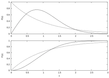
Figure 2.1: Nearest neighbor spacing distributions. The upper graph shows the probability function,P(x). The lower graph showsF(x), the integral ofP(x). The solid lines represent the GOE distribution and the dashed lines represent the Poisson distribution.
If a sequence contains a random set of uncorrelated energy levels with no special symmetries, the system will obey Poisson statistics. This distribution has the form
PP oisson(x) =e−x. (2.7)
This Poisson distribution has behavior quite different from the Wigner distribution atx= 0; the probability density function has its maximum atx = 0.
Histograms can in some cases be very sensitive to the choices of bins, and therefore the integral of the probability density function is also used to compare NNSD data with the predicted distributions. The integral of P(x) is defined as F(x), the definite integral over an intermediate variablex0 from zero tox,
F(x) =
Z x 0 P(x
Integrating Equations 2.7 and 2.6 gives:
FP oisson(x) = 1−e−x (2.9) FGOE(x) = 1−e−
πx2
4 (2.10)
Figure 2.1 illustrates the differences in P(x) and F(x) for the Poisson and GOE distribu-tions.
2.1.3 Dyson-Mehta ∆3 Statistic
The Dyson-Mehta ∆3 statistic [Dys63] was developed to investigate long-range
or-der. The Dyson-Mehta ∆3 statistic for a sequence of levels fromEmin toEmax is
∆3 = min
A,B
Ã
1 Emax−Emin
Z Emax
Emin
[N(E)−AE−B]2dE
!
, (2.11)
where the parameters A and B are parameters of the best straight line fit to the integral of the level density, N(E):
N(E) =
Z E 0
ρ(E)dE. (2.12)
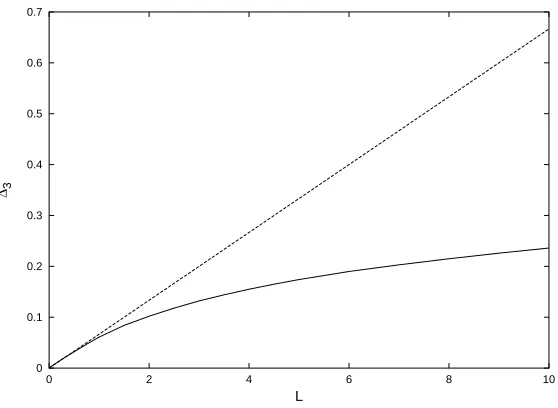
This statistic can be expressed as a function of L, the number of average spacings in an interval. For Poisson statistics
∆3poisson(L) =
L
15. (2.13)
For GOE statistics, ∆3must be evaluated numerically. For large values ofL, ∆3approaches
the value
∆3GOE ≈
1
π2(lnL−0.0687). (2.14)
Figure 2.2 illustrates ∆3 for Poisson and GOE distributions.
2.2
Missing Level Analysis
CHAPTER 2. STATISTICAL ANALYSES 9
0 0.1 0.2 0.3 0.4 0.5 0.6 0.7
0 2 4 6 8 10
∆3
L
Figure 2.2: The Dyson-Mehta ∆3 statistic is plotted as a function of L, the number of
average spacings. Theoretical predictions are shown for Poisson (dashed line) and GOE (solid line) distributions.
to the data to account for unobserved levels and to estimate the uncertainties introduced by the corrections. Two methods to estimate the number of missing levels in a sequence were described by Agvaanluvsanet al. [Agv02, Agv03b], a standard width analysis method and a new spacing analysis method. A brief description of both methods is presented here.
2.2.1 Width Analysis Method
The width analysis method uses the reduced widths, γ2, to estimate the observed
fraction of levels in a sequence. Some levels will remain unobserved due to the finite exper-imental threshold of observation. A perfect sequence (no missing or spurious levels) follows the Porter-Thomas distribution (Equation 2.3). An imperfect sequence can be described by a modified Porter-Thomas distribution which accounts for the distorted experimental distribution. This method includes only the effects of missing levels.
distribution,
Pf(y) =
0 : y < y0
1 erfcµqy0/2
¶ e −y/2 p
2πy : y ≥y0
. (2.15)
Applying the maximum likelihood technique to this distribution leads to the equation
hγ2i=hγ2iobs
³
1 +
r
2y0
π
e−y0/2 erfcp
y0/2 ´−1
. (2.16)
The solution to Equation 2.16 is obtained by calculating hγ12i from the experimentally obtained value ofhγobs2 i. The calculated value ofhγ12i is entered into the right-hand side of Equation 2.16 ashγobs2 iand a new valuehγ22iis computed. The process is repeated until the value entered into the right-hand side of Equation 2.16, hγn2−1i, and the calculated result
hγn2i converge. This final value ofhγn2i is then compared with the observed value, hγobs2 i, to obtain the observed fraction of levels in a sequence.
2.2.2 Spacing Analysis Method
The nearest-neighbor spacing distribution for a perfect GOE sequence follows the Wigner distribution. Experimental data are almost always incomplete. Unlike the reduced width distribution where widths are usually missed because they are too small to observe, the missing levels in the spacing analysis are randomly distributed. When levels are missing, the nearest-neighbor spacing distribution will not be described accurately by the Wigner distribution since some observed nearest neighbors are not actually nearest neighbors.
The distribution for the spacing of an imperfect sequence can be written as P(z) =
∞ X
k=0
akλp(k;λz). (2.17)
The parameter z is defined as z ≡ f x, where f is defined as f = Nobserved/Ntrue. The relative contributions of the k-th nearest-neighbor spacing distribution p(k;λz) are given by the parameters ak. The parameter λdescribes the incompleteness of the sequence.
CHAPTER 2. STATISTICAL ANALYSES 11
must also be normalized to one and have average values of k+ 1 when expressed in terms of the variablex. These conditions are expressed by the two constraints
∞ X
k=0
ak= 1, (2.18)
∞ X
k=0
ak(k+ 1) =λ. (2.19)
The parametersak can be determined by defining an entropy
S{ak}=−
∞ X
k=0
aklnak (2.20)
along with two Lagrange multipliers α and β for the two constraints (Equation 2.18 and Equation 2.19). Maximizing the entropy requires
δ
( −
∞ X
k=0
aklnak−α
∞ X
k=0
ak−β
∞ X
k=0
(k+ 1)ak
)
= 0. (2.21)
The values that maximize the entropy areak=f(1−f)k and λ= 1/f. These values yield the expression
P(x) =
∞ X
k=0
f(1−f)kP(k;x). (2.22)
The maximum likelihood method is then applied to Equation 2.22 which generates a value of f and a value for the uncertainty inf for a sequence. The two methods, spacing and width, complement each other and provide independent tests of the missing fraction of levels in a sequence.
2.3
Spacing Anomaly Analysis
not indicate specific regions where the missing levels are likely to be found. Section 2.3.1 describes a method that uses the nearest-neighbor spacing distributions to locate suspected spacing anomalies, and Section 2.3.2 explains a new method that uses the value of the nearest-neighbor spacing distribution atx= 0 to estimate the number of spurious levels in a sequence.
2.3.1 Spacing Anomalies
The nearest-neighbor spacing distributions for nuclear level sequences are expected to follow the Wigner distribution (Equation 2.6). Observed nearest-neighbor spacing distri-butions for level sequences can be expressed in terms of the variable x≡ Ds and compared directly to the Wigner distribution. As shown in Section 2.2.2, this comparison to observed data gives an indication of the percentage of missing levels. However, the locations of the missing levels are unknown.
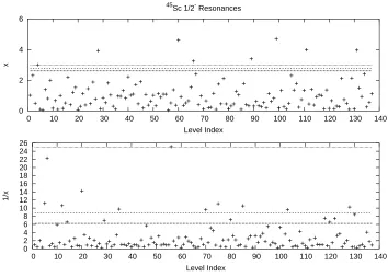
An anomalous spacing is defined as a nearest-neighbor spacing that has a value ofx that is either so small or so large as to be very unlikely given the Wigner distribution. Large values ofxsuggest a missing (unobserved) level. Listed in Table 2.1 are the values ofxfor a given confidence level. Sufficiently large spacings strongly suggest missing levels. However, experimental evidence may be very difficult to obtain, since the resonance probably would have already been observed if it were easy to detect. Some of the missing resonances will be observed in the current experiment, but some will remain unobserved due to the finite experimental threshold. Also, there is only limited information regarding the locations of suspected missing levels. The energy interval suggested by a large spacing anomaly can be large and may contain many other resonances with different quantum numbers. Thus, correcting all large spacing anomalies with the current experimental methods is unlikely.
CHAPTER 2. STATISTICAL ANALYSES 13
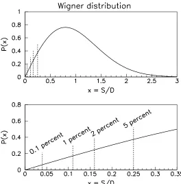
Table 2.1: Percentage of levels with spacings ≥x. x= Ds % of levels≥x
1.95 5 %
2.23 2 %
2.42 1 %
3.00 0.1 %
is considered. Table 2.2 lists the values of 1/x for a given confidence level. Small spacing anomalies can be more easily investigated since the locations of both levels are already known. Studying the pair of resonances that produced the small spacing with improved resolution and determining the resonance parameters of these resonances with improved confidence may produce a quantum number reassignment and eliminate the small spacing anomaly. Thus, a small spacing anomaly should be easier to correct experimentally than a large spacing anomaly, because the levels that produce a small spacing anomaly have always been previously observed.
Table 2.2: Percentage of levels with spacings≥1/x. x= Ds 1/x % of levels≥1/x
0.25 4.00 5 %
0.16 6.25 2 %
0.11 8.84 1 %
0.04 25.00 0.1 %
Figure 2.3: The relative probability of small spacings for a Wigner distribution. The upper graph shows the Wigner distribution. The dashed lines indicate the values of x for which the probability of finding a value smaller than that value of x are 0.1%, 1%, 2%, and 5%. The lower graph shows the small-xportion of the upper graph in greater detail.
number.
CHAPTER 2. STATISTICAL ANALYSES 15
0 2 4 6 8 10 12 14 16 18 20 22 24 26
0 10 20 30 40 50 60 70 80 90 100 110 120 130 140
1/x
Level Index 0
2 4 6
0 10 20 30 40 50 60 70 80 90 100 110 120 130 140
x
Level Index
45
Sc 1/2- Resonances
Figure 2.4: x and 1/x plots for the Jπ = 12− sequence before the current measurements. The dashed lines represent the 2%, 1% and 0.1% confidence level.
2.3.2 P(0) Analysis
One flaw of the spacing anomaly analysis described in Section 2.3.1 is that only levels with extreme spacings will be indicated by plottingxand 1/x. The method does not identify misassignments or missing levels if the nearest-neighbor spacings are not anomalously large or small. A method that does not depend on spacing anomalies to quantify the purity of a sequence has been considered.
complicated, it reduces to a very simple form atx= 0:
P(0) = 1− n
X
i
fi2, (2.23)
with fi being the relative probability of the mixed sequences. For proton resonance data, the ambiguity in the fitting analysis reduces to mixing only two sequences, i.e.,n= 2. P(0) can then be written
P(0) = 1−f12−f22. (2.24)
Since f1+f2= 1, Equation 2.24 reduces to a quadratic of the form:
f12−f1+P(0)
2 = 0. (2.25)
Chapter 3
Reaction Formalism
The most useful formalism for describing compound nuclear resonances is the R-matrix theory, formulated by Wigner and Eisenbud [Wig46b, Wig46a, Wig47]. R-matrix theory has been used very successfully to describe the charged-particle scattering cross-sections measured at the High Resolution Laboratory. Section 3.1 contains a brief description of R-matrix theory as formulated by Lane and Thomas [Lan58] and presented in many theses [Wil73, Wat80, Nel83, Smi89]. Section 3.2 describes isobaric analog resonances (IAR).
3.1
R-Matrix Formalism
R-matrix theory makes several assumptions. R-matrix theory only describes non-relativistic quantum mechanical systems. Three-body systems are not allowed unless con-sidered as a succession of two-body reactions. Only reactions in which the initial and final states consist of two particles are considered in this description of R-matrix theory. There must be a distance beyond which the interaction between the two particles ceases. This distance is called the “channel radius”.
and44Ca(p,p1) reactions, and thus the two-body requirement is met. Finally, since nuclear
forces are short range, a “channel radius” ac can be defined.
R-matrix theory can be formulated in different representations. When used to de-scribe the interaction of an unpolarized beam and target, the channel spin representation is normally used. The spin of the target and the spin of the projectile are coupled to form a channel spin, which is then coupled with the relative angular momentum of the target and projectile to form the spin of the compound state. This method is used since the cross-sections are incoherent in channel spin, and the total cross-section can be expressed as a weighted sum of the cross-sections for each channel spin. The compound nucleus is cre-ated via an “entrance” channel which consists of the projectile and target. The compound nucleus then decays through an “exit” channel. Channels which are not allowed by some conservation law are called “closed” while allowed channels are called “open”.
A pair of interacting nuclei is labelled by the letter α which specifies the quantum states of each nucleus in the pair. The two nuclei have spins, I1 and I2, which are
vector-coupled to form the channel spins. The resultant channel spin can assume values between
| I1−I2 | and | I1+I2 |. The two nuclear spins also have corresponding projections i1
and i2, and the channel spin has a projectionν. The relative orbital angular momentum `
and its projectionmare also specified for the pairα. The channel spin, s, and the relative angular momentum, `, are combined to give a resultant total angular momentum,J (with projection M). A channel c for the pair α is then defined by the angular momentum coupling {α(I1, I2)s`JM}. For variables that do not depend on angular momentum, we
can use either the channel label c or the pair label α without confusion. However, some variables will refer only to a specific channel, and for those we must maintain the channel label. In what follows, every effort is made to indicate this distinction.
CHAPTER 3. REACTION FORMALISM 19
definitions are:
the reduced mass of the system Mc =Mα =
Mα1Mα2 Mα1+Mα2
,
the wave number kc =kα=
·2MαEα
¯ h2
¸12
,
the relative velocity vc =vα = ¯ hkc Mc ,
the Coulomb field parameter ηc =ηα=
Zα1Zα2e2 ¯ hvα
,
and a dimensionless parameter ρc =ρα=kcrc.
To solve the Schroedinger equation, the radial space is separated into an external region (rc > ac) and internal region (rc < ac). Only the Coulomb force is present in the external region, and the Schroedinger equation can be solved exactly. The resulting external wave functions are
ψextc = χc(rc√)uα`(rc) vc
, (3.1)
where
χc(rc) =
"
i`Ym
` (θα, φα) rc
#
ψαsν (3.2)
are the surface wave functions which are mutually orthogonal and normalized at rc = ac. The Ym
` are the usual spherical harmonics, and ψαsν are the channel spin wave functions formed by the vector coupling of the spin wave functions of the two interacting nuclei. The functionuα` is the radial wave function which satisfies the following:
d2u
α` dr2 c + ·2M α ¯ h2 ¸
[Ec−Vc]uα`(rc) = 0. (3.3)
The potential Vc includes both the Coulomb and “centrifugal” potential energies and has the form:
Vc=
Zα1Zα2e2 r2
c
+¯h
2`(`+ 1)
2Mcrc2
. (3.4)
the regular and irregular Coulomb functions [Jah60]. The general solutions of the radial wave function are linear combinations of the regular and irregular Coulomb functions and represent incoming and outgoing waves:
Ic+= [Gc−Fc]eiωc (3.5)
and
O+c = [Gc+Fc]e−iωc. (3.6)
The parameter ωc takes the form:
ωc=ωα` = `
X
n=1
tan−1
µηα
n
(3.7)
The complete channel wave functions which represent incoming and outgoing waves of unit flux in the external region are then
Ic =
χc(rc)Ic+
√v
c
(3.8)
and
Oc = χc(rc)O
+
c
√v
c
. (3.9)
A collision matrixUcc0 can be introduced in the general solution of the wave function
in the external region. The general solution can be expressed as a linear combination of Ic andOc. The solution chosen represents the external wave function for a particular incoming wave and has the form
ψcext=Ic−
X
c0
Ucc0Oc0. (3.10)
The collision matrix is the amplitude of the outgoing wave in channelc0 which is associated with a particular incoming wave in channel c. One example would be elastic scattering which is described by Equation 3.10 when c = c0. All the information necessary to solve
CHAPTER 3. REACTION FORMALISM 21
Several methods have been considered to obtain Ucc0. One method would be to
assume a nuclear potential in the internal region. With a nuclear potential, the Schroedinger equation could be solved to generate a wave function for the internal region which could then be matched to the external wave function at the nuclear surface (rc = ac). However, the results of this method would rely on the parameters chosen to describe the nuclear potential. The R-matrix theory instead proposes a complete set of states which are eigenstates of the Hamiltonian in the internal region. This postulate covers all possible resonances of the compound nuclear system and has the form
Hλψλ=Eλψλ (3.11)
with
Z
ψ∗λψλ0dr=δλλ0. (3.12)
The channel wave functions can then be expressed in terms of the overlap of the internalλ states with the appropriate surface wave functionsχc. Integrating over the nuclear surface of radius ac gives
χλ(rc) =
Z
ac
χ∗cψλdS, (3.13)
which are eigenfunctions with eigenenergiesEλin channelcand have arbitrary, real, energy-independent boundary conditions
·
ρcχ
0
c χc
¸
rc=ac
=Bc. (3.14)
Here the prime indicates differentiation with respect toρc.
The wave functions in the internal region for any energy E can be expressed in terms of an expansion of the eigenfunctions χλ(rc). The coefficients of the expansion can be determined by applying Green’s theorem. The resulting internal wave function can be written as
ψcint(rc) =Rcc0 "
acdψ int c (rc)
dr −Bcψ int c (rc)
#
rc=ac
where the Green’s function,Rcc0, that relates the value of the wave function in the internal
region to its derivative on the surface is Rcc0 =
X
λ
γλcγλc0
Eλ−E
. (3.16)
The reduced widths, γλc, take the form
γλc=
"
¯ h2 2Mcac
#12
χλ(ac) =
"
¯ h2 2Mcac
#12 Z
ac
χ∗cψλdS. (3.17) Equations 3.16 and 3.17 define the elements of the R-matrix and the reduced widths. The collision matrix (U-matrix) may be expressed in terms of the R-matrix by equating the logarithmic derivatives of the internal and external wave functions at rc =ac. The result can be shown to be
Ucc0 =ei(ωc+ωc0−φc−φc0) ·
δcc0 + 2iP
1 2
c 1
1−Rcc0Lc0Rcc 0P 1 2 c0 ¸ (3.18) where Lc = · ρcO 0 c Oc ¸
rc=ac
−Bc =hScλ−Bci+iPc. (3.19) Pc is called the penetrability; it is proportional to the transmission probability through the external barrier and can be expressed as
Pc=
· ρ
c F2
c +G2c
¸
rc=ac
. (3.20)
Sc is the shift function and has the form Sc =
·
ρc
FcFc0+GcG0c F2
c +G2c
¸
rc=ac
. (3.21)
The quantityφc is called the hard-sphere phase shift and has the form φc = tan−1
µF
c Gc
. (3.22)
The quantityωc is the Coulomb phase shift for channelc.
A quantity that represents the total energy shift from the eigenenergyEλand results from a mismatch of the external and internal boundary conditions is
∆λ=−
X
c0 h
Sλc0−Bc0 i
CHAPTER 3. REACTION FORMALISM 23
The total laboratory width for a level is
Γλ=
X
c
Γλc, (3.24)
where the partial laboratory width for a channel,
Γλc= 2Pcγλc2 , (3.25)
is the transition probability from the stateλvia the channelc. The partial laboratory width contains a factor from both the external region (penetrability) and internal region (reduced width). The penetrability is a measure of the kinematic effects in the external region. The penetrability decreases as` increases. Thus high`states will generally have smaller values of laboratory partial widths than low`states. The reduced widths have the external region effect removed which allows for a comparison of the strength of the nuclear coupling to the entrance channel.
The R-matrix and collision matrix are both diagonal in total spin and in parity. The cross-section includes contributions from all spins and parities. The relationship between the differential cross-section and collision matrix is derived by Lane and Thomas and is programmed in the FORTRAN code MULTI6. The equation is
dσαs,α0s0
dΩα0 =
π k2
α|
Cα0(θα0)|2δα0s0,αs
+ 1
k2
α(2s+ 1)
X
L
BL(α0s0, αs)PL(cosθα0) (3.26)
+ π
1 2 k2
α(2s+ 1)
X
J`
(2J+ 1)δα0s0`0,αs`Re h
iTαJ0s0`0,αs` i
Cα0(θα0)P`(cosθ),
where
BL(α0s0, αs) = 1 4(−1)
(s−s0) X
J1J2`1`2`0
1`02
Z(`1J1`2J2, sL)
× Z(`01J1`02J2, s0L) ³
TαJ10s0`0
1,αs`1
´ ³
TαJ20s0`0
2,αs`2
´∗
, (3.27)
and
Cα = 1 [4π]12
ηαcsc2
µθ
α 2
e−2iηαlog[sin(θα2 )]. (3.29)
TheZ coefficients are theZ coefficients of Biedenharnet al. [Bie52] with the phase conven-tion of Huby [Hub54]. TheP`(cosθ) are the Legendre polynomials with the phase convention of Condon and Shortley [Con51].
The first term in Equation 3.26 represents pure Coulomb scattering, the second term represents resonance scattering and reaction, and the third term represents the interference between the first two terms. The Coulomb and interference terms vanish except for elastic scattering. To obtain the experimentally measured cross-sections for unpolarized beam and target, Equation 3.26 must be summed over s0 and averaged over s. The summing and
averaging is also performed by MULTI6; the result is dσα,α0
dΩα0
= 1
(2I1+ 1)(2I2+ 1) X
ss0
dσαs,α0s0
dΩα0
. (3.30)
3.2
Isobaric Analog Resonances
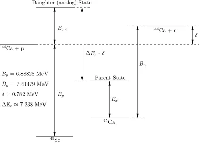
Isobaric analog states are defined as nuclear states that are multiplets of a given isospin, T. These nuclei differ by the exchange of a neutron for a proton. In an analog parent-daughter system, both nuclei have A nucleons, but the parent-daughter has one more proton and one less neutron than the parent. If the nuclear force is charge independent and charge symmetric, then the isospin quantum number T = N−2Z is a good quantum number, and the energy difference between parent and daughter is ∆Ec−δ, where ∆Ec is the Coulomb energy difference andδ is the proton-neutron mass difference. Corresponding states in the parent and daughter have the same values of Jπ. The energy differences between parent and daughter are illustrated in Figure 3.1.
From Figure 3.1, an the excitation energy of the parent (Ex) and the center of mass proton energy (Ecm) are related by
CHAPTER 3. REACTION FORMALISM 25
where Bn is the binding energy of the last neutron in the parent nucleus, and Bp is the binding energy of the last proton in the daughter nucleus. Analog resonances were used to determine values of ∆Ec. J¨anecke has determined a semi-empirical approximation for ∆Ec given by [J¨an69]
∆Ec =
C1Z<+C2
A13
, (3.32)
where A is the mass of the parent system, Z< is the proton number of the target and C1
and C2 are constants. For theA = 45 system,Bn = 7.41479 MeV,Bp = 6.8882 MeV, and J¨anecke’s estimate gives ∆Ec = 7.238 MeV. Therefore, the approximate relation between Ecm for p + 44Ca resonances and Ex in 45Ca is Ecm = Ex - 0.177 MeV. ∆Ec can vary significantly; thus the uncertainty in this calculation can be large.
44Ca + p
Daughter (analog) State
45Sc
45Ca
Bp = 6.88828 MeV Bn = 7.41479 MeV δ = 0.782 MeV ∆Ec ≈7.238 MeV
Parent State
Bp Ecm
∆Ec - δ
Ex
Bn
44Ca + n
δ
Figure 3.1: Analog state energy schematic for the 45Ca and 45Sc system. B
Chapter 4
Experimental Setup
The data for this experiment were collected at the High Resolution Laboratory (HRL) of the Triangle Universities Nuclear Laboratory (TUNL). The HRL is shown schemat-ically in Figure 4.1. The main component of the HRL is a modified KN-3000 Van de Graaff positive ion accelerator. Recent experiments have produced tunable proton beams over the energy range 0.9–4.0 MeV. Combined with the laboratory’s unique electrostatic ana-lyzer (ESA), this accelerator produces a proton beam with excellent beam energy resolution (200–300 eV) which allows the investigation of weak, closely spaced nuclear resonances. The accelerator and ESA will be discussed in Section 4.1. The detectors and the data acquisition system will be explained in Section 4.2. The experimental procedure will be outlined in Section 4.3 and the target fabrication described in Section 4.4.
4.1
Accelerator
KN 3000 Van de Graaff
Electrostatic Analyzer Analyzing
Magnet
(p,p) Chamber
(p,γ) Chamber
Figure 4.1: Floorplan of the High Resolution Laboratory at TUNL (not to scale). The (p,p) chamber was used in this experiment.
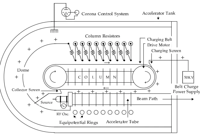
combination of dry CO2 and N2 for electrical insulation. Along this column runs a 190-inch
vulcanized rubber belt which carries positive charge to the dome. Beside the column is a stainless steel accelerator tube rated for potentials as high as four million volts. Some of the charge deposited on the dome flows through a series of column-mounted 600-MΩ resistors, resulting in a series of equipotential planes which produce constant acceleration over the length of the tube. To maintain constant charge on the dome, a set of corona needles are mounted on the inside of the tank between the dome and the tank wall. Current flows from the dome through the needles, which allows the amount of positive charge on the dome to be altered. The corona controller is partially driven by a capacitive pickoff signal (CPO). The CPO is an electrically isolated metal plate which monitors the AC components of the dome voltage. The CPO generates a signal which is used as feedback to reduce low frequency AC fluctuations (20 Hz or less).
During normal operation, two ion beams are produced by a radio frequency (RF) ion source, which sits at the unsupported end of the cantilevered column. High purity H2
gas is leaked into a glass source bottle. An RF field applied to this bottle results in the gas becoming a plasma. The disassociation of the H2 results in protons (H+) and singly
CHAPTER 4. EXPERIMENTAL SETUP 29
Figure 4.2: Schematic of the modified KN-3000 Van de Graaff accelerator.
two species are deflected by different amounts due to the difference in their charge-to-mass ratios. The magnet is set so that the H+ beam is deflected by 25◦ into a beam line that terminates at the target chambers and the H+2 beam is deflected 17◦ into the ESA to be used for diagnostic purposes.
The ESA is basically a pair of curved metal plates. This system is designed to monitor and correct the energy fluctuations of the accelerated proton beam. The plates are separated by 4.57 mm and form a 90◦ arc. The plates are biased to voltages of equal
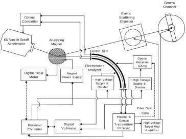
magnitude but opposite polarities such that the H+2 beam can only pass through the ESA if it is within a certain energy tolerance. The total voltage difference between the plates is set to the desired proton beam energy divided by 111.37. The voltage settings are monitored by a high precision voltmeter and a control PC to ensure that the proper voltage is maintained. There are also two sets of lateral slits, the corona slits at the entrance and the image slits at the exit of the ESA. Figure 4.3 shows the various feedback loops used by the ESA.
KN Van de Graaff Accelerator Corona Controller Digital Tesla Meter Magnet Power Supply Analyzing Magnet Digital Voltmeter Personal Computer Electrostatic Analyzer
- High Voltage Supply &
Divider
+ High Voltage Supply & Divider Optical Receiver &Amp High Voltage Target Rod Amplifier Fiber Optic Cable Preamp & Optical T r a n s m i t t e r /
Receiver Elastic Scattering Chamber Gamma Chamber
CPO Control Slits
Figure 4.3: High Resolution Laboratory Control Loops. A current difference signal from the corona control slits is used to regulate voltage on the terminal. A current difference signal from the image slits located at the end of the ESA is used to regulate the magnetic field, the potential on the outer plate, and to adjust the target rod voltage.
terminal voltage. A slit difference signal is measured by sampling the difference in the H+2 beam current on the left and right corona slits. This signal is a direct indication of the slow energy fluctuations inherent in a belt-driven accelerator. The corona controller attempts to minimize this slit difference signal in order to maintain a mono-energetic proton beam. Used in conjunction with the CPO feedback, this system dramatically decreases the amplitude of the dome voltage fluctuations (to a value ≈1 kVp−p). The corona slits are also used in the automated creation of yield curves which will be discussed shortly.
CHAPTER 4. EXPERIMENTAL SETUP 31
PC adjusts the magnet setting to minimize the slit difference signal. This increases the stability of the beam and is crucial when automating the generation of yield curves. The slit difference signal is also applied to the outer plate of the ESA which slightly alters the voltage difference between the ESA plates. This is done to increase the H+2 beam stability by accounting for the small fluctuations in beam energy measured by the slit difference signal. Finally, the slit difference signal is sent to the target rod driver. The target rod is normally biased at 3 kV; the slit difference signal is amplified by the target rod driver and added to the bias voltage. In this manner, the proton beam energy is corrected for dome voltage fluctuations as it approaches the target. The result of these control loops is to create a nearly mono-energetic beam with outstanding resolution and reduced energy drift. The control loops are also used for the critical function of automating the generation of yield curves. This is accomplished by the TUNL XSYS data acquisition software system, which can change the energy of the proton beam automatically. First the VAX and control PC change the voltage of the ESA to the voltage that corresponds to the new proton beam energy. Because the molecular beam will no longer be properly centered in the ESA, the image slit difference will increase. The control PC will then adjust the analyzing magnet to minimize the image slit difference signal. As this is accomplished, the H+2 beam will now generate a slit difference signal at the corona slits. The corona driver will alter the dome voltage to minimize this signal, and the proton beam will now be at a new energy without any operator involvement. This process is monitored by the control PC to inhibit data acquisition if problems arise.
4.2
Detectors and Data Acquisition System
located just in front of the target chamber. The 44Ca targets are mounted on a target rod which holds four targets and a tuning ring. The beam current is measured with a Faraday cup at the rear of the target chamber. For this experiment, a typical beam was 6-8µA with less than 5 nA on the tuning ring and last collimator.
90 108 135 165
150
Beam Collimator
Target
Vacuum
Faraday cup Port
Assembly
Viewing Ports
Figure 4.4: High Resolution Laboratory charged particle target chamber. The beam is collimated before striking the target, which is set at 330◦. The beam is measured at the
Faraday cup. This chamber was designed by Westerfeldt [Wes82, Wes83].
Mounted inside the target chamber were five passivated implanted planar silicon (PIPS) detectors manufactured by Canberra. The PIPS detectors were the partially de-pleted (PD50-13-300AM) model with 50 mm2 active area and 300 micron depth. The de-tectors are factory tested to have a resolution of ≤13 keV (FWHM) for 241Am-5.486 MeV alpha particles. Each detector was mounted on its own stand in the horizontal plane of the target and with a collimator in front of the detector. Dipole magnets were placed on the collimator snouts to reduce noise from electrons attracted to the positively biased detector. The detectors were located such that the count rates for all five detectors were approximately equal. The detector solid angles are listed in Table 4.1.
CHAPTER 4. EXPERIMENTAL SETUP 33
Table 4.1: Detector solid angles for the five detectors used in this experiment. Solid angles were chosen such that there were approximately equal count rates in each detector.
Detector Ω Angle (msr)
90◦ 0.53 108◦ 0.90
135◦ 1.54 150◦ 1.84 165◦ 2.04
then amplified by a linear amplifier (Ortec 572) which outputs both a bipolar (timing) and unipolar (energy) signal. Both outputs are used to process the signal. The unipolar singal is digitized and displayed in a spectrum via the VAX unless prevented by the bipolar signal discrimination process, which is used to eliminate carbon scattering events and to reduce electronic dead time.
4. EXPERIMENT AL SETUP 34 4 Faraday Cup Manual & Beam Limit Data On/Off Digital Current Meter PC Data On/Off Crate Inhibit &
Alarm CAMAC Crate
CAMAC Crate Terminator Preset Scaler
Buffer
Inhibit Out
Hex Scaler (2) Router Decoder ADC/Buffer Interface Scaler Interface (2) Router Encoder Multiplexer Multiplexer Gate Box ADC system busy Delay Line Linear Amplifier Timing SCA Gated SCA Delay
CHAPTER 4. EXPERIMENTAL SETUP 35
The SCA also serves as a discriminator to eliminate low and high energy noise by setting upper and lower limits on the signals. When an event is to be processed, the gated SCA also sends a signal to a Gate and Delay Generator (Ortec 416A). This creates a signal which is sent directly to the scalar interface to count the number of acceptable events. Thus, the signals that are determined acceptable exclude carbon scattering events and events with too low or too high an amplitude.
The unipolar signal is sent directly to the multiplexer after a 900-ns delay, which corresponds to the processing time of the bipolar signal. When the multiplexer is given the command to accept a signal, it also generates a routing signal which indicates the detector from which the digitized signal came. This signal is decoded and sent to the buffer interface, where the digitized signal is tagged to maintain the detector identification. This information accumulates in the buffer in the CAMAC crate to await transfer to the Microprogrammable Branch Driver (MBD) and then to the VAX. A final piece of information waits in the CAMAC crate as well. The Gate and Delay Generator signal is sent to the scalar interface and then to a hex scalar. The number of signals sent to the hex scalar for each detector is compared to the number of digitized events to calculate the dead time for each detector. Typical dead times for this experiment were between 3–10%.
Finally, there is a series of inhibits to prevent data from accumulating during un-acceptable conditions. Such conditions include the target rod being unbiased, large fluctu-ations of the beam currents, or the ESA voltage being outside acceptable limits. The last is the most important as it prevents data accumulation when the proton beam energy is fluctuating abnormally or while energy steps are being performed.
The data collected are stored in 512-channel spectra. The TUNL XSYS data acqui-sition softare allows data acquiacqui-sition until a preset amount of charge has been accumulated. A typical spectrum is shown in Figure 4.6 with the peaks of interest corresponding to
44Ca(p,p
0),44Ca(p,p1), and 44Ca(p,p2). The16O(p,p0) peak is identified and used for
0 2000 4000 6000 8000 10000
0 100 200 300 400 500
Counts
Channel Number 44Ca(p,p
0) 16O(p,p0)
44Ca(p,p1) 44Ca(p,p2)
Figure 4.6: Charged particle spectrum for Ep = 3.0938 MeV. The 44Ca(p,p) peaks were gated and summed to produce yield curves. Note the flat area near channel 200 where the
12C(p,p
0) peak has been removed electronically.
and stored as a function of energy. The system automatically increments the energy on reaching the preset amount of charge and begins a new set of spectra. For this experiment, the preset charge was generally 400 or 500µC, which required run times of 90–180 seconds. The preset value was chosen to provide acceptable statistics (∼ 1%) for the 44Ca(p,p
0)
reaction.
4.3
Experimental Procedure
CHAPTER 4. EXPERIMENTAL SETUP 37
VAX using a set of interactive command codes. Before the automated generation of yield curves begins, the spectra must be energy calibrated. Calibration is accomplished by iden-tifying the peaks in the spectra — usually 44Ca(p,p0), 44Ca(p,p1), and 16O(p,p0) — and
determining the energy of the scattered protons from kinematic considerations. With this information, the VAX can track the peaks of interest as they change with bombarding energy.
When the calibrations are complete and the electronics properly set, the starting energy, energy step size, and total amount of charge to be collected per point are entered into the VAX. For this experiment, data were collected over the energy range 2.5–3.5 MeV in 100-eV energy steps. As noted above, the total charge collected per point was 400 or 500 µC. The VAX will collect data until the preset amount of charge is reached, sum the data for the on-line yield curves, and increment the energy to continue the experiment. Data collection continues until manually halted. Halting occurs when experimental conditions deteriorate for such reasons as target degradation, erratic beam fluctuations, or equipment failure. The data is thus taken in segments. To ensure sufficient overlap between segments for identification and energy calibration purposes, the energy is stepped back a sufficient amount to provide an overlap in the two neighboring segments. This experiment was taken in many segments (∼30) over two one-week periods.
40 60 80 100 120 140 160
2.5 2.51 2.52 2.53 2.54 2.55
d
σ
/d
Ω
(mb/sr)
Ep (MeV)
44
Ca(p,p0) Θlab = 165°
Figure 4.7: 44Ca(p,p0) yield curve over the energy range Ep = 2.50-2.55 MeV.
4.4
Targets
Two types of targets were used for this study,44Ca and56Fe. The44Ca targets were used for the collection of new data, while the56Fe targets were used to provide an absolute
beam energy calibration [Nel83]. Both targets were thin films evaporated onto carbon foils. For44Ca the target thickness was 1.1–1.5µg/cm2, which corresponds to 70–120 eV average
energy loss. This is well below the machine energy resolution. The 56Fe targets did not
have to be as thin, since they were only used for energy calibration. The thickness for the iron targets was ∼2.5µg/cm2, which corresponded to∼200 eV energy loss.
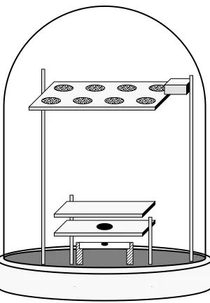
CHAPTER 4. EXPERIMENTAL SETUP 39
current flowing between the electrodes. There was also a shutter and aperture to allow the boats to be heated without deposition on the targets. Clean glass slides were placed on top of the target rings in the frame to prevent the target material from depositing on the back of the targets.
For 44Ca target fabrication, a 0.01” closed tantalum boat was used. The calcium was in the form of CaCO3 enhanced to 95.9% 44Ca. To reduce the carbonate and obtain
calcium targets, tantalum powder was added at a 1:6 calcium carbonate to tantalum ratio to provide sufficient reducing agent. This mixture is then inserted into the closed boat and placed inside the bell jar. The current was slowly raised using the high current electrodes to∼70 A at which point reduction occurs. Reduction was indicated by rapidly increasing pressure inside the bell jar and typically lasted for 5 minutes. After reduction, the current was raised to ∼ 150 A and evaporation occurred. The deposition was monitored via a quartz crystal thickness monitor and calibrated using Coulomb scattering measurements. The proper thickness was easier to achieve when the evaporation process was performed slowly. To produce a batch of targets, the evaporation process lasted∼15 minutes.
For56Fe target fabrication, a 0.005” open tungsten boat was used. Each evaporation used 0.02 g of Fe2O3 enriched to 99.87% 56Fe. The boat and isotope were placed into the
evaporation chamber, sealed with a miniature bell jar, and evacuated. After the jar was evacuated (≤ 1 µTorr), the system was filled to ∼ 300 Torr with hydrogen gas. The hydrogen was used as a reducing agent. The current was raised to ∼100 A; reduction was characterized by the red powder form of Fe2O3 turning black and melting onto the boat.
Chapter 5
Determination of Resonance
Parameters
The 44Ca(p,p
0) and 44Ca(p,p1) differential cross-sections were measured at five
an-gles, Θlab = 90◦, 108◦, 135◦, 150◦, and 165◦, over the energy range Ep = 2.500–3.534 MeV in 100-eV steps. 44Ca targets were prepared with a thickness of 1.1–1.5µg/cm2. Resonance parameters were determined for 809 resonances. Figure 5.1 shows the cross-sections and fits for several angles and reactions. This chapter describes the identification and assignments of the observed resonances. Section 5.1 explains both the FORTRAN code MULTI6 which was used to fit the data and the angular momentum coupling scheme used in the fitting pro-cedure. Section 5.2 discusses the energy calibration. Section 5.3 provides specific examples of the fitting procedure, and Section 5.4 presents the results of the differential cross-section analysis.
5.1
MULTI6
0 5 10 15 20 25
2.5 2.6 2.7 2.8 2.9 3 3.1 3.2 3.3 3.4 3.5 Ep (MeV)
44
Ca(p,p1) Θlab = 165°
0 50 100 150 200 250
2.5 2.6 2.7 2.8 2.9 3 3.1 3.2 3.3 3.4 3.5
d
σ
/d
Ω
(mb/sr)
44
Ca(p,p0) Θlab = 165°
0 100 200 300 400
2.5 2.6 2.7 2.8 2.9 3 3.1 3.2 3.3 3.4 3.5
44
Ca(p,p0) Θlab = 90°
Figure 5.1: Cross-sections and fits for 44Ca(p,p0) and 44Ca(p,p1) at Θlab = 165◦ and
44Ca(p,p
0) at Θlab = 90◦.
cross sections. MULTI6 calculates theoretical cross-sections based on many input parame-ters and can calculate simultaneously the differential cross-sections for both reactions at all five observed angles. The calculated cross-sections are visually compared to the normalized experimental sections. Input parameters are adjusted until the experimental cross-sections and calculated cross-cross-sections compare well. Typically, many executions of MULTI6 are necessary for each observed resonance.
CHAPTER 5. DETERMINATION OF RESONANCE PARAMETERS 43
44Ca
Ground State
44Ca
Ground State Compound State
1st Excited State 2nd Excited State
45Sc
Jπ
0+ 0+
0+
2+ Entrance
Channel: `, s
(p,p0)
(p,p1) (p,p2)
J =`⊕s
π= (-1)` s = 0⊕ 12 =
1 2
s0 = 2
⊕12 = 3
2,
5 2 s00 = 0
⊕ 12 = 1 2
`= 0, 1, 2, ...
Figure 5.2: Angular momentum coupling scheme for the 44Ca(p,p0), 44Ca(p,p1), and 44Ca(p,p
2) reactions in the channel spin representation.
an exit channel spin s0and an orbital angular momentum`0 as well as a laboratory width Γc. All resonances are observed in the elastic reaction channel, and many are also observed in the inelastic reaction channel. The angular momentum coupling is illustrated in Figure 5.2. In addition to calculating the cross-sections, MULTI6 also calculates the reduced widths, γ2, for each channel from the expression Γ = 2P γ2 where P is the penetrability for that channel computed from Coulomb wave functions.