Life-Cycle Inventory (LCI) Development for a Solid Waste/Coal Blend Gasification System for Production of Power and Chemicals

ABSTRACT

LI, MINSHENG LIFE-CYCLE INVENTORY (LCI) DEVELOPMENT FOR A SOLID WASTE/COAL BLEND GASIFICATION SYSTEM FOR PRODUCTION OF POWER AND CHEMICALS (Under the Direction of Drs. Morton A. Barlaz and H. Chris Frey)

To make good estimates of pollution prevention, performance, and cost of potentially

promising new technologies, it is important to develop new assessment methodologies for

managing technological development and for evaluating technologies. The research

presented in this study is part of a larger effort to develop novel assessment methodologies

for evaluation of the risks and potential pay-offs of new technologies that minimize or

avoid pollutant production. The assessment methodology was demonstrated via a detailed

case study of one promising pollution prevention technology – gasification of municipal

solid waste (MSW), which was evaluated using a tiered approach including process

simulation and life-cycle analysis (LCA).

In this study, an overall life-cycle inventory (LCI) model was developed for calculation of

the LCI of the MSW/coal blend gasification system by combining the IGCC based

polygeneration model, the refuse derived fuel (RDF) process model, the landfill process

model, the conventional methanol process model, and the remanufacturing model.

Specially, the development of the RDF process model was part of this research. Also, an

existing LCI model was used for calculation of the LCI of the conventional mass burn

waste to energy (WTE) system based on the WTE process model.

The gasification system was evaluated in two cases: a landfill with energy recovery and a

landfill without energy recovery. Compared to a landfill without energy recovery, there is

an environmental performance improvement for landfill with energy recovery. However,

this improvement is negligible to the total LCI of the gasification system.

For both the gasification system and the WTE system, the emissions of most pollutants are

Compared to the WTE system, the gasification system has a better LCI for all the

pollutants including atmospheric emissions, waterborne emissions, and solid waste

emissions partly because more electricity was produced in the gasification system than the

WTE system. Another reason is due to the production of methanol in the gasification

system. The only exception is the BOD emissions, for which emissions associated with the

MSW residual disposal in the landfill has a large contribution to its total emissions.

As the methanol plant size increases, the total emissions of the gasification system keep

decreasing. Therefore, it is favorable for the gasification system to increase methanol

production.

In this study, the avoided emissions associated with the sulfur recovery in the gasification

were not included due to lack of data. Therefore, the total emissions of the gasification

system were overestimated. Also, the effect of ammonia production on the LCI of the

gasification system could not be evaluated in this study because the ammonia process

model was not combined with the MSW/coal gasification system.

PERSONAL BIOGRAPHY

Minsheng Li was born on January 13, 1977 in Jilin Province, P.R.China. Mr. Minsheng Li

graduated from Quanlin High School in Jilin Province, China in 1995. He attended

Tsinghua University, earning a Bachelor of Science degree in Environmental in July 2000.

In August 2000, he entered the Civil Engineering graduate program at North Carolina State

University. His graduate focus was in environmental engineering and his research areas

were in process modeling and Life-Cycle Inventory development. His graduate advisors

were Drs. Morton A. Barlaz and H. Christopher Frey. Mr. Li received a Master of Science

ACKNOWLEDGEMENTS

My sincere thanks to my advisors, Drs. H. Christopher Frey and Morton A. Barlaz, and

committee member, Dr. John W. Baugh Jr., for their instructions and help throughout my

graduate study at North Carolina State University. I would like to thank my project partner,

Chi Xie, who gave me help in studying ASPEN Plus and worked with me to calibrate the

IGCC model. I would also like to thank all of my friends at NC State University,

specifically Song, Jianjun, and Yunhua, who helped me get through the tough times.

Finally, I would like to express my deep gratitude to my parents, my sisters and my brother,

LIST OF CONTENTS

LIST OF TABLES ...vi

LIST OF FIGURES...x

1.0 INTRODUCTION ...1

2.0 OVERVIEW OF THE MSW GASIFICATION PROCESS AND THE LCI MODEL OF THE MSW/COAL BLENDS GASIFICATION SYSTEM ...3

2.1 Introduction to Life-Cycle Analysis ...5

2.2 Overview of Overall LCI Model of the MSW/Coal Blends System ...5

2.2.1 Overview of the IGCC Based Polygeneration System Model...7

2.2.2 Overview of Waste to Energy Model ...13

2.2.3 Overview of RDF Process Model ...14

2.2.4 Overview of the Landfill Model ...16

2.2.5 Overview of Transportation Model...18

2.2.6 Overview of Remanufacturing Model...18

3.0 CASE STUDIES ON THE APPLICATION OF GASIFICATION TECHNOLOGY TO MSW 19 3.1 Scenario Definition...19

3.2 Input Assumptions and Results of the Base Case...20

3.2.1 MSW Waste Composition ...20

3.2.2 Input Assumptions for the Base Case ...22

3.2.3 The LCI Model Results for the Base Case ...23

3.3 Sensitivity Analysis for the LCI Model ...33

3.3.1 Incoming MSW Compositions ...33

3.3.2 RDF Percentage in the MSW/Coal Blends...39

3.3.3 Purge Gas Recycle Ratio from the Methanol Plant...42

3.3.4 Saturation Level of the Fuel Gas to the Gas Turbines...44

4.0 COMPARISON OF MSW TREATMENT BY GASIFICATION AND CONVENTIONAL MASS BURN WASTER TO ENERGY ...46

4.1 Comparison Study on Scenario A ...46

4.1.1 LCI Results of the WTE system ...46

4.1.2 Comparison of Gasification and WTE Results...48

4.2 Comparison Study on Scenario B...51

4.2.1 LCI Results of the MSW/Coal Blends Gasification System ...51

4.3 Comparison Study on Scenario C...58

4.4 Summary of the Results for Scenario A, B, and C ...65

5.0 CONCLUSIONS AND RECOMMENDATIONS ...67

6.0 REFERENCES...69

APPENDIX A RDF PROCESS MODEL DOCUMENTATION...72

APPENDIX B LCI COEFFICIENTS FOR SUB MODELS OF GASIFICATION SYSTEM ....88

APPENDIX C CALIBRATION OF IGCC BASED POLYGENERATION MODEL...95

LIST OF TABLES

Table 2-1 Top 10 Commercial Gasification Projects (Simbeck, 2001)...8

Table 3-1 LFG Treatment in the First, Second, Third Treatment Periods in Case 1 & 2...20

Table 3-2 Waste Composition and Heating Value of Each MSW Component a...21

Table 3-3. Proximate and Ultimate Analysis of Pittsburgh No. 8 Coal, RDF, and RDF/coal blend ...22

Table 3-4. Input Assumptions for the IGCC System Firing the RDF/coal blenda...23

Table 3-5 Categorization of Waste Items with Respect to CO2 Emission Source ...24

Table 3-6 Selected Results of the IGCC System Model for the Base Case...25

Table 3-7 Material and Energy Flows Attributed to RDF of the MSW/Coal Blends Gasification System...26

Table 3-8 LCI Results of the MSW/Coal Blends Gasification System (Base Case / Landfill with no Energy Recovery)a,b (Lbs/day)...29

Table 3-9 LCI Results of the MSW/Coal Blends Gasification System (Base Case / Landfill with Energy Recovery)a,b (Lbs/day) ...31

Table 3-10 Comparison of Three Reported Waste Compositions (wet wt %)...34

Table 3-11 Comparison of Ultimate Analysis of Different MSWs...35

Table 3-12 Comparison of Ultimate Analysis of Different RDFs ...35

Table 3-13 Proximate Analysis and Ultimate Analysis of Each Component of Paper and Plastics* ...36

Table 3-14 Comparison of Three Waste Compositions Produced by Adjusting Paper to Plastic Ratio (wet wt %) ...37

Table 3-15 Proximate Analysis and Ultimate Analysis of the RDFs Produced from MSW with Varying Paper to Plastic Ratio...38

Table 3-16 Comparison Results of Gasification System Performance for Three MSWs...38

Table 3-17 LCI Results of Gasification System Firing Four Different RDF/Coal Blends (lb/ton MSW) ...39

Table 3-18 Proximate Analysis and Ultimate Analysis of Different RDF/Coal Blends for Different RDF Fractions ...40

Table 3-19 Comparison Results of Gasification System Performance for Three Fuels with Different RDF Percentage in the RDF/Coal Blends...41

Table 3-20 LCI Results of Gasification System Firing the RDF/Coal Blends with Different RDF Percentage (lb/ton MSW) ...42

Table 3-21 Comparison of Results of Gasification System Performance with Different Purge Gas Recycle Ratio from the Methanol Plant...43

Level of Fuel Gas to Gas Turbine ...44

Table 3-24 LCI Results of Gasification System with Different Saturation Level of the Fuel Gas to Gas Turbines (lb/ ton MSW)...45

Table 4-1 LCI Results of the WTE System in Scenario A (Lbs/day)a...47

Table 4-2 Comparison Results between Gasification System and WTE System for Scenario A (Lbs/day)...50

Table 4-3 Material and Energy Flows Attributed to RDF of the MSW/Coal Blends Gasification System for Scenario B ...51

Table 4-4 LCI Results of the MSW/Coal Blends Gasification System (Lbs/day) (Scenario B / Landfill with no Energy Recovery) ...52

Table 4-5 LCI Results of the MSW/Coal Blends Gasification System (Lbs/day) (Scenario B / Landfill with Energy Recovery)...54

Table 4-6 LCI Results of the WTE System in Scenario B (Lbs/day)...56

Table 4-7 LCI Comparison Results between Gasification System and WTE System (Scenario B)...57

Table 4-8 Material and Energy Flows of the MSW/Coal Blends Gasification System (Scenario C)...58

Table 4-9 LCI Results of the MSW/Coal Blends Gasification System (Lbs/day) (Scenario C / Landfill with no Energy Recovery) ...59

Table 4-10 LCI Results of the MSW/Coal Blends Gasification System (Lbs/day) (Scenario C / Landfill with Energy Recovery)...61

Table 4-11 LCI Results of the WTE System in Scenario C (Lbs/day)...63

Table 4-12 LCI Comparison Results between Gasification System and WTE System(Scenario C)...64

Table 4-13 Comparison of the LCI of the Gasification System (Landfill with Energy Recovery) of Scenario A, B, and C ...65

Table A.1 Table of Default Value Used in Energy Calculation ...85

Table A.2 Calculation for Air Classifier Electricity Consumption ...86

Table A.3 Pollutant Species of LCI ...87

Table B-1 Offset LCI Coefficients for Methanol Using Conventional Processa (lb pollutant / lb methanol produced) ...88

Table B-2 LCI Coefficients for the RDF Plants (lb pollutant / Ton MSW processed)...89

Table B-3 LCI Coefficients for the Traditional Landfills without Energy Recovery (lb pollutant / Ton MSW processed)...90

Table B-4 LCI Coefficients for the Traditional Landfills with Energy Recovery (lb pollutant / Ton MSW processed)...91

Table B-7 Recycled Ferrous and Aluminum Transportation Associated LCI Coefficients for the RDF Plant and the WTE Plant (lb pollutant/ton Fe/Al) ...93 Table B-8 Offset LCI Coefficients for Recycled Ferrous and Aluminum ... (lb

pollutant/ton MSW) 94

Table C.1 Proximate Analysis and Ultimate Analysis of Four Fuels...98 Table C.4 Comparison between IGCC without methanol and with 1 lb/hr methanol for Pittsburgh NO. 8 coal* ... 102 Table C.5 Input Assumptions for IGCC Model Firing Pittsburgh #8 Coal w/ Methanol... 103 Table C.6.1 Pickett's results and reproduced results for Pittsburgh # 8 coal with 10k LB/HR Methanol... 104 Table C.6.2 Pickett's results and reproduced results for Pittsburgh # 8 coal with 20k LB/HR

Methanol... 105 Table C.6.3 Pickett's results and reproduced results for Pittsburgh # 8 coal with 40k LB/HR

Methanol... 106 Table C.7 Proximate and Ultimate Analysis of the RDF/coal blend and German waste ... 107 Table C.8 Recalibrated Input Assumptions for IGCC Model Firing German Waste, the RDF/Coal Blend, and American Waste w/ Methanol... 108 Table C.9 Crude Syngas Composition Comparison: German Waste V.S. Lurgi Data ... 110 Table C.10 Crude Syngas Composition Comparison: German Waste V.S. RDF/Coal Blends

... 110 Table C.11 Comparison of IGCC Model Results Firing RDF/coal Blends and German Waste

with 10,000 lb/hr Methanol Production... 111 Table C.12 Model Results Firing German Waste with 10k, 20k, and 40k Methanol Production

and with Recalibrated Input Assumptions ... 114 Table C.13 Model Results Firing American Waste with 10k, 20k, and 40k Methanol

Production and with Recalibrated Input Assumptions ... 115 Table D.1.1 LCI Results of Gasification System Firing MSWa0.2~1.5 with a Landfill without

LIST OF FIGURES

Figure 2-1 Simplified Process Flow Diagram of the MSW Gasification Process ...4

Figure 2-2 Simplified Structure of the Overall LCI Model...6

Figure 2-3 Simplified Schematic of Gasification Island of IGCC System...10

Figure 2-4 Simplified Schematic of Power Island of IGCC System ...12

Figure 2-5 Process Flow Diagram for Refuse Derived Fuel Production ...15

Figure 2-6 RDF Process Model Calculation Sequence ...17

Figure A.1 Process Flow Diagram for Refuse Derived Fuel Production ...73

Figure A.2 RDF Process Model Calculation Sequence ...75

Figure C.1 Syngas Calibration Curves for Reaction: C + H2O = CO + H2 (Endothermic).. 110

Figure C.2 Syngas Calibration Curves for Reaction: C + 2 H2 = CH4 (Exothermic)... 110

Figure C.3 Syngas Calibration Curves for Reaction: C + CO2 = 2CO (Exothermic) ... 110

1.0 INTRODUCTION

Technology development is an iterative process involving decisions regarding

which research paths to pursue based upon current results and assessment of competing

technologies and market needs (Frey and Barlaz, 2001). Due to limited data during

research, development, and demonstration (RD&D), there is significant variability and

uncertainty that may result in misleading estimates of pollution prevention, performance,

and the cost of potentially promising new technologies. With a limited pool of funds

available to support RD&D, it is important to develop new methods for managing

technological development and for evaluating technologies. The research presented in this

study is part of a larger effort to develop novel assessment methodologies for evaluation of

the risks and potential pay-offs of new technologies that minimize or avoid pollutant

production. The assessment methodology was demonstrated via a detailed case study of

one promising pollution prevention technology – gasification of municipal solid waste

(MSW), which was evaluated using a tiered approach including process simulation and

life-cycle analysis (LCA).

Two alternatives for the thermal processing of MSW are incineration and

gasification. Due to recently demonstrated benefits of gasification over incineration,

gasification technology is receiving significant attention (Simbeck

et al.

, 1983; Stiegel,

2000). However, at present, MSW gasification is a relatively new concept. There are

several research projects investigating the process. The only commercially demonstrated

IGCC system firing solid waste is the Lurgi Schwarze/Pumpe plant in Germany (Pickett,

2000). To evaluate the risks and potential pay-offs of MSW gasification, a systematic

approach for assessment must be explored. Models must be developed to characterize its

performance and environmental emissions, so that it can be compared to other MSW

treatment alternatives including the most common thermal treatment alternative, mass burn

combustion with energy recovery or waste-to-energy (WTE).

The objective of this study is to develop a model to calculate the life-cycle

Specific objectives are:

1) To develop a process model for a refuse derived fuel (RDF) plant to calculate energy requirements and environmental emissions.

2) To combine the RDF process model with a previously developed model for an integrated gasification combined cycle (IGCC) system, a landfill process model, electrical energy production, and recyclables remanufacturing into an overall model for calculation of the LCI of the MSW gasification process.

3) To perform sensitivity analyses on the LCI model to identify the key parameters affecting the LCI of the MSW gasification process.

4) To compare the LCI of a process utilizing MSW gasification to that of a process in which MSW is burned in a WTE.

Chapter 2 provides an overview of each component of the overall LCI model. In

addition, the RDF process model that was developed as part of the research is documented

in detail. Chapter 3 describes the results of a case study of MSW gasification and the

results of sensitivity analyses on the overall LCI model. The LCI calculation for the

conventional MSW combustion process, and a comparison between the LCI of the MSW

gasification process and that of the conventional MSW combustion process are presented

in Chapter 4. Finally, conclusions and recommendations for future work are presented in

2.0 OVERVIEW OF THE MSW GASIFICATION PROCESS AND THE LCI

MODEL OF THE MSW/COAL BLENDS GASIFICATION SYSTEM

The objective of this chapter is to describe the various sub-models that were used to

conduct a complete LCI of MSW gasification, including models that were developed in

previous research as well as models developed in the research described in this thesis. To

evaluate the environmental performance of the MSW gasification process, the MSW/coal

blends gasification system is defined to incorporate all aspects of the treatment process,

including the production of RDF required for gasification, the IGCC process, the liquid

phase methanol (LPMEOH) process, landfill burial of residuals from both RDF production

and MSW/coal gasification, and the beneficial reuse of recyclables recovered during RDF

production, henceforth referred to as remanufacturing. A simplified schematic of the

overall system as modeled in this study is presented in Figure 2-1. Initially, MSW must be

processed to separate it into high and low heating value streams. This step occurs in what

is referred to as a RDF plant. The high heating value stream, referred to as RDF, is used to

feed the IGCC system as a fuel; the low heating value stream is assumed to be disposed of

in a landfill. Recyclable ferrous and aluminum are recovered at a RDF plant and recycled

in the remanufacturing plants. The RDF is mixed with coal and the blend is fed into the

IGCC system. In the IGCC based polygeneration system, the RDF/coal blend is converted

into synthesis gas (syngas) which is then used to produce energy, methanol, and ammonia.

For a detailed description of the IGCC system model, methanol production from syngas

and ammonia production the user is referred to Pickett (2000), Vaswani (2000), and Xie

(2001), respectively.

The following section presents an introduction to LCA methodology, followed by

Syngas

Methanol

MSW

Gasification

Island

MSW

Processing

Al

Fe

Ammonia

Synthesis

Methanol

Synthesis

Power

Island

Ammonia

Electricity

Emissions

(NOx, CO, SO2, PM, HC)

Steam

Coal

Air

Sulfur

Tail Gas

Landfill

N

Slag

RDF

Low BTU

Materials

Electricity

Material Stream; Electricity Stream; Steam Stream;

(CO, CO2, CH4, CH4O)

2.1 Introduction to Life-Cycle Analysis

LCA is an objective process to evaluate the environmental burdens associated with

a product, process, or activity by identifying and quantifying energy and materials use and

wastes released to the environment, and to evaluate and implement opportunities to effect

environmental improvements (SETAC Code of Practice, 1991). A LCI represents a

compilation of a specific set of inputs and outputs associated with a product or process. A

complete life-cycle study consists of three complementary components: (1) inventory

analysis, which is a compilation of all material and energy requirements associated with

each stage of product manufacture, use and disposal; (2) impact analysis, a process in

which the effects of the inventory on the environment are assessed; and (3) improvement

analysis, which is aimed at reducing the impact of a product or process on the environment

(Pistikopulos

et al.

, 1994).

2.2 Overview of Overall LCI Model of the MSW/Coal Blends System

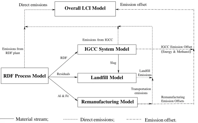
As illustrated in Figure 2-2, the overall LCI model is comprised of multiple

sub-models, including the RDF process model, the IGCC system model, the landfill model,

and the remanufacturing model. An ammonia process model was developed by Xie, 2000.

However, it has not been integrated with the entire system. Therefore, the effect of the

ammonia production on the LCI of the gasification system can not be estimated in this

study.

The essential feature of LCI methodology is an attempt to thoroughly consider all

aspects of a process. In the context of gasification of MSW, the LCI methodology requires

that in addition to an inventory of the direct emissions associated with the RDF plant, the

transportation from the RDF to the remanufacturing plant, the IGCC system, the traditional

landfill, and the ash landfill, an inventory of the avoided emissions is also included. This

accounts for the avoided emissions associated with the recovery of recyclable materials

(ferrous and aluminum), and the production of methanol, electricity, ammonia and sulfur

from syngas. An offset analysis was used to capture the benefit of recyclables recovery,

Overall LCI Model

RDF

Process

Model

IGCC

System

Model

Landfill

Model

Remanufacturing

Model

Residuals Emissions from

RDF plant

RDF

Al & Fe

EmissionsfromIGCC

Landfill Emissions

Direct emissions

Emission offset

IGCCEmissionOffset

(

)

Material stream;

_Direct

_emissions;

_Emission

_offset

Transportation emissions Slag

aluminum is converted to a new product, there are emissions associated with the

manufacturing process. There are also emissions that are avoided because the aluminum

product is not produced from virgin materials. In an offset analysis, the emissions from the

virgin process are subtracted from the emissions from the recycle process and the net value

is added to the overall system LCI. This net value is a negative number if the recovery

process is beneficial. The overall LCI model integrates all the sub models and calculates

the LCI of the direct emissions and the avoided emissions for the entire MSW/coal blends

gasification process.

2.2.1 Overview of the IGCC Based Polygeneration System Model

Gasification is a technology that has been widely used in commercial applications

for over 40 years in the production of fuels and chemicals. Current trends in the chemical

manufacturing and petroleum refinery industries indicate that use of gasification facilities

to produce syngas will continue to increase (Orr, et. al, 2000). Attractive features of the

technology include: 1) the ability to produce a consistent, high quality syngas product

composed primarily of carbon monoxide and hydrogen, which can be used as a fuel to

generate electricity, steam and/or used as a basic chemical building block in the

petrochemical and refining industries; and 2) the ability to accommodate a wide variety of

gaseous, liquid, and solid feedstocks. Gasification regained attention in 1970’s due to the

energy crisis in the US at that time.

An IGCC system is one system that utilizes gasification technology to produce

power. It replaces the traditional coal combustor with a gasifier and gas turbine. Exhaust

heat from the gas turbine is used to produce steam for a conventional steam turbine, thus

the gas turbine and steam turbine operate in a combined cycle. The IGCC configuration

provides high system efficiencies and ultra-low pollution levels compared to conventional

power generation systems (Orr

et. al

, 2000). In addition to electricity, the syngas produced

in a gasification plant can also be used to produce industrial feedstocks including methanol,

IGCC equivalent. (Simbeck, 2001). In Table 2-1, the top 10 commercial gasification

projects are presented.

Table 2-1 Top 10 Commercial Gasification Projects (Simbeck, 2001)

Plants

Location Gasifiers MW syngas Year

Feedstock/Products

Sasol-

Π

S. Africa Lurgi

5,090

1977

Coal/F-T liquids

Sasol-Ø

S. Africa Lurgi

5,090

1982

Coal/F-T liquids

Confidential*

USA

Texaco

2,761

2006

Coal/Electric

Port Authur*

USA

E-Gas

2,029

2005

Coal/Electric

Dakota

USA

Lurgi

1,900

1984

Lignite/SNG

Repsol*

Spain

Texaco

1,654

2005

Residue/Electric

Lake Charles* USA

Texaco

1,407

2005

Coke/Electric

Deer Park*

USA

Texaco

1,400

2006

Coke/Electric

Eagle Energy* USA

Texaco

1,367

2005

Coke/Electric

SARLUX

Italy

Texaco

1,217

2001

Residue/Electric

* Planned

2.2.1.1 Introduction to ASPEN PLUS Software

In this study, the gasification process is simulated as an IGCC system model by

using a chemical software, ASPEN (Advanced Systems for Process Engineering) PLUS.

ASPEN PLUS is a chemical process simulation software that enables users to design and

simulate a process. ASPEN PLUS can estimate material and energy balances, phase and

equilibrium, physical properties of chemical compounds and even the capital cost of

equipment. With users’ inputs, reliable thermodynamic data, realistic operating conditions,

and rigorous equipment models, it can model, control, optimize and manage a steady-state

chemical process (ASPEN Tech 2000). ASPEN PLUS 10.1-0, which runs on Windows 98

platform and incorporates a Graphic User Interface (GUI), was employed to develop and

implement the IGCC model.

2.2.1.2 Overview of the IGCC System Model

The IGCC system model, which calculates mass and energy balances for the entire

IGCC system, was developed by Pickett (2000) and Vaswani (2000). In this study, this

model was calibrated to the MSW/coal blends as described in Appendix C. The model

auxiliary power requirements for each process area and for supporting facilities are also

modeled.

The gasification island consists of the gasification area, the gas cooling/cleaning

and liquor separation area, and the sulfur recovery area. In the gasification island, clean

syngas is produced and then used as the feedstock to produce energy in the power island or

to produce chemicals such as methanol and ammonia. A simplified schematic of the

gasification island is illustrated in Figure 2-3.

The gasification area is based on a British Gas/Lurgi (BGL) slagging gasifier. As

modeled, the fuel in the gasification area is first converted to a form that can be processed

by ASPEN PLUS. Then the hydrocarbons that enter the combustion zone are generated

from the carbon, hydrogen, and oxygen. In this process, some carbon and sulfur are taken

out of the fuel and are added to the slag. In the combustion zone, carbon and oxygen are

partially combusted and the resulting products enter the gasifier for gasification. The crude

syngas generated in the gasifier is then separated from ash and CaO and enter the gas

cooling area.

To simulate the gasification of solid materials such as MSW in ASPEN PLUS, an

ultimate analysis, a proximate analysis, and the sulfur content must be specified. For RDF,

these values were calculated in the RDF process model which is described in section 2.2.3.

For coal, these values were obtained from the literature (Pechtl

et al.

, 1992).

Crude syngas is then cooled before it enters the gas cleaning area. The gas cooling

section is highly integrated with the rest of the IGCC system. Water used to cool the syngas

is from the fuel gas saturation area and steam cycle.

The gas cleaning section utilizes the Rectisol® cleaning process to remove sulfur

and other contaminants from the syngas. The Rectisol® cleaning unit separates the cooled

syngas into a clean gas, an acid gas, a naphtha rich gas, a condensate and a CO

rich gas.

The gas liquor separation area separates the combustible hydrocarbons from water

Figure 2-3 Simplified Schematic of Gasification Island of IGCC System

Gasifier

Gas

Cooling/Cleanin

g

Acid Gas

Separator

Air Separation

Plant

RDF

Coal

Electricity

Emissions

(

H2S

)

N

O

Claus Plant

Tail Gas

Treatment

Liquor

Separation

Slag

Steam

Combustible _Hydrocarbons

Sulfur

Material Stream; Electricity Stream

in the process condensate are separated and recycled to the gasifier. While the other stream

containing the gases dissolved in the liquor proceeds to the Beavon-Stretford tail-gas

treatment process. The remaining liquid is split for use in the quench units in the

gasification area and gas cooling section.

The sulfur recovery section consists of a Claus plant and a Beavon-Stretford tail gas

treatment plant. In the Claus plant, sulfur is recovered from H

S while a tail gas of SO

is

also generated. The tail gas is further treated in the Beavon-Stretford tail gas treatment

plant to recover sulfur from SO

.

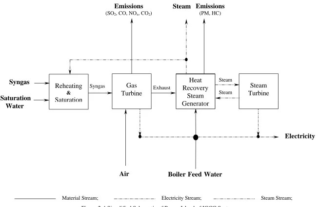
After the removal of impurities and sulfur containing compounds, the syngas enters

the saturation area. In the power island, the clean syngas is saturated with water to reduce

NO

emissions and increase power output from the gas turbine. After saturation in the fuel

gas saturation area, the outlet stream is advanced to gas turbine. The heat of the exit gas

from the gas turbines is recovered as steam. A simplified schematic of power island is

illustrated in Figure 2-4.

The gas turbines modeled for the IGCC system represent a heavy-duty “F” class

system, similar to a General Electric MS7001F. The default assumed IGCC plant size

includes two gas turbines in parallel (Pickett, 2000). The gas turbine consists of three

sections; compression, combustion and expansion. The compression section pressurizes

and heats air. Cooling air is extracted from the compression section to cool the expander

blades and rotors with air, thereby prolonging the life of the expanders. The fuel, along

with compressed air, is introduced to the combustion section. After combustion, the hot,

compressed exhaust gas expands to generate electrical energy.

The steam cycle consists of two sections: the heat recovery steam generator

(HRSG) and the steam turbine. The HRSG cools the exit gas from the gas turbine and

recovers the sensible heat in steam production. Liquid water enters the steam cycle process

area to generate high-pressure, intermediate-pressure, and low-pressure steam. There are

four HEATER blocks in HRSG to cool the exhaust gas of the gas turbine and to provide

Figure 2-4 Simplified Schematic of Power Island of IGCC System

Material Stream; Electricity Stream; Steam Stream;

Boiler

Feed

Water

Electricity

Steam

Reheating

Saturation

Syngas

Emissions

Syngas _Exhaust

Steam

Turbine

Steam

Saturation

Water

Gas

Turbine

Air

Emissions

Heat

Recovery

There are three stages in the steam turbine. The super-heated, high-pressure steam

enters the first stage of the steam turbine. Its pressure is reduced in the first stage and then it

mixes with the intermediate-pressure steam. The mixture advances to the second stage of

the steam turbine. The outlet stream is mixed with low-pressure steam and the mixture

enters the final stage of the steam turbine.

2.2.1.3 Overview of Liquid Phase Methanol Process and Conventional Methanol

Production Model

A Liquid Phase Methanol Process (LPMEOH

) model was developed and

integrated with the IGCC model (Vaswami 2000, Pickett, 2000). The LPMEOH

model

simulates the production of methanol from syngas produced by the MSW/coal blends

gasification. In addition to syngas, the steam produced during gasification is used in

methanol production. The process model consists of twenty-six unit operation blocks, four

FORTRAN blocks and four design-specs (Vaswani 2000).

To calculate the offset LCI of the methanol produced by the gasification system, a

model for calculation of the LCI of the methanol produced using conventional technology

was required. This model was also developed by Vaswani (2000). It was modeled based on

conventional feedstock (natural gas). Coefficients were calculated from mass and energy

balance as well as consideration of overall energy requirements. The offset LCI

coefficients for the conventional methanol process are presented in Table B-1.

2.2.2 Overview of Waste to Energy Model

The objective of the waste-to-energy process model is to calculate the cost and LCI

for a MSW WTE facility. A detailed description of the WTE-LCI model has been

presented previously (Harrison et al. 2000). In this study, the LCI portion of the

waste-to-energy model was used to calculate the LCI associated with MSW combustion.

LCI parameters are calculated on the basis of both user input and default design

information. Model results are based on both the quantity and composition of the waste

combustion. For SO

, NO

, CO and particulate matter, emissions were calculated from

information on regulatory requirements for MSW combustion. In addition, the direct

emissions associated with the transportation from the WTE facility to the remanufacturing

plant were calculated. The WTE-LCI model also computes the avoided emissions due to

energy recovered by MSW combustion. Avoided emissions were calculated by assuming

that any energy recovered offsets the use of natural gas and coal (Harrison et al., 2000). In

this study, the fuel mix of the Southeastern Electric Reliability Council (SERC) was used.

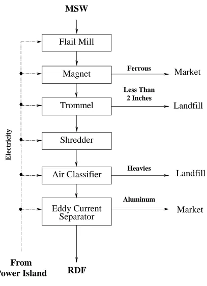
2.2.3 Overview of RDF Process Model

The objective of the RDF process model is to calculate the energy consumption and

LCI parameters for converting MSW into a fuel that is used to produce syngas by

gasification. The conceptual design of the RDF model is illustrated in Figure 2-5. A

detailed description of the RDF process model with all equations is presented in Appendix

A and an overview of the model is presented below. All input default values are also

presented in Appendix A.

In the modeled RDF facility, refuse that is received either loose or in bags is loaded

onto a conveyor and fed to a flail mill. The flail mill opens any unopened bags and reduces

the size of some of the refuse. From the flail mill, the refused passes under a magnet that

recovers ferrous metal. The remaining refuse then continues to a trommel for removal of

material less than 2 inches in diameter. The trommel removes materials like broken glass,

dirt, and some food waste, all of which have a low energy value. From the trommel, refuse

is shredded and then routed to an air classifier that separates the “lights”, considered to

have the high BTU content, from the “heavies”, which have a relatively low BTU content.

The “lights” then flow to an eddy current separator for aluminum removal. The material

Electricity

MSW

Magnet

Trommel

Shredder

Air Classifier

Ferrous

Less Than

2 Inches

Heavies

Landfill

Flail Mill

From

Power Island

Landfill

Market

Eddy Current

Separator

Aluminum

Market

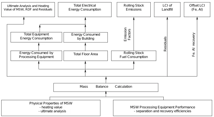
The calculation sequence for the RDF process model is illustrated in Figure 2-6.

The quantity and composition of materials flowing through the RDF plant, including the

RDF stream, the residual stream, and the recovered ferrous and aluminum, are calculated

through mass balance equations based on assumed separation efficiencies at each step.

Energy is consumed in the production of RDF both by processing equipment such as the

shredder and by rolling stock. Thus, both diesel fuel and electrical energy are consumed.

For each type of energy, both combustion energy and precombusiton energy is considered.

Combustion energy is the energy consumed directly (diesel or electricity), while

precombustion energy is the energy that is required to produce the combustion energy. The

ultimate analysis of RDF is a required input to the IGCC model and is calculated based on

the ultimate analysis of each MSW component and a mass balance through the RDF plant.

The LCI associated with the RDF process contains three parts: diesel combustion in rolling

stock; pre-combustion emissions associated with diesel production; and emissions

associated with electrical consumption. The benefits associated with the recovered

aluminum and ferrous are calculated in the remanufacturing process model.

The LCI coefficients for the RDF process model are presented in Table B-2.

2.2.4 Overview of the Landfill Model

The objective of the landfill process model is to calculate the cost and LCI for a

landfill. The landfill process model is a sub-model of the ISWM model. Only the LCI

results were used for this study.

In the RDF production process, the low heating value materials that are referred to

as residuals are managed in a traditional landfill. The landfill process model was used to

evaluate two scenarios, a landfill with or without energy recovery. For the landfill with

energy recovery, energy was recovered by the conversion of methane to electrical energy

in a turbine.

Avoided emissions associated with electrical energy production were handled

as for the WTE-LCI model. In this study, the fuel mix of the SERC was used, which is the

Mass Balance Calculation Energy Consumed by

Processing Equipment

Rolling Stock Fuel Consumption Total Floor Area

Total Equipment Energy Consumption

Energy Consumed by Building Total Electrical Energy Consumption

Offset LCI (Fe, Al)

Physical Properties of MSW - heating value - ultimate analysis

Ultimate Analysis and Heating Value of MSW, RDF and Residuals

Rolling Stock Emissions

LCI of Landfill

Emission Factors

Residuals

Fe. Al recovery

MSW Processing Equipment Performance - separation and recovery efficiencies

it is managed in an ash landfill. There are environmental emissions associated with the

landfill treatment of the residuals and slag.

The landfill process model simulates landfill operation based on default design

information and user inputs. In this study, the LCI coefficients of the traditional and ash

landfill are used to compute the environmental burdens for the disposal of the MSW

residuals and the slag from the IGCC system. A detailed description of the landfill process

model is presented in Sich (1999). The LCI coefficients for the traditional landfill

with/without energy and the coefficients for the ash landfill are presented in Table B-3, B-4

and B-5, respectively.

2.2.5 Overview of Transportation Model

The objective of the transportation model is to calculate the LCI coefficients for

transporting the recovered ferrous and aluminum from the recovery units such as the RDF

plant to the remanufacturing plants. The transportation model is a sub-model of the ISWM

model. In this study, it was used to calculate the recovered ferrous and aluminum

transportation associated emissions from both the RDF plant and the WTE plant to the

remanufacturing plant. The assumed distances to the remanufacturing plant and the

transportation associated LCI coefficients for the RDF plant and the WTE plant are

presented in Table B-6, and Table B-7, respectively.

2.2.6 Overview of Remanufacturing Model

The objective of the remanufacturing model is to calculate emission offsets

associated with the recovery of recycled aluminum and ferrous. The remanufacturing

model is a sub-model of the ISWM model. One ton ferrous or aluminum can be produced

either by virgin material or by recycled material. If virgin material is used to produce one

ton ferrous or aluminum, there are energy consumption and environmental emissions

associated with the processes of mining, combustion, and transportation, which will be

avoided if recycled materials are used. Therefore, there exist offset LCIs when ferrous and

aluminum are recovered for remanufacturing. The offset is calculated as the difference in

emissions between the manufacturing processes based on virgin and recycled materials.

3.0 CASE STUDIES ON THE APPLICATION OF GASIFICATION

TECHNOLOGY TO MSW

This chapter presents the results of case studies on the application of gasification

technology to MSW. Three scenarios were defined to analyze the gasification system. In

addition to the results for these scenarios, sensitivity analyses were conducted on the LCI

model based on the base case.

3.1 Scenario Definition

Three scenarios were designed to evaluate the LCI of MSW gasification. The IGCC

plant size was varied in each scenario by varying methanol production. The size of the

methanol production plant was set at 10,000, 20,000 and 40,000 lb/hr in scenarios A, B and

C, respectively. In each scenario, the size of the two gas turbines modeled in the IGCC

system model is constant.

For each scenario, a series of model runs was made to determine (1) material usage,

material production, energy production, and the emissions associated with the RDF/coal

blends, (2) the material usage, the material production, the energy production and the

emissions that could be attributed to RDF production and (3) the environmental burdens

associated with the application of gasification technology to MSW. For each of the three

scenarios, two cases are considered. In case 1, the MSW residual is disposed in a traditional

landfill with no energy recovery. In case 2, the MSW residual is disposed in a traditional

landfill with electrical energy recovery. The landfill gas (LFG) is treated differently in

these two cases, as listed in Table 3-1.

As developed, the IGCC model allows for calculation of the LCI for the MSW/coal

blend. However, it was necessary to separate out the fraction of the LCI that was

attributable to MSW. This is because in Chapter 4, the LCI of MSW gasification is

compared to that of WTE that processes MSW without coal. The allocation technique is

Table 3-1 LFG Treatment in the First, Second, Third Treatment Periods in Case 1 & 2

Landfill Gas Treatment Methods

Case 1 (%)

Case 2 (%)

Year 1 - 5

Flare 100 0

Year 6 - 40

Turbine 0 100

Flare 100 0

Year 41 - 80

Turbine 0 100

3.2 Input Assumptions and Results of the Base Case

The calculation sequence for the LCI model is as follows.

1. Use the RDF process model to compute the proximate analysis, ultimate

analysis and the heating value of the RDF based on the user specified MSW

composition and physical properties.

2. Use the IGCC system model to compute the material usage, material

production, and energy production with a specified RDF/coal blend and

methanol plant size.

3. Use the RDF process model, the IGCC model, the landfill model, the electricity

model, the remanufacturing model and the conventional methanol production

model to compute the total LCI of the MSW/coal blends system.

In the base case, the RDF/coal blend is specified on the weight average with 25%

Pittsburgh #8 coal and 75% RDF. The methanol plant size is set to produce 10,000 lb

methanol /hr.

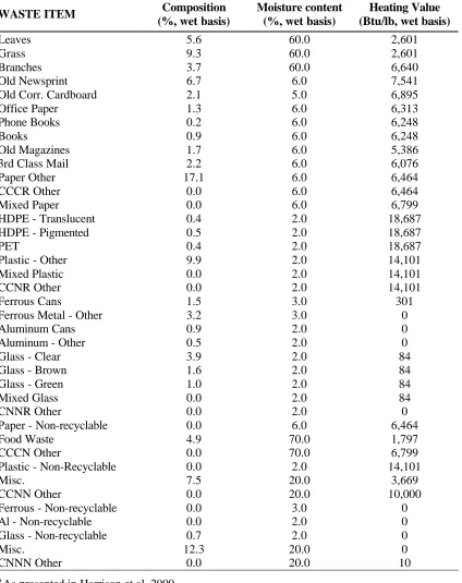
3.2.1 MSW Waste Composition

The MSW waste stream used in the base case is characterized by 39 waste

Table 3-2 Waste Composition and Heating Value of Each MSW Component

WASTE ITEM Composition

(%, wet basis)

Moisture content (%, wet basis)

Heating Value (Btu/lb, wet basis)

Leaves 5.6 60.0 2,601

Grass 9.3 60.0 2,601

Branches 3.7 60.0 6,640

Old Newsprint 6.7 6.0 7,541

Old Corr. Cardboard 2.1 5.0 6,895

Office Paper 1.3 6.0 6,313

Phone Books 0.2 6.0 6,248

Books 0.9 6.0 6,248

Old Magazines 1.7 6.0 5,386

3rd Class Mail 2.2 6.0 6,076

Paper Other 17.1 6.0 6,464

CCCR Other 0.0 6.0 6,464

Mixed Paper 0.0 6.0 6,799

HDPE - Translucent 0.4 2.0 18,687

HDPE - Pigmented 0.5 2.0 18,687

PET 0.4 2.0 18,687

Plastic - Other 9.9 2.0 14,101

Mixed Plastic 0.0 2.0 14,101

CCNR Other 0.0 2.0 14,101

Ferrous Cans 1.5 3.0 301

Ferrous Metal - Other 3.2 3.0 0

Aluminum Cans 0.9 2.0 0

Aluminum - Other 0.5 2.0 0

Glass - Clear 3.9 2.0 84

Glass - Brown 1.6 2.0 84

Glass - Green 1.0 2.0 84

Mixed Glass 0.0 2.0 84

CNNR Other 0.0 2.0 0

Paper - Non-recyclable 0.0 6.0 6,464

Food Waste 4.9 70.0 1,797

CCCN Other 0.0 70.0 6,799

Plastic - Non-Recyclable 0.0 2.0 14,101

Misc. 7.5 20.0 3,669

CCNN Other 0.0 20.0 10,000

Ferrous - Non-recyclable 0.0 3.0 0

Al - Non-recyclable 0.0 2.0 0

Glass - Non-recyclable 0.7 2.0 0

Misc. 12.3 20.0 0

CNNN Other 0.0 20.0 10

a

3.2.2 Input Assumptions for the Base Case

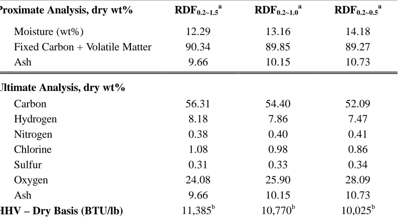
Table 3-3 provides the proximate analysis, ultimate analysis, and the higher heating

value of the RDF/coal blend that will be fed into the IGCC system. They are the weighted

average of 25% Pittsburgh #8 coal and 75% RDF. The data for RDF was computed in the

RDF process model based on the MSW specified in Table 3-2. The heating value for the

RDF/coal blends used in this study was calculated by Dulong correlation equation instead

of by the RDF process model to account for the uncertainty and variability in the RDF

process model inputs and parameters.

Table 3-3. Proximate and Ultimate Analysis of Pittsburgh No. 8 Coal, RDF, and RDF/coal

blend

Proximate Analysis, dry wt% Pittsburgh No. 8

RDF RDF/coal blend

Moisture (wt %) 6.00 14.42 13.32

FC & VMc 87.77 86.54 86.87

Ash 12.23 13.46 13.13 Ultimate Analysis, dry wt%

Carbon 73.21 46.96 53.99 Hydrogen 4.94 6.39 6.00 Nitrogen 1.38 0.58 0.79 Chlorine 0.00 1.19 0.87 Sulfur 3.39 0.41 1.21 Oxygen 4.85 31.01 24.00 Ash 12.23 13.46 13.13

HHV – Dry Basis (BTU/lb) 13,138 9,658

9,738

a

Pechtl et al., 1992

b

The RDF/coal blend is comprised of 25% of Pittsburgh #8 coal and 75% of RDF

FC – Fixed Carbon and VM – Volatile Matter

HHV calculated from the ultimate analysis using the Dulong correlation

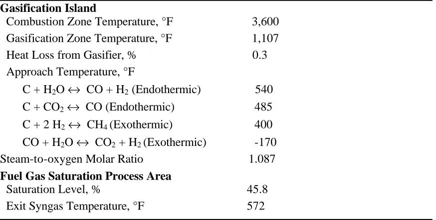
The input assumptions for the IGCC system firing the MSW/coal blends are

presented in Table 3-4. The input assumptions were developed based on a review of design

and performance parameters obtained from the literatures (Pickett, 2000). A detailed

Table 3-4. Input Assumptions for the IGCC System Firing the RDF/coal blend

Gasification Island

Combustion Zone Temperature, °F 3,600

Gasification Zone Temperature, °F 1,107

Heat Loss from Gasifier, % 0.3

Approach Temperature, °F

C + H

O

↔

CO + H

(Endothermic) 540

C + CO

↔

CO (Endothermic) 485

C + 2 H

↔

CH

(Exothermic) 400

CO + H

O

↔

CO

+ H

(Exothermic) -170

Steam-to-oxygen Molar Ratio 1.087

Fuel Gas Saturation Process Area

Saturation Level, % 45.8

Exit Syngas Temperature, °F 572

a – The input assumptions for the IGCC system firing RDF/coal blends were calibrated in Appendix C.

3.2.3 The LCI Model Results for the Base Case

3.2.3.1 The Results of the IGCC Based Polygeneration System Model

After specifying the input RDF/coal blend and the input assumptions for the IGCC

system, the IGCC model is used to compute data for the LCI calculation of the MSW/coal

gasification system, including total material usage, total material production, total power

production, and total emissions from IGCC system when firing RDF/coal blends and

producing 10,000 lb/hr methanol. The contribution of the RDF to the total material flows,

energy flows, and emissions is also computed. The contribution of the RDF was

calculated based on the contribution of the RDF to the total energy input, except two cases:

1) The contribution of the RDF to the fuel, which is calculated based on the weight

percentage of RDF and coal; 2) The contribution of the RDF to the ash and sulfur, which is

calculated based on the ratio of the ash and sulfur content in the RDF to the ash and sulfur

content in the RDF/coal blends. The calculation is given by Equation 3-1. The basis for this

calculation is that material production, energy production, and emissions are related to the

Where:

MRDF -- Contribution factor for RDF for material usage, material production, energy production, and emissions (Lb/hr or kWh/hr)

MTotal -- Total material usage, material production, energy production, and emissions (Lb/hr or kWh/hr)

E_inputRDF -- Contribution of RDF to the total energy input. E_inputRDF = 75% x Fuel_Input x HHVwet of RDF E_inputTotal -- Total energy input

E_inputTotal = Fuel_Input x (75% x HHV wet

of RDF + 25% x HHVwet of coal) HHVwet – Higher heating value on wet basis

For the LCI, CO

is categorized into fossil CO

and biomass CO

. However, the

IGCC system model only calculates the sum of these two types of CO

. Therefore, the CO

emission must be categorized. This was done based on Table 3-5.

Table 3-5 Categorization of Waste Items with Respect to CO

Emission Source

Waste Item Biomass CO2 Fossil CO2

Leaves X

Grass X

Branches X

Old Newsprint X

Old Corr. Cardboard X

Office Paper X

Phone Books X

Books X

Old Magazines X

3rd Class Mail X

Paper Other X

CCCR Other X

Mixed Paper X

HDPE - Translucent X

HDPE - Pigmented X

PET X

Plastic - Other X

Mixed Plastic X

CCNR Other X

Ferrous Cans X

Ferrous Metal - Other X

Aluminum Cans X

1)

-3

(Eqn

input

_

E

input

_

E

M

M

(Continued)

Waste Item Biomass CO2 Fossil CO2

Aluminum - Other X

Glass - Clear X

Glass - Brown X

Glass - Green X

Mixed Glass X

CNNR Other X

Paper - Non-recyclable X

Food Waste X

CCCN Other X

Plastic - Non-Recyclable X

Misc. X

CCNN Other X

Ferrous - Non-recyclable X

Al - Non-recyclable X

Glass - Non-recyclable X

Misc. X

CNNN Other X

Selected results of the IGCC system model that will be used for calculation of the

LCI for the gasification system for the base case are summarized in Table 3-6, including

fuel, methanol, sulfur, slag, and power flow rate and emissions from the IGCC system.

Table 3-6 Selected Results of the IGCC System Model for the Base Case

RDF/coal blend Contribution of RDF Material

Methanol (lb/hr) 10,000 6,354

Fuel (lb/hr) 481,969 361,476

Sulfur (lb/hr) 5,164 2,292

Slag (lb/hr) 69,862 61,442

Power

Power to Grid (MW) 452.6 287.6

Emissions

SO2 (lb/hr) 9.40E-01 7.17E-03

CO2 (Biomass) (lb/hr) 4.21E+05 3.21E+03

CO2 (Fossil) (lb/hr) 3.17E+05 2.42E+03

NOx (lb/hr) 388.5 2.96E+00

3.2.3.2 Material and Energy Flows of the MSW/Coal Blends Gasification System

Based on the RDF demand calculated in section 3.2.3.1, the MSW demand to the

gasification system for the base case, and the MSW residual produced, the ferrous &

aluminum recovered and the power consumed associated with such amount of MSW are

calculated by using the RDF process model. Hence, the material and energy flows for

calculation of the LCI of the gasification system for the base case are calculated and

summarized in Table 3-7.

Table 3-7 Material and Energy Flows Attributed to RDF of the MSW/Coal Blends

Gasification System

MSW Input (Ton/day) 7,776

RDF Produced (Ton/day) 4,338

MSW Residual (Ton/day) 3,012

Fe Recovered (Ton/day) 329

Al Recovered (Ton/day) 98

Slag from IGCC (Ton/day) 737

Sulfur Produced (Ton/day) 28

Methanol Produced (Ton/day) 76

Power Consumed in RDF Plant (MWh/day) 391

Net Power from IGCC (MWh/day) 6902

These material and energy flows provide the basis for calculation of the LCI of the

MSW/coal gasification system. The MSW feed rate will determine emissions from the

RDF plant; the MSW residual is assumed to be buried in a traditional landfill and results in

emissions from disposal; the slag from IGCC assumed to be buried in an ash landfill and

results in emissions from disposal; the power consumption in RDF plants is subtracted

from the power produced in the IGCC system, which results in the net power production of

the overall system. There are avoided emissions associated with the methanol production,

sulfur production, ferrous and aluminum recovered, and net power production of the

gasification system. The avoided emissions associated with the sulfur production are not

overestimate of emissions since the emissions avoided from conventional sulfur

production are not subtracted.

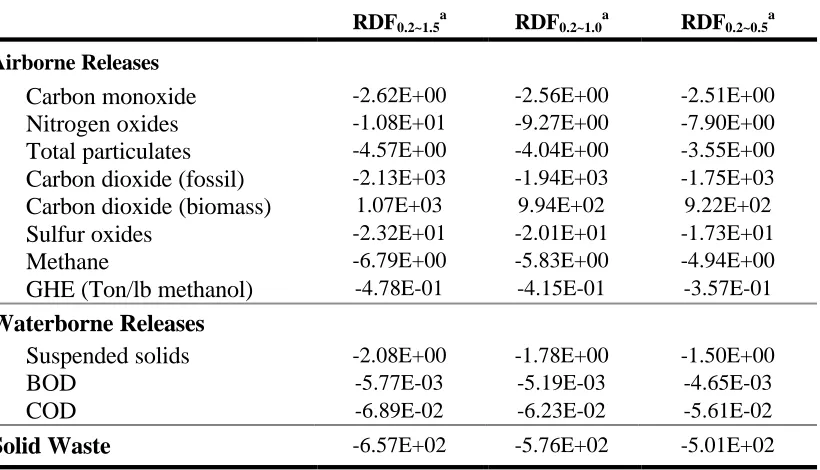
3.2.3.3 The LCI Results of the MSW/Coal Blends Gasification System (Base Case)

The results of the overall LCI for an MSW gasification system for the base case are

presented in Tables 3-8 and 3-9 for a landfill with and without energy recovery,

respectively.

In both cases, for all the pollutants including atmospheric, waterborne and solid

waste emissions, the total emissions are negative, with the exception of biomass CO

and

BOD. The reason is that the emission offsets of the electricity, the aluminum and the

ferrous make the largest contribution to the total emissions of the gasification system LCI.

While for Biomass CO

, the largest contributor to its emission is the direction emissions

from the IGCC based polygeneration system. For BOD, the largest contributor to its

emission is the direction emissions associated with the MSW disposal in the landfill. The

reason is due to the lechate release from the landfill. A lechate collection system efficiency

of 99% was assumed for the landfill process model so that 1% of lechate generated is also

released to the environment directly. Both treated and untreated lechate releases are

included in the landfill emissions presented in Tables 3-8 and 3-9.

The emissions in Case 2 are less than those in Case 1 because in case 2 the LFG

from traditional landfill is converted to energy and there are avoided emissions associated

with the recovered energy. However, the difference between landfill with and without

energy recovery is negligible to the total emissions. This is partly due to largest contributor

to the total emissions of most pollutants is the offset emissions associated with the

electricity, aluminum and ferrous, instead of the direction emissions from the landfill.

Another reason is due to the fact that paper is the largest biodegradable component of

MSW and paper is in the RDF used for gasification, and not in the residual stream.

Because the emission offsets of sulfur are not considered, the total emissions of the

One assumption was made for the offset emissions associated with the methanol

production that the biomass CO

emission is zero because in conventional methanol plants,

Table 3-8 LCI Results of the MSW/Coal Blends Gasification System (Base Case / Landfill with no Energy Recovery)

(Lbs/day)

Coal Precomb.

IGCC Plant

RDF Plant

Traditional Landfill

Ash Landfill

Electricity Offset

Methanol

OffsetC Transportd

(Al + Fe)

Offset Total

Airborne Releases

Carbon monoxide 1.30E+02 3.23E+03 2.83E+02 1.23E+02 1.84E+01 -3.87E+03 -1.15E+03 1.77E+02 -1.80E+04 -1.91E+04 Nitrogen oxides 1.66E+02 5.92E+03 4.40E+02 1.95E+01 5.43E+01 -5.12E+04 -5.43E+02 1.79E+02 -6.30E+03 -5.13E+04 Total particulates 1.85E+03 3.60E+02 4.87E+01 1.37E+01 4.99E+00 -1.75E+04 -8.42E+01 2.58E+01 -8.63E+03 -2.39E+04 Carbon dioxide (fossil fuel) 2.94E+04 4.81E+06 7.09E+03 1.06E+03 3.88E+03 -1.36E+07 -2.39E+05 2.09E+04 -2.75E+06 -1.17E+07 Carbon dioxide (biomass fuel) 2.17E+02 6.46E+06 7.15E+04 1.21E+05 9.15E-01 -1.92E+03 0.00E+00 5.00E+00 0.00E+00 6.65E+06

Sulfur oxides 1.66E+02 1.43E+01 1.03E+02 5.12E+00 9.24E+00 -9.05E+04 -5.60E+03 5.08E+01 -1.78E+04 -1.14E+05 Hydrocarbons 6.15E+01 3.12E+02 2.02E+02 3.06E+00 1.39E+01 -2.63E+03 N/A 7.21E+01 -3.21E+03 N/A

Methane 3.39E+03 N/A 1.09E+01 1.06E+03 6.88E-01 -3.00E+04 -1.35E+03 3.32E+00 -3.76E+03 -3.06E+04 Lead 1.95E-03 N/A 3.78E-04 1.50E-05 2.10E-05 -5.84E-01 N/A 1.15E-04 4.04E-01 N/A Ammonia 6.29E-02 N/A 1.08E-01 2.41E-03 6.00E-03 -1.14E+01 N/A 3.28E-02 -6.45E+00 N/A Hydrochloric acid 7.95E-01 N/A 6.75E-02 1.59E+00 4.64E-03 -1.10E+03 N/A 2.05E-02 -3.87E+02 N/A

GHEe (Tons/day) 1.37E+01 N/A 9.98E-01 3.18E+00 5.31E-01 -1.94E+03 -3.65E+01 2.86E+00 -3.86E+02 -2.34E+03

Waterborne Releases

Dissolved Solids 5.93E+01 N/A 9.39E+01 1.41E+00 5.22E+00 -1.15E+04 N/A 2.85E+01 -9.47E+03 N/A Suspended solids 1.02E+03 N/A 2.13E+00 1.98E-01 2.09E-01 -9.56E+03 -5.14E+01 6.48E-01 -1.03E+03 -9.62E+03 Bio-chemical Oxygen Demand 8.68E-02 N/A 3.51E-01 3.41E+01 3.98E-02 -1.14E+01 -7.47E+00 1.07E-01 -1.41E+01 1.69E+00

(Continued)

Coal Precomb.

IGCC Plants

RDF Plant

Traditional Landfill

Ash Landfill

Electricity Offset

Methanol

OffsetC Transportd

(Al + Fe)

Offset Total

Cadmium 2.60E-03 N/A 3.51E-03 5.86E-05 1.95E-04 -5.22E-01 N/A 1.07E-03 -4.02E-01 N/A Arsenic 0.00E+00 N/A 0.00E+00 2.10E-05 0.00E+00 0.00E+00 N/A 0.00E+00 0.00E+00 N/A Mercury 2.02E-07 N/A 2.64E-07 2.97E-07 1.47E-08 -4.10E-05 N/A 8.03E-08 -3.60E-04 N/A Phosphate 8.68E-02 N/A 9.44E-03 7.95E-03 5.25E-04 -6.76E+01 N/A 2.87E-03 -3.79E+00 N/A Selenium 0.00E+00 N/A 0.00E+00 6.79E-06 0.00E+00 0.00E+00 N/A 0.00E+00 0.00E+00 N/A Chromium 2.60E-03 N/A 3.51E-03 1.13E-04 1.95E-04 -5.22E-01 N/A 1.07E-03 -4.02E-01 N/A Lead 4.12E-06 N/A 4.05E-05 9.76E-06 2.25E-06 -3.86E-05 N/A 1.23E-05 -2.08E-03 N/A Zinc 9.40E-04 N/A 1.75E-03 2.58E-05 9.75E-05 -1.79E-01 N/A 5.33E-04 -1.45E-01 N/A

Solid Waste 2.49E+05 N/A 3.59E+02 1.83E+02 2.79E+01 -2.60E+06 -2.91E+04 1.09E+02 -9.53E+05 -3.33E+06 a

The term “N/A” means that data for that item are not available.

b

Based on material flows given in Table 3-7.

c

This is offset from net energy production from IGCC based polygeneration system after subtracting the RDF plant demand.

d

LCI associated with the transportation from RDF plants to remanufacturing plants

Table 3-9 LCI Results of the MSW/Coal Blends Gasification System (Base Case / Landfill with Energy Recovery)

(Lbs/day)

Coal Precomb.

IGCC Plant

RDF Plant

Traditional Landfill

Ash Landfill

Electricity Offset

Methanol

OffsetC Transportd

(Al + Fe)

Offset Total

Airborne Releases

Carbon monoxide 1.30E+02 3.23E+03 2.83E+02 3.90E+01 1.84E+01 -3.87E+03 -1.15E+03 1.77E+02 -1.80E+04 -1.91E+04 Nitrogen oxides 1.66E+02 5.92E+03 4.40E+02 2.32E+00 5.43E+01 -5.12E+04 -5.43E+02 1.79E+02 -6.30E+03 -5.13E+04 Total particulates 1.85E+03 3.60E+02 4.87E+01 -1.11E+01 4.99E+00 -1.75E+04 -8.42E+01 2.58E+01 -8.63E+03 -2.39E+04 Carbon dioxide (fossil fuel) 2.94E+04 4.81E+06 7.09E+03 -5.42E+03 3.88E+03 -1.36E+07 -2.39E+05 2.09E+04 -2.75E+06 -1.18E+07 Carbon dioxide (biomass fuel) 2.17E+02 6.46E+06 7.15E+04 3.37E+05 9.15E-01 -1.92E+03 0.00E+00 5.00E+00 0.00E+00 6.87E+06 Sulfur oxides 1.66E+02 1.43E+01 1.03E+02 -3.79E+01 9.24E+00 -9.05E+04 -5.60E+03 5.08E+01 -1.78E+04 -1.14E+05 Hydrocarbons 6.15E+01 3.12E+02 2.02E+02 1.81E+00 1.39E+01 -2.63E+03 N/A 7.21E+01 -3.21E+03 N/A

Methane 3.39E+03 N/A 1.09E+01 1.05E+03 6.88E-01 -3.00E+04 -1.35E+03 3.32E+00 -3.76E+03 -3.06E+04 Lead 1.95E-03 N/A 3.78E-04 -2.63E-04 2.10E-05 -5.84E-01 N/A 1.15E-04 4.04E-01 N/A Ammonia 6.29E-02 N/A 1.08E-01 -3.03E-03 6.00E-03 -1.14E+01 N/A 3.28E-02 -6.45E+00 N/A Hydrochloric acid 7.95E-01 N/A 6.75E-02 1.10E+00 4.64E-03 -1.10E+03 N/A 2.05E-02 -3.87E+02 N/A

GHEe (Tons/day) 1.37E+01 N/A 9.98E-01 2.26E+00 5.31E-01 -1.94E+03 -3.65E+01 2.86E+00 -3.86E+02 -2.35E+03

Waterborne Releases

Dissolved Solids 5.93E+01 N/A 9.39E+01 -4.08E+00 5.22E+00 -1.15E+04 N/A 2.85E+01 -9.47E+03 N/A Suspended solids 1.02E+03 N/A 2.13E+00 -4.35E+00 2.09E-01 -9.56E+03 -5.14E+01 6.48E-01 -1.03E+03 -9.63E+03 Bio-chemical Oxygen Demand 8.68E-02 N/A 3.51E-01 3.41E+01 3.98E-02 -1.14E+01 -7.47E+00 1.07E-01 -1.41E+01 1.69E+00 Chemical Oxygen Demand 9.40E-01 N/A 2.35E+00 9.47E+01 2.75E+01 -1.62E+02 -5.31E+01 7.13E-01 -2.13E+02 -3.02E+02