Imaging properties of a rotation-free, arrayed-source micro-computed tomography system

(1)

ABSTRACT

QUAN, ENZHUO. Imaging Properties of a Rotation-Free, Arrayed-Source Micro-Computed Tomography System. (Under the direction of Professor David S. Lalush.)

We study the three-dimensional reconstruction and imaging properties of a proposed rotation-free micro-computed tomography (CT) system. The system uses linear arrays of the carbon-nanotube-based x-ray sources which have ultra-short switch time and are individually addressable. With such sources, the micro-CT system is able to achieve ultra-high temporal resolution, reduce dose, and facilitate gated imaging.

(2)

To accelerate the reconstruction of the proposed micro-CT system, we presented a faster iterative reconstruction algorithm based on the OSC algorithm. Measurements show that the modified version produces fewer streaking artifacts, similar resolution-noise tradeoff in the reconstructed images, and it saves up to 30% CPU time, so we conclude that the MOSC algorithm is an efficient alternative to OSC.

(3)

(4)

Imaging Properties of a Rotation-Free, Arrayed-Source Micro-Computed

Tomography System

by

Enzhuo Quan

A dissertation submitted to the Graduate Faculty of North Carolina State University

in partial fulfillment of the requirements for the Degree of

Doctor of Philosophy

Biomedical Engineering

Raleigh, North Carolina 2009

APPROVED BY:

_________________________ _________________________

Dr.Mohamed Bourham Dr. Caterina Gallippi

__________________________ _________________________

Dr. Jianping Lu Dr. Wesley Snyder

_________________________ Dr. David Lalush

(5)

DEDICATION

(6)

BIOGRAPHY

(7)

ACKNOWLEDGEMENTS

I would like to express my deepest appreciation to my advisor, Dr. David Lalush for his support and guidance throughout my PhD study. Without his patience, encouragement and advisory, the dissertation would be impossible. His insightful suggestions and inspiration not only helped me in my current research, but will also enlighten my future career path.

I would also like to offer my special thanks to my committee members, Drs. Mohamed Bourham, Caterina Gallippi, Jianping Lu, and Wesley Snyder, for their willingness to join my committee and their time to provide beneficial suggestions and comments.

I also appreciate my colleagues, Dr. Otto Zhou, Dr. Jian Zhang, Dr. Guohua Cao, and Ramya Rajaram from the Department of Physics of UNC-Chapel Hill, Dr. Jianping Lu, Dr. Peng Wang, Dr. Huaizhi Geng, Shabana Sultana from Xintek, Gereon Vogtmeier from Philips Research Europe, and Brian Gonzales from NC State University, for their helpful discussions with me during my PhD study.

The computations were performed in the High Performance Computation (HPC) Center of North Carolina State University. The support and assistance from Dr. Gary Howell in HPC center are highly appreciated.

(8)

(9)

LIST OF TABLES

Table 5.1. Geometric parameters for the test geometries ... .99

Table 6.1. Average axial FWHM of the five PSFs obtained with the no-translation and the bi-translation scanning modes under infinitesimal and 100 µm focal spot situations... 144

Table 6.2. Average transaxial FWHM of the five PSFs obtained with the no-translation and the bi-translation scanning modes under infinitesimal and 100 µm focal spot situations. ... 145

(13)

LIST OF FIGURES

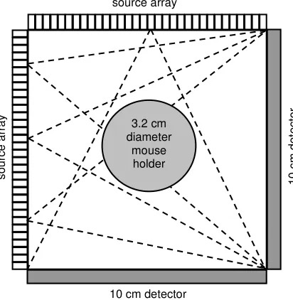
Figure 1.1: Geometry of a proposed rotation-free micro-CT system design, in which two source arrays form two contiguous sides of a square, and two detectors form the other two sides………1

Figure 2.1. X-ray radiation patterns: (a) parallel-beam, (b) fan-beam, and (c) cone-beam.………..8

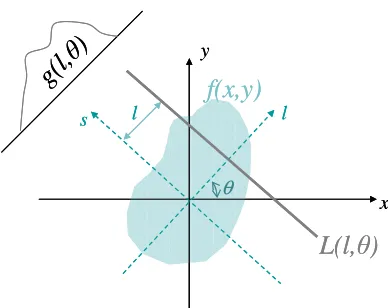
Figure 2.2. Illustration of the line integral geometry in a 2D plane.………11

Figure 2.3. A sinogram (left) of a simple object (right). The sinogram is formed by stacking projection data of the object taken from 0 to 180°.………..12

Figure 2.4. Illustration of the Fourier slice theorem: the 1D Fourier transform of the projection data is equal to the 2D Fourier transform of the image evaluated on the line that the integration g(l,θ) was calculated from.………..14

Figure 2.5: Possible system configurations of a micro-CT scanner. The panels from left to right show the cone beam, optical magnification, and Bragg diffraction based micro-CT scanner (Ritman, 2004; Robinson et al., 2005; Stampanoni et al., 2002a).………18

Figure 2.6: The schematic of a CNT x-ray tube. The single-wall carbon nanotubes (SWNTs) coated on a metal substrate were used as the cathode. The gate electrode is a metal mesh 50– 200 µm away from the cathode. Electron emission is triggered by the voltage applied between the gate and the cathode. X-ray is produced when the emitted electrons were accelerated and bombarded on the copper target. (Yue et al., 2002)………..23

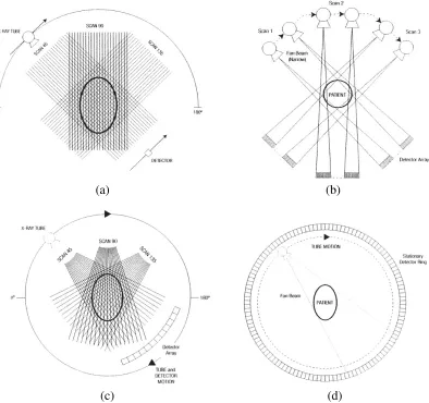
Figure 2.7. Four generations of incremental CT machines. (a) First generation linear and rotating pencil beam system; (b) linear and rotating fan beam system; (c) rotation only (tube and detectors) wide angle fan beam system; (d) fourth generation 360° detector ring-rotating tube system. (Dawson and Lees, 2001).………..25

Figure 2.8. Illustration of the spiral/helical CT scanning geometry. (Kalender, 2006).……..27

Figure 2.9: Schematic cross-section view of the electron beam CT scanner developed in UCSF (Robb et al., 1983; Peschmann et al., 1985)..………...28

(14)

Figure 2.11: Scanning geometries of the multiple sources CT scanner proposed by Berninger and Redington, with multiple rotatable detectors (left) or a fixed detector ring (right) (Berninger and Redington, 1980).………...30

Figure 2.12: Geometry of the dual-source CT system introduced by Siemens. (Flohr et al., 2006; McCollough et al., 2007)………...31

Figure 2.13: Illustration of four different choices for data collection in transmission tomography (Siltanen et al., 2003).………..32

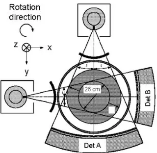
Figure 2.14. Principles of single-slice (a) and multi-slice (b) ECG-gated spiral scan (Kachelriess and Kalender, 1998; Flohr et al., 2005).……….42

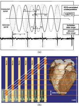
Figure 3.1. (a) The square geometry in the central transaxial plane. Two source arrays form two contiguous sides of a square, and two detectors form the other two sides. (b) The hexagonal geometry in the central transaxial plane. Three source arrays form three contiguous sides of the hexagon and three detectors form the other three sides. The imaging object is supposed to be at the center of the square/hexagon, within a 3.2 cm diameter mouse holder.………..53

Figure 3.2. Sinogram maps of the square geometry (left) and the hexagonal geometry (right). The shaded area represents the sampled points and the blank area gives the missing data. Each individual “diamond” corresponds to one source-detector pair. The vertical lines indicate the expected field of view.……….54

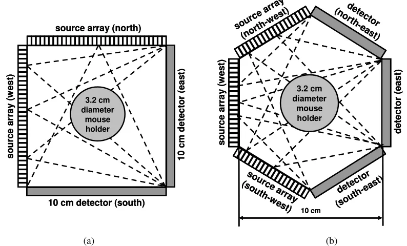
Figure 3.3. Illustrations of the phantoms used in the simulations. (a). The central axial (left) and transaxial (right) views from the multi-sphere phantom; (b). The central coronal (left), sagittal (middle), and transaxial (right) views of the MOBY phantom. The images are obtained from the filtered backprojection reconstructions from an ideal rotational CT.………...58

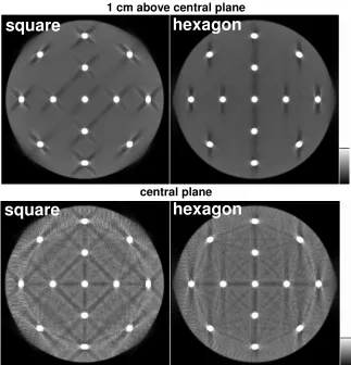
Figure 3.4. Transaxial slices from the reconstructions (saved at 5 iterations) of the multi-spheres phantom from the square (left column) and the hexagonal (right column) geometries. The axial locations of each set of slices are marked above the images………..62

Figure 3.5. Mean squared error in the uniform background regions in the reconstructions of the multisphere phantom from the square and the hexagonal geometries at different numbers of iterations. This is a quantitative measure of the error due to the limited-angle artifacts. The differences between the two geometries are marked beside each group of bars.………...63

(15)

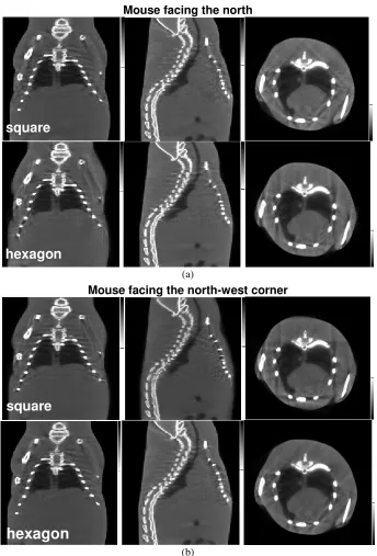
from left to right: the central coronal views, central sagittal views, and central transaxial views from the reconstructed images saved at 5 iterations.……….64

Figure 3.7. Mean squared error in the uniform background regions in the reconstructions of the MOBY phantom versus phantom orientations for the square and the hexagonal geometries. This is a measure of streaking artifacts due to limited-angle acquisition. The angle increments counter-clockwise. The data are obtained from 5 iterations..………..65

Figure 3.8. The axial FWHM of the PSF at the north-west location in each axial slice (a) and the average transaxial FWHM of the PSFs in the central axial slice (b) in the reconstructions from the square and the hexagonal geometries. The data are obtained from 5 Figure 3.9. The anisotropy of PSFs in the transaxial plane, 0.575 cm from the central plane. Data obtained from 5 iterations.………..67

Figure 3.10. The average variances at different regions in the central transaxial plane. Data obtained from 5 iterations………..68

Figure 3.11. The resolution-noise trade-off curves for the two geometries represented by the axial FWHM(a)/average transaxial FWHM(b) versus the average variance in the central region of FOV………69

Figure 4.1. Geometry of the proposed rotation-free micro-CT system. Two source arrays form two contiguous sides of a 10 cm square and two detectors form the other two sides. Each source array consists of 50 X-ray sources. The primary field of view is at the center, indicated by the “3.2 cm mouse holder”………...79

Figure 4.2. The percentage deviation of the OSC normalization images from the corresponding MOSC normalization image with regard to the number of updates (10 subsets per iteration) for an example reconstruction………...84

Figure 4.3. Coronal views (top row) and transverse views (bottom row) in the central plane from the reconstructions of the MOBY phantom with OSC and MOSC from (a) the 40keV

monochromatic spectrum and (b) the 40kVp Molybdenum polychromatic spectrum (both from 5 iterations). Dimensions of both reconstructions are 256×256×400 with a pixel size of 0.0125 cm. The coronal views only show the central 272 slices………..85

Figure 4.4. (a). Axial profiles (left) and transaxial profiles (right) from the polychromatic reconstructions with OSC and MOSC (both from 5 iterations). Locations of the profiles are marked in the inserted images. (b). Percentage difference images of the OSC and MOSC reconstructions that are shown in figure 4.3(b), displayed on a 0-20% scale. Left: coronal view; right: transverse view……….86

(16)

Figure 4.6. The average transaxial FWHM (left) and axial FWHM (right) of the PSF at the center of FOV in the monochromatic reconstructions with MOSC and OSC at 5, 10, 15 and 20

iterations……….87

Figure 4.7. The central transverse views from the reconstructions with MOSC and OSC from projections with simulated Poisson noise. Top: regular-noise (1×10-3 mAs per source); bottom: extremely-high-noise (1×10-6 mAs per source). The average variances (scaled by 106) calculated from 100 noise realizations for five different regions are marked on each image. All images and variance data shown are obtained from 5 iterations………...88

Figure 4.8. The average variance at soft tissue, bone, and lung regions in the variance images calculated from 100 noise realizations at regular-noise (top row) and extremely-high-noise (bottom row) situations………...89

Figure 4.9. The average variance versus average transverse FWHM curves (left column) and average variance versus axial FWHM (right column) at the center region of the FOV for MOSC and OSC at regular-noise (top row) and extremely-high-noise (bottom row) situations………...91

Figure 4.10. CPU time for reconstructing the system with OSC and MOSC at 5, 10, 15, and 20 iterations……….91

Figure 5.1. The proposed motion-free micro-CT system with square (left) and hexagonal (right) geometries (Quan and Lalush, 2005, 2007)………97

Figure 5.2. Schematics of the four groups of square geometries with various gaps between source arrays and detectors………..100

Figure 5.3. Schematics of the hexagonal geometries (right) and their corresponding square

geometries (left) with 10% gaps (top) and 20% gaps (bottom)………101

Figure 5.4. Sinogram maps of the square geometries with gaps. Left column: geometry a; right column: geometry b………..103

Figure 5.5. Percentage of missing data within 3cm FOV in the eight square geometries with gaps………...104

Figure 5.6. Sinogram maps of the hexagonal geometries (right) and their corresponding square geometries (left). (a) no gaps; (b) 10% gaps; (c) 20% gaps……….105

Figure 5.7. Illustrations of the phantoms used in the simulations. (a). The central axial (left) and transaxial (right) views from the multi-sphere phantom; (b). The central coronal (left), sagittal (middle), and transaxial (right) views of the MOBY phantom. The images are obtained from the filtered backprojection reconstructions from an ideal rotational CT………107

(17)

Figure 5.9. Central transaxial views from the reconstructions of the multi-sphere phantom from the square geometries with gaps. Images were obtained from 5 iterations………..112

Figure 5.10. Total MSE in the MSE images obtained from the four groups of geometries in comparison with the original, gap-free square geometry. Data obtained from 5 and 20 iterations are shown. The percentage increases of the total MSE for each geometry relative to the gap-free geometry are marked on the chart………113

Figure 5.11. Local MSE around each sphere in the mid-plane for the gap-free geometry and the geometry (a) in groups I-IV. The data were obtained from 5 iterations. The indices of the spheres are marked on the inserted image……….114

Figure 5.12. Anisotropy of the PSFs in the mid-plane for the square geometries with and without gaps. Data obtained from 5 iterations………...115

Figure 5.13. Resolution-noise tradeoff curves for the square geometries with and without gaps at five transaxial locations in the central plane………116

Figure 5.14. Central transaxial views from the reconstructions of the multi-sphere phantom from the hexagonal geometries and their corresponding square geometries………117

Figure 5.15. Comparison of the total MSE values in the MSE images for the square and

hexagonal geometries at 5 iterations………118

Figure 5.16. Resolution-noise tradeoff curves for the square and hexagonal geometries with and without gaps at five transaxial locations in the central plane………...119

Figure 6.1. Schematic drawings of the 4-row source module. (a) front view; (b) side view…...125

Figure 6.2. Schematic of the rotation-free micro-CT geometry (top view)……….126

Figure 6.3. Sinogram maps of the rotation-free micro-CT system with no-translation scanning (a) and bitranslation scanning (b)………..127

Figure 6.4. Illustration of the no-translation and bi-translation scanning modes of the rotation-free micro-CT system. The blue arrows indicate the source-detector pair involved in each

situation………129

Figure 6.5. Schematics of the finite focal spot sampling scheme. (a) samplings of the focal spot on the Gaussian profile in one-dimension; (b) front view of source-let distributions in two-dimension; (c) weighting factors for each source-let………...132

(18)

Figure 6.7. Reconstructions of the MOBY phantom from the rotation-free micro-CT system with notranslation and bi-translation scanning modes. (a) central Coronal views; (b) central Sagittal views; (c) central transaxial views………...138

Figure 6.8. Reconstructions of the multi-sphere phantom from the rotation-free micro-CT system with notranslation and bi-translation scanning modes. (a) central axial views; (b) central

transaxial views. Display grey scales were narrowed down to reveal details of artifacts………139

Figure 6.9. Local MSE measured around each spheres in the reconstructions of the multi-sphere phantom. (a) MSE variations within the mid-transaxial plane. Indices of the spheres are marked on the inserted image. (b) MSE variations of sphere No.1 at different axial locations…………140

Figure 6.10. Reconstructions of the uniform cylinder phantom with simulated compound Poisson noise. Average standard deviations at selected regions are overlaid on the images………141

Figure 6.11 Axial FWHM of the PSFs obtained with the no-translation and the bi-translation scanning modes under (a) infinitesimal and (b) finite (100 µm) focal spot situations…………144

Figure 6.12 Average transaxial FWHM of the PSFs obtained with the no-translation and the bi-translation scanning modes under (a) infinitesimal and (b) finite (100 µm) focal spot

situations………..145

Figure 6.13 Anisotropy of transaxial FWHM of the PSFs obtained with the no-translation and the bitranslation scanning modes under (a) infinitesimal and (b) finite (100 µm) focal spot

(19)

1 INTRODUCTION

The recent development of microfabricated X-ray sources using field emission from carbon nanotubes (CNT) instead of thermionic emission has opened up many new possibilities in development of specialized X-ray devices (Cheng et al., 2004; Zhang et al., 2005). These devices are capable of fast pulsing, modulation, and triggering from physiologic signals. Also, they can be microfabricated, leading to the possibility of creating imaging systems based on dense arrays of X-ray sources.

In this dissertation, such arrays of CNT-based x-ray sources are implemented into proposed designs of a fast, rotation-free micro-CT system; one of them is shown in figure 1.1. In this design, there are two fixed arrays of x-ray sources, with fifty sources each, spaced at 2 mm, and two 10 cm detectors arranged as shown. The primary field of view (FOV) of such a

3.2 cm diameter

mouse holder source array

s

our

c

e

a

rr

ay

10 c

m

det

ec

tor

10 cm detector

(20)

system is indicated by the “mouse holder” in the center of the square bounded by the source arrays and detectors. Tomographic angular sampling in this system is achieved by pulsing the individual sources one or more at a time, so that no rotation of the sources or subject is required. One of the key advantages of such a design is the high temporal resolution that it could achieve, which could be up to nano-seconds, as long as the detector frame rate is high enough. The stationary design also facilitates gated imaging and makes the system more reliable. Using ultra-short x-ray pulses, instead of continuous radiation, the system can also result in lower dose.

The proposed arrayed-source geometry, however, does not meet the conditions for full tomographic reconstruction; that is, it does not achieve a full 180-degree of angular sampling for every point in the field of view. For a 3cm FOV, over 10% of the complete data could be missing in an ideal geometry (Chapter 3) and over 20% for a more practical geometry (Chapters 5 and 6). Further, different points in the FOV have different arcs acquired. Thus, we expect that limited-angle artifacts will appear in the reconstructed images and the point spread functions in such a system will be spatially-variant and anisotropic. In this dissertation, the imaging properties of the proposed micro-CT system were studied by computer simulations.

(21)

compared to the square geometry. Therefore, it is expected to produce better image quality than the square geometry. The performances of the two geometries are compared in chapter 3 of this dissertation.

Gaps between the source arrays and the detectors are formed when there are ineffective margins on one or both ends of the source arrays or the detectors, which is inevitable in a real world realization of the proposed system. In chapter 5, a few sets of the square and the hexagonal geometries with various distributions and levels of gaps have been studied and the effect of gaps on the image quality is compared among the proposed geometries.

Further, a more practical design of the micro-CT system is studied in chapter 6, which has two multi-row source arrays and non-uniformly distributed gaps among the source arrays and detectors. A bi-translation scanning mode is proposed for this system, in which the imaging subject is translated to two other positions during the image acquisition in order to obtain additional angular coverage. Such a scanning mode of the system is compared to the case when the subject is stationary. In comparing the spatial resolution of the two scanning modes, both an infinitesimal and a finite x-ray source focal spot have been simulated.

(22)

computation time. The resulting new algorithm was named the modified OSC (MOSC). It was examined and compared to the OSC algorithm in the proposed rotation-free micro-CT system with the ideal square geometry.

The research presented here will show that the proposed micro-CT system can be effectively reconstructed using the OSC or the MOSC algorithm. The MOSC is up to 30% faster than the OSC and produces similar image quality. The ideal hexagonal geometry is superior to the square geometry in reducing limited-angle artifacts. However, it loses its advantages when gaps are introduced in the geometries. For either geometry, image quality degrades as the size of the gaps increases. We will also show that the scanning mode with subject translation is advantageous in reducing limited-angle artifacts while producing less isotropic point spread functions than the scanning mode with stationary subject.

References

Beekman F J and Kamphuis C 2001 Ordered subset reconstruction for x-ray CT Physics in Medicine and

Biology46 1835-44

Cheng Y, Zhang J, Lee Y Z, Gao B, Dike S, Lin W, Lu J P and Zhou O 2004 Dynamic radiography using a carbon-nanotube-based field-emission x-ray source Review of Scientific Instruments75 3264-7

Feldkamp L A, Davis L C and Kress J W 1984 Practical cone-beam algorithm Journal of the Optical Society of

America a-Optics Image Science and Vision1 612-9

Haimson J 1979 X-RAY SOURCE WITHOUT MOVING PARTS FOR ULTRAHIGH SPEED TOMOGRAPHY Ieee Transactions on Nuclear Science26 2857-61

Kamphuis C and Beekman F J 1998 Accelerated iterative transmission CT reconstruction using an ordered subsets convex algorithm Ieee Transactions on Medical Imaging17 1101-5

Lalush D S and Tsui B M W 2000 Fast transmission CT reconstruction for SPECT using a block-iterative algorithm Ieee Transactions on Nuclear Science47 1123-9

(23)

(24)

2 BACKGROUND

Over a century ago, the invention of x-ray opened up the door to medical imaging technologies. The “inner view” of a subject was generated for the first time under the exposure of x-ray radiation. Today, x-ray imaging, also called projection radiography, remains the most widely used imaging modality in medicine.

Radiographs – images generated from projection radiography – are essentially shadows cast by the semi-transparent imaging subject illuminated by x-rays. In other words, they are the projections of all features along the x-rays’ path, which, as a result, become overlapped in the image. There is no way to distinguish the overlapping features from a single radiograph without additional information on the anatomy. This means that projection radiography intrinsically loses depth information and is not capable of resolving features along the projection paths.

(25)

In this chapter, we first introduce the general principles behind x-ray CT technology. Next, we describe a category of x-ray CT that is specialized for small animal imaging, namely micro-CT. We then discuss in more detail a few aspects of x-ray CT that are most relevant to the scope of this study, including the x-ray sources, imaging geometries, reconstruction algorithms, and statistical models for x-ray CT. This chapter ends with a brief introduction to cardiac imaging, which is the assumed application of the micro-CT geometries proposed in this study.

2.1 General principles of x-ray Computed Tomography (CT)

X-ray CT produces cross-sectional images of the imaging subject based on a series of projection images taken around the subject from different angles. A typical x-ray CT system usually consists of a source that emits x-ray radiation, a detector for capturing the transmitted x-rays through the imaging subject, and a subject stage (a patient bed in the case of clinical CT). Most current x-ray CT systems utilize a rotational geometry – that is, either the subject stage or the source-detector gantry rotates around a fixed axis on a circular or helical orbit during the image acquisition. In this section, we will base our discussion on such a geometry; some of the non-traditional geometries will be discussed in section 2.4.

2.1.1 X-ray radiation patterns

(26)

x-ray radiation patterns, which can be largely divided into three categories: parallel-beam, fan-beam, and cone-beam.

The earliest x-ray CT scanners used parallel-beam radiation – they confine the x-ray into narrow, pencil-shaped beams and scan the object in parallel fashion, as shown in figure 2.1(a). Such a configuration is straightforward and convenient for implementing reconstruction algorithms; however, its drawbacks are obvious: the image acquisition is very time-consuming since a parallel-beam projection is formed by shifting the pencil-beam radiation in a parallel fashion within the transverse plane; besides, it only allows the reconstruction of a single 2D slice at a time.

A fan-beam x-ray, as shown in figure 2.1(b), is generated by restricting the x-ray radiation in the axial direction so that the beam forms the appearance of a fan on a 2D plane. The fan-beam geometry is much more efficient than parallel beam because the x-ray beam can fully cover the 2D cross-section of the object. Like parallel beam CT systems, early fan-beam CT systems used 1D detector arrays so that only a single cross-section image can be reconstructed at a time. Later, multi-slice fan-beam systems have been developed; they stack

x y z

(a) (b) (c)

(27)

multiple rows of 1D detector array along the axial direction so that multiple 1D projection can be captured at each rotation angle and multiple 2D slices can be reconstructed after each rotation.

Owing to the development of solid-state flat-panel detectors, the cone-beam radiation mode has emerged and the data acquisition became faster since then. Cone-beam radiation is an extension of fan-beam to the axial direction, the x-ray radiates from the point source divergently towards a 2D detector array, instead of a 1D detector array as in fan-beam case, forming a cone-shaped beam (figure 2.1(c)). This allows fan projections to be collected in a large axial range so that the projection data set of a 3D volume can be collected simultaneously, therefore the 3D volume can be reconstructed from a single scan, which substantially increases the imaging efficiency.

2.1.2 Acquisition of image signal

No matter which x-ray radiation pattern is used in the x-ray CT system, the detector response of an x-ray projection is the integration of transmitted x-ray beams long the x-ray paths. The detector intensity Id at any point of the detector always follows the basic equation

according to the fundamental photon attenuation law:

,

)

(

exp

0 

 



₋

_∫

=

I

s

ds

I

_d

µ

(2.1)

(28)

x-ray path. The integration

∫

µ(s)ds gives the total attenuation coefficient of the subject along the x-ray path.

To be precise, µ(s) is not only a function of spatial location, but also a function of the incident x-ray energy. Since the x-ray spectrum for CT is usually polychromatic, the detector response is actually the weighted integration over all the energy components of the x-ray beam (Lasio et al., 2007). In this case, the calculation would be much more complicated. Equation (2.1) has simplified the calculation by replacing the energy-dependent distribution of µ by that at the effective energy, which is defined as the energy that, in a given material, will produce the same measured intensity from a monochromatic source as is measured using the actual polychromatic source (Prince and Links, 2006). Hence, the images reconstructed from x-ray CT are approximately the distribution of linear attenuation coefficients at the effective energy of the polychromatic source.

Taking a log transform to the measured detector intensity Id in equation (2.1), we obtain

the following relationship:

.

)

(

ln

0

∫

=













−

=

s

ds

I

g

_d d

µ

(2.2)

Here, gdis usually called the projection data. Note that, after such processing, the projection

(29)

2.1.3 Radon transform and Sinogram

Let us rewrite the linear attenuation coefficient distribution as a function of rectangular coordinates in a 2D plane,µ(x,y). Consider a line integral through this object in this 2D plane with parallel x-ray beam; assume the line, L(l,θ), has distance l from the origin and angle θ with the x-axis, as illustrated in figure 2.2, then integration along this line, g(l,θ), can be written as:

(

cos

sin

)

.

)

,

(

)

,

(

∫ ∫

∞

∞ −

∞

−

+

−

=

x

y

x

y

l

dxdy

l

g

θ

µ

δ

θ

_(2.3)

The delta function in the above equation sifts the line L(l,

θ

) so that the integration is performed only along this line. The collection of g(l,θ) at all distance l and angle θ is called the 2D Radon transform of the function

µ

(x,y) . It relates the 2D distribution of linear attenuation coefficients to its projection data, and the inversion of the Radon transform produces the reconstruction of the 2D function.

x y

l s

θ

f(x,y)

l

g(

l,

θ

)

L(l,

θ

)

x y

l s

θ

f(x,y)

l

g(

l,

θ

)

L(l,

θ

)

(30)

The 2D Radon transform can be visualized as a 2D image, by stacking the individual 1D projection data from each angle sequentially. Such an image is called a sinogram. Figure 2.3 shows a simple object and its corresponding sinogram for 0 to 180° projection data. The horizontal axis of a sinogram represents the lateral location on the detector, while the vertical axis represents the projection angle.

2.1.4 Tomographic reconstruction

Now the question is, once we have a full collection of projection data, whether the 2D object function can be recovered or not. The answer is yes; and this fact is stated in the Fourier slice theorem, which relates the 1D projections of a 2D object and the 2D object itself in the Fourier domain. To derive this theorem, let us first take the 1D Fourier transform of the projection data with regard to the lateral distance l:

{

(

,

)

}

(

,

)

,

)

,

G(

₁_D

∫

∞ 2

∞ −

−

=

g

l

θ

g

l

θ

e

j πρl

dl

θ

ρ

F

_(2.4)

(31)

whereG(

ρ

,

θ

)denotes the Fourier transform of g(l,θ)with spatial frequency ρ. Now plug the expression of

g

(

l

,

θ

)

in equation (2.3) into above, and we get:

.

)

,

(

)

,

G(

∫ ∫

∞ 2 ( cos sin )

∞ − ∞ ∞ − + −

=

µ

x

y

e

j πρ x θ y θ

dx

dy

θ

ρ

_(2.5)

On the other hand, the 2D Fourier transform of the object functionµ(x,y)results:

{

}

_{∫ ∫}

∞ ∞ − ∞ ∞ − + −

=

(

,

)

(

,

)

.

)

,

(

u

v

₂_D

x

y

x

y

e

2 ( )

dx

dy

Μ

F

µ

j π xu yv _(2.6)

Observing the right hand side of equations (2.5) and (2.6) closely, we can easily find that they become the same if

) 7 . 2 (

sin

cos







=

θ

ρ

θ

ρ

v

u

is satisfied, which in turn results in the following relationship:

).

sin

,

cos

(

)

,

(

ρ

θ

M

ρ

θ

ρ

θ

G

=

_(2.8)

(32)

Although the Fourier slice theorem proved the invertibility of Radon transform and suggested a straightforward method for reconstructing the original image, this method is seldom used in practice due to several practical problems – it is impossible to obtain an infinite number of projections to form a complete 2D Fourier space; and it is difficult to interpolate the 1D Fourier transforms obtained on a polar coordinate system to a 2D rectangle coordinate system.

The most widely used method for x-ray CT reconstruction is filtered back-projection (FBP). Starting from the 2D inverse Fourier transform in polar coordinates, its derivation is straightforward and is shown below:

. ) , ( ) , ( 0 ) sin cos ( 2

∫ ∫

₋∞_∞ + = π

ρ

θ

πρ θ θ

ρ

θ

µ

x y M ej x y d d (2.9)

Equation (2.9) is the formula for the inverse Fourier transform calculation in polar coordinates(ρ,θ); the factorρ in the integral is the determinant of the Jacobian of the change

x y l s θ μ(x,y) g(l, θ) u v θ M(u,v)

1D Fourier transform 2D Fourier transform

x y l s θ μ(x,y) g(l, θ) u v θ M(u,v)

1D Fourier transform 2D Fourier transform

Spatial domain Fourier Domain

(33)

of variable from rectangular to polar coordinates. Then, the equation can be rearranged to the following form:

.

)

,

(

)

,

(

0 _cos _sin

2

∫ ∫

+ = ∞

∞

−









=

π

θ θ

πρ

_ρ

_θ

θ

ρ

µ

x

y

G

e

d

y x l l j

(2.10)

In the above equation, the term in the square bracket is the 1D inverse Fourier transform of the function ρG(ρ,θ), which can be considered as the projection dataG(ρ,θ)filtered by a high-pass filter, ρ . The filter is known as the ramp filter because of its appearance. The operation in the square bracket is usually called the “filtered back-projection” along angle θ; basically, it “smears” the projection data back to the image field along the line l. The final image is formed by integrating the “smeared” images at all angles.

The filtration operation in equation (2.10) is sometimes conducted in the spatial domain, where the multiplication of the projection data and the filter becomes a convolution operation. This form of FPB algorithm is also called convolution back-projection and it is written as below:

∫ ∫

₋∞_∞

+

−

=

π

θ

µ

0

(

,

)

(

cos

sin

)

,

(

x

y

g

l

c

x

y

l

dl

d

_{. (2.11)}

Functionc(x)in the above formula represents the inverse Fourier transform of the ramp filter. In practical implementations, c(x)has to be an approximation because the true ramp filter has no inverse Fourier transform.

(34)

Theoretically, projections obtained beyond this angle are redundant because they are the mirror images of the projections with an offset of 180°.

The parallel-beam FBP algorithm derived above can be easily adapted to fan-beam reconstruction, by transforming the parallel-beam parameter set to the fan-beam parameter set (Avinash C. Kak, 1988). Fan-beam geometries with circular detector (equiangular rays) and with planar detector (equidistance rays) result in different forms of reconstruction formulas, but both can be interpreted as weighted FBP algorithm. However, a 180° sampling arc would not be enough for fan-beam reconstruction any more. To guarantee that every point in the FOV is sampled over 180°, the source and detector has to rotate for another angle with is equal to the opening angle of the fan-beam (fan angle). Thus, the minimum rotation arc for fan-beam reconstruction is 180° plus fan angle.

Cone-beam reconstruction is a more complicated issue than parallel- and fan-beam reconstructions. The cone-beam acquisition with a single circular orbit does not allow exact reconstruction, because the 3D FOV cannot receive sufficient angular coverage, even over a full 360° rotation arc, except for the central plane where the rotation orbit lies. Tuy has found that to achieve a complete set of projection data for cone-beam reconstruction, a more complicated imaging geometry has to be satisfied, which is known as the Tuy’s completeness condition and it is stated as: “if on every plane that intersects the object there exists at least one cone-beam source (focal) point, then one can reconstruct the object.” (Tuy, 1983)

(35)

et al., 1984). This algorithm is based on the equidistance fan-beam FBP formula, which is extended to 3D space by treating the cone-beam x-ray as a combination of many tilted fan-beams with different angles.

A number of other analytic reconstruction algorithms have been proposed for x-ray CT reconstructions, but the FBP based methods introduced above are simple and efficient so that they have been dominating in most practical x-ray CT systems. However, these methods usually can not provide satisfactory performance when the noise influence in the system is high. Moreover, it is difficult to incorporate more complex imaging geometries and more elaborate physical models into these analytic methods. In these situations, iterative algorithms are usually used.

(36)

2.2 Micro-CT

Owing to the advances in genomics and cell biology, small animal models are developed to mimic various human diseases and they have proved to be valuable tools for the investigation of the underlying mechanisms of disease processes. They serve as the bridge between in vitro and in vivo studies for human diseases and potential treatments so that the efficacy of the human disease study is greatly increased. Medical imaging techniques play a crucial role in the small animal studies. Since most clinical imaging systems can not satisfy the resolution requirement for small animal imaging applications, specialized small animal imaging systems have been widely developed.

Micro-Computed Tomography (Micro-CT) is an emerging tool for small animal imaging because of its high spatial resolution, low cost and capability of 3D imaging. It has obtained wide-spread application in a variety of small animal research areas. Various micro-CT systems have been developed by a number of different research groups, according to the way that they achieve the magnification required for high resolution, current micro-CT scanners

(37)

usually fall into one of the three types of configurations (Ritman, 2004), as shown in figure 2.5.

Cone beam geometry, as shown in the left panel of figure 2.5, is the conventional way of achieving maginification, where a point source is used to project the subject to a larger area detector array (Ritman, 2004; Paulus et al., 2000; Flynn et al., 1994). With parallel x-ray sources, the magnification can be achieved by either using optic magnifier, such as a lens or a tapered fiber-optic coupling (middle panel) (Ritman, 2004; Stampanoni et al., 2002b), or using a Bragg interferometer to generate wavelength-specific diffraction (right panel) (Ritman, 2004; Robinson et al., 2005; Stampanoni et al., 2002a).

A micro-CT system is not simply the scale-down of a normal CT. Since the imaging subject for CT is much smaller in size than CT, the resolution requirement for micro-CT is hence increased to a much higher level. When we proportionally scale down the resolution level of an adult human CT image to a micro-CT image of a mouse, the voxel size should be decreased to the order of (30 ~ 100 µm)3 (the voxel size of an adult human CT image is of the order of 1 mm3) (Ritman, 2004). To achieve high spatial resolution that is required for a micro-CT scanner, a number of issues should be considered, including the scanner geometry discussed above, the x-ray source, the detector, etc.

(38)

However, it is noted that the maximum power that can be applied to a micro-focus x-ray source with a stationary target is limited by the rate at which the heat can be dissipated, and the heat dissipation is proportional to the focal spot size (Flynn et al., 1994; Whitaker, 1988). Flynn et al (Flynn et al., 1994; Whitaker, 1988) observed that the maximum power in Watts for a micro-focus x-ray source with a stationary target is approximately 0.88

4 .

1 f , where f is the focal spot size in µm. Thus, with smaller focal spot size, the x-ray output power, and hence x-ray flux, is limited by this relationship; higher flux can be achieved at the cost of larger focal spot size. Therefore, in real applications, the trade-off between these two factors should be balanced. The power limit is less a problem for CNT FE x-ray sources. It is reported by Liu et al. that a higher tube current can be achieved when operating at comparable level of anode voltage and focal spot size as in the thermionic x-ray sources (Liu

et al., 2006). More details on CNT x-ray tubes are introduced in section 2.3.

(39)

Compton scatter in the x-ray-tissue interactions, therefore allowing better contrast for different soft tissue types (Dowseth et al., 1998). However, only very limited SR generating facilities are available in the world, which prevents them from wide-spread applications in general research.

As far as the x-ray detection system is concerned, some bench-top micro-CT systems still use image intensifiers, which provide more rapid illumination of the imaging array and hence allow for more rapid scanning (Dowseth et al., 1998; Johnson et al., 1999), but more current systems employ a scintillator screen coupled to a charge-coupled device (CCD) (Castelli et al., 1994) either via an optical lens or fiber optics (Dowseth et al., 1998). The optical lens coupling is relatively less efficient than the fiber optic coupling but it is flexible for varying the magnification; on the other hand, the fiber optic coupling is much more efficient but the magnification is fixed.

With all the technical advances in micro-CT, it has become a more and more attractive imaging modality for a variety of researchers. It has been used in many studies to show and monitor bone structures under different disease conditions (Jones et al., 2007; Recker et al., 2007; Turnquist et al., 2007; Robinson et al., 2005). With the help of radiopaque indicators, such as iodine or barium, micro-CT systems can achieve high soft tissue contrast, which allows them to be widely used in the detection of diseases involved with soft tissue, such as lung tumors (Paulus et al., 2000; Kennel and Mirzadeh, 1998; Kennel et al., 1999a; Kennel

(40)

they can be used to determine the accumulation of certain type of molecules in the tissue sample to make a meaningful comparison between animals (Ritman, 2004).

2.3 CNT-based X-ray sources

Conventional x-ray tubes use thermionic emission (TE) to generate electron beams. In thermionic emission, the cathode, usually a tungsten filament, is heated to a very high temperature, e.g. above 1000 ~ 2000°C (Sugie et al., 2001; Yue et al., 2002), so that electrons can obtain high enough energy to escape from the material. However, with the development of x-ray imaging techniques, the intrinsic limitations of thermionic x-ray tubes become more and more apparent. In general, thermionic x-ray tubes have a slow response time (Yue et al., 2002), which limits their temporal resolution, especially for gated and dynamic imaging (Cheng et al., 2004; Zhang et al., 2005a); the electrons generated from TE are randomly distributed so that they can not be focused to a Gaussian distribution, which makes it difficult to reduce focal spot size and limits their imaging spatial resolution (Yue et al., 2002; Kawakita et al., 2006); thermionic tubes also have reduced service life because the hot cathodes usually get thinner and thinner over a long duration through the sublimation of oxides (Sugie et al., 2001; Yue et al., 2002). Besides, the high operating temperature of thermionic x-ray tubes requires an additional power supply for heating, which makes them large in size and increases power consumption (Sugie et al., 2001; Yue et al., 2002).

(41)

Kawakita et al., 2006; Liu et al., 2006; Cheng et al., 2004). Unlike TE tubes, FE tubes use a cold cathode to generate electrons and their output current is voltage controllable (Sugie et al., 2001; Yue et al., 2002); CNTs are more stable and robust than metal materials (Sugie et al., 2001; Yue et al., 2002) and are found to be promising field emitters (Bonard et al., 1999; Collins and Zettl, 1997; Nilsson et al., 2000; Saito et al., 1999; Wang et al., 1998b). The schematic of a CNT x-ray tube is shown in figure 2.6 (Yue et al., 2002). CNT x-ray tubes possess a number of advantages over conventional TE tubes. They have an instantaneous response time so that they can generate x-ray radiation with significantly high temporal resolution of up to nano-seconds (Cheng et al., 2004). The low divergence of field emitted electrons and the Gaussian-distributed x-ray intensity generated from FE tubes result in better spatial resolution (Cheng et al., 2004) – the effective spatial resolution of a CNT based micro-Computed Tomography (CT) system is shown to be less than 30 µ m (Sugie et al., 2001; Yue

(42)

et al., 2002; Nicolaescu et al., 2002; Zhang et al., 2005a; Zhang et al., 2005b; Kawakita et al., 2006; Liu et al., 2006; Cheng et al., 2004). Operating at room temperature, the cold cathode of CNT tubes are much more stable than hot cathodes, which allows them to have much longer life time. Without the additional power supply for heating, CNT tubes have the potential to be constructed as compact, portable imaging devices (Sugie et al., 2001).

CNT x-ray tubes have shown their potential in various imaging applications. Several groups have obtained high quality x-ray radiography with CNT tubes for industrial or biological objects (Sugie et al., 2001). Cheng et al have generated short pulses of x-ray radiation with durations of milliseconds using CNT tubes and applied them for x-ray radiography of fast moving objects or for gated imaging of live objects (Cheng et al., 2004). Well-resolved images obtained from their works show great potential for dynamic imaging using CNT tubes. Zhang et al developed a multi-beam field emission x-ray source (MBFEX) by making use of the compact size of CNT field emitters; from the tomosynthesis reconstruction of an object with overlapped planes, different layers can be clearly identified (Zhang et al., 2005b). Later, Lalush et al obtained better tomosynthesis images with higher quality by improving the reconstruction algorithms for MBFEX (Lalush et al., 2006a; Lalush

(43)

2.4 X-ray CT imaging geometries

2.4.1 Rotation based CT geometries with single source

The imaging geometries of CT scanners have been changing over the years. Most of the scanners achieve their angular sampling based on circular rotation with a single x-ray source.

(a) (b)

(c) (d)

(44)

Depending on their source and detector configurations and the required motions, they largely fall into several generations, as illustrated in figure 2.7.

The first generation, which was also the earliest design, of CT scanners used a single-cell detector and a source that was collimated to produce a narrow, pencil beam radiation and was aligned with the detector. The lateral projections were sampled by linearly translating the source-detector pair across the subject, which resulted in a parallel-beam projection. Upon the completion of one projection set, the source-detector pair was rotated to the next angle and the lateral sampling was repeated.

The imaging geometry of the second generation scanners was similar to the first generation, except that a wider x-ray beam and multiple detector cells were used. In this design, multiple projection rays with different angles could be captured at the same time at each position, so that the same angular sampling of the subject could be achieved with fewer rotations. Thus, the scan time can be substantially reduced.

The third generation scanners brought another significant improvement in scanning efficiency by removing the translational motion that was used in the first and the second generation scanners. They employed a wide array of detector cells, which, together with the fan-beam x-ray radiation, covered the entire 2D cross-section of the subject such that allowed the simultaneous measurement of the fan-beam projection of the subject. Thus, the only motion necessary to this design was the rotation of the source-detector gantry. Today, most CT scanners used in clinic are based on the third generation scanner geometry.

(45)

rotational detector array by a ring-shaped detector encircling the subject, so that the detector can be kept stationary during the image acquisition. The source was mounted inside the detector ring and was the only rotating part in the geometry. Simultaneous fan-beam projections were also acquired in these scanners. Thus, compared with the third generation scanners, the fourth generation canners maintained similar imaging speed with reduced motion, and therefore lower system complexity. On the other hand, since the ring-shaped detector required a larger acceptance angle, the fourth generation scanners have a major drawback that they are more sensitive to scattered radiation.

With a single circular rotating orbit, the CT scanners described above are only able to collect the projection data for a single cross-sectional slice from a single 360° rotation. In order to obtain the projection data of other slices, the rotational scanning has to be stopped, the subject translated along the axial direction, and then the scanning restarted at the new position, namely the “step-and-shoot” fashion. The invention of spiral/helical CT has completely changed this situation. With spiral/helical scanners, the source and detector keep

(46)

the same rotation movement as the four generations of CT scanners described above; during the source/detector rotation, the subject is continuously translated along the axial direction of the subject, which results in a spiral/helical trajectory of the source relative to the subject, as illustrated in figure 2.8. Such geometry enabled continuous collection of 3D volumetric data without slowdown of the rotation movement, which greatly speeds up the imaging process of 3D volumes.

2.4.2 Rotation-free and multi-source CT geometries

Through the development of the x-ray CT scanner, there have existed several motion-free, or arrayed-source systems that resemble the geometries proposed in this dissertation. One of them is the electron beam CT (EBCT) scanner, which was originally motivated for ultra-fast scanning for dynamic cardiovascular imaging. EBCT was first developed in 1979 at the University of California at San Francisco (UCSF) (Boyd et al., 1979) and brought to medical applications by the Mayo clinic (Breen et al., 1992; McCollough et al., 1995). Unlike conventional CT, EBCT does not use a rotational x-ray tube; instead, it uses a specially

Figure 2.9: Schematic cross-section view of the electron beam CT scanner developed in UCSF (Robb

(47)

designed x-ray tube which has a large, ring-shaped anode and x-rays are generated by sweeping the electron beam, within the vacuum tube, through the anode ring. A schematic of the EBCT system is shown in figure 2.9. In a EBCT scanner, the four target rings lie in the gantry below the patient and the electron beam is bent electromagnetically onto one of the four target rings (Peschmann et al., 1985; Suetens, 2002; Boyd et al., 1979; Haimson, 1979). Each sweep of the target ring requires 50 ms, with 8-ms delay to reset the beam (Peschmann

et al., 1985; Suetens, 2002; Boyd et al., 1979; Haimson, 1979).

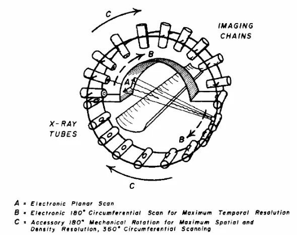
The dynamic spatial reconstructor (DSR), developed in 1983 at Mayo clinic, was also designed for ultrafast cardiac imaging (Robb et al., 1983). Similar to our design, DSR employes an array of x-ray tubes (consisting of 14 tubes), aligned along a semi-circle with very large diameter; the detectors, including a fluorescent screen and 14 video imaging

(48)

systems, are attached to the opposite semi-circle, as shown in figure 2.10. To achieve high temporal resolution reconstructions, the entire scanner is kept stationary and the x-ray tubes are pulsed one by one rapidly to obtain fast angular sampling. The scanner can also be rotated mechanically over a limited angle in order to achieve better spatial resolution (Robb

et al., 1983).

Although both of the two CT scanners have achieved certain degrees of success in dynamic cardiac imaging, they are not widely used today. Two significant drawbacks of both of them are their vastly larger size and much higher cost than conventional CT scanners.

The idea of employing multiple x-ray sources in a CT scanner has also been proposed elsewhere even earlier than the introduction of DSR, although with a rotational, instead of a stationary, scanning mode. In a patent published in 1980, Berninger and Redington described “a multiple source, rotating, tomographic x-ray scanner” (Berninger and Redington, 1980), in which a plurality of x-ray sources are employed. The sources can be arranged either along

(49)

the axial direction of the subject to improve the axial coverage, or within a transaxial plane to reduce the scanning time of a single slice, so that improve the temporal resolution. In conjunction with the multiple sources, such a system can either use multiple rotatable detector arrays, each opposite to one of the sources, or use a fixed detector ring. The number of sources typically chosen was 3, 5, or 7; the geometries with 3 sources are shown in figure 2.11.

Only in recent years, such a rotational, multi-source CT geometry was realized in commercial scanners. Siemens introduced a dual-source CT (DSCT) scanner equipped with two x-ray sources and two corresponding detectors (Flohr et al., 2006; McCollough et al., 2007). The two sets of source-detector pairs are mounted, with an angular offset of 90°, on a rotating gantry, as shown in figure 2.12. Since the two sets of source-detector pairs can acquire projection data simultaneously, the total scanning time for a fixed volume is reduced to roughly half of a single source system, so that the temporal resolution can be improved by a factor of 2. Further improvement in temporal resolution may be achieved by employing

(50)

three or more sources in the system, but with a cost that may prevent them from widespread applications (Wang et al., 2008).

2.5 Reconstruction algorithms for x-ray CT

2.5.1 Limited-angle problem

Generally, Computed Tomography (CT) uses projection data obtained from all around an object to reconstruct the cross-section structure of the object. However, in some applications, such as in dental radiology, surgical imaging, thorax imaging and mammography (Rantala et al., 2006), only a few projection images are taken. In some situations, the few projections are taken sparsely, but all around the object, which is called “sparse full angle data”; in some other situations, the few projections are taken from a limited angle of view, which is called “limited-angle data”; also, there is the “sparse limited-angle data” situation, as illustrated in figure 2.13 (Siltanen et al., 2003). The motion-free, linear-array source micro-CT system that proposed in this dissertation belongs to the “limited-angle data” case.

Because of the lack of information in the projection data, the reconstruction of a limited-angle system is an ill-posed problem (Rangayyan et al., 1985). For such cases, standard

(51)

data reconstruction algorithms, such as filtered backprojection (FBP), do not work well any more and they usually produce severe artifacts in the reconstructions (Rangayyan et al., 1985; Delaney and Bresler, 1998; Hanson and Wecksung, 1983; Hebert and Leahy, 1989; Lange, 1990; Siltanen et al., 2003). A number of different reconstruction algorithms have been designed for the limited-angle problem; most of them use an iterative method. Based on the reconstruction model used, here we divide the iterative algorithms into two categories: non-statistical methods and non-statistical methods.

2.5.2 Non-statistical reconstruction algorithms

(52)

augmented with the estimated projections form a consistent data set (Nassi et al., 1982; Ollinger, 1990).

The constraint Fourier reconstruction (CFR) algorithm is one of the representative Fourier space methods. Similarly with the IRR algorithm, it estimates the missing projection data by imposing a constraint, but the constraint is applied in the Fourier space (Fujieda et al., 1990; Karp et al., 1988). Compared with IRR, CFR is a more practical approach; also, it provides better convergence and requires less computation, especially for geometries with a large gap (Fujieda et al., 1990; Karp et al., 1988). There are many other algorithms that are based on the same idea of completing the missing data before reconstruction and their details can be found in (Kudo and Saito, 1991; Prince and Willsky, 1990; Soumekh, 1986).

A significant drawback of this type of method is that, through the process of estimating the missing data, no additional information is introduced; however, errors tend to accumulate at each stage of the iterative procedure. Furthermore, the convergence mechanism of these algorithms is not well defined (Andersen, 1989).

(53)

Another totally different type of reconstruction method is the projection onto convex sets (POCS). POCS is an iterative signal recovery algorithm and can be used in a wide variety of applications. Generally, it finds a solution that is consistent with available data and prior constraints. Allowable constraints imposed by data and prior knowledge are those that can be associated with convex sets; and the unknown signal must lie in the intersection of all the constraint sets (Peng and Stark, 1989; Kudo and Saito, 1991; Youla and Webb, 1982).

2.5.3 Statistical reconstruction algorithms

(54)

contrast for low-count data (Beekman and Kamphuis, 2001; Gilland et al., 2000; Manglos, 1992; Wang et al., 1998a).

The earliest statistical reconstruction algorithm is the ML-EM (or EM), which was originally designed for emission computed tomography (Shepp and Vardi, 1982; Lange and Carson, 1984) and was later adapted by Lange and Carson for transmission CT (Shepp and Vardi, 1982; Lange and Carson, 1984). However, the computational cost of the transmission version of EM algorithm is too high for most applications because it involves the calculation of a large number of line integrals of short segments (Lange and Fessler, 1995). Instead, a more popular type of statistical reconstruction algorithm for transmission CT is the Bayesian based method, which incorporates extra information into the statistical model used in the reconstruction (Hanson and Wecksung, 1983; Hebert and Leahy, 1989; Lange, 1990; Siltanen et al., 2003; Green, 1990).

(55)

fields (MRF) priors (Dobson and Santosa, 1996), etc. Each of these priors has its advantages and drawbacks, and may be successful for certain applications. A detailed review of the principles and performances of the priors can be found in (Siltanen et al., 2003).

Among these, Lange and Fessler developed a convex algorithm, which employed a Gibbs smoothing prior to the MAP estimation (Lange and Fessler, 1995). The convex algorithm resembles the EM algorithm but they showed that it is considerably more efficient than EM (Lange and Fessler, 1995). Later, the efficiency of the convex algorithm was further increased to a much higher level by using ordered subsets of projection data (Hudson and Larkin, 1994), and the resulting algorithm is called the ordered subsets convex (OSC) (Beekman and Kamphuis, 2001; Kamphuis and Beekman, 1998). A similar algorithm, the block-iterative transmission (BIT), was developed by Lalush and Tsui (Lalush and Tsui, 2000). They showed that BIT produces nearly identical results as OSC with a savings in processing time (Lalush and Tsui, 2000). In our applications, these two algorithms are implemented in the proposed imaging systems and their performances will be discussed in section 4.

2.6 Statistical model for x-ray CT

Imaging properties of a rotation-free, arrayed-source micro-computed tomography system

ABSTRACT