Electronic Thesis and Dissertation Repository
4-22-2014 12:00 AM
The hydrodynamic behavior of an inverse liquid-solid circulating
The hydrodynamic behavior of an inverse liquid-solid circulating
fluidized bed
fluidized bed
Amin Jaberi
The University of Western Ontario
Supervisor Jesse Zhu
The University of Western Ontario
Graduate Program in Chemical and Biochemical Engineering
A thesis submitted in partial fulfillment of the requirements for the degree in Master of Engineering Science
© Amin Jaberi 2014
Follow this and additional works at: https://ir.lib.uwo.ca/etd
Part of the Complex Fluids Commons
Recommended Citation Recommended Citation
Jaberi, Amin, "The hydrodynamic behavior of an inverse liquid-solid circulating fluidized bed" (2014). Electronic Thesis and Dissertation Repository. 1989.
https://ir.lib.uwo.ca/etd/1989
This Dissertation/Thesis is brought to you for free and open access by Scholarship@Western. It has been accepted for inclusion in Electronic Thesis and Dissertation Repository by an authorized administrator of
(Thesis format: Integrated Article)
by
Amin Jaberi
Graduate Program in Chemical and Biochemical Engineering
A thesis submitted in partial fulfillment of the requirements for the degree of
Master of Engineering Science
The School of Graduate and Postdoctoral Studies The University of Western Ontario
London, Ontario, Canada
ii
Abstract
In this work the hydrodynamic behavior of an inverse liquid-solid circulating fluidized bed
(ILSCFB) system was studied. In addition, the hydrodynamic characteristic of the inverse
liquid-solid fluidization under the conventional fluidization regime was also studied. The
system consists of a downer with an inner column diameter of 7.6 cm and a height of 5.4
meters, an upcomer (riser) with an inner column diameter of 20 cm, a separator, and feeding
and returning pipes which connect the downer and the upcomer. Based on the axial
hydrodynamic behavior of the ILSCFB, it was found that the axial solids holdup in the
downer is uniform. Similar to the heavy-particle LSCFB, the circulating fluidization regime
in the downer was separated into the two zones including the initial circulating fluidization
zone and the fully developed circulating fluidized zone as a function of the total liquid
velocity in the downer. The effects of the solids inventory and the counter current flow in the
upcomer on the hydrodynamics of the downer were also studied. Afterwards, the radial
distribution of particles was studied in the downer of the ILSCFB. Interestingly, the radial
structure of the two-phase flow was completely different from the case of the heavy-particle
LSCFB. It was found that the solids holdup was greater in the center than near the wall of the
downer. Finally, the conventional (non-circulating) inverse liquid-solid fluidization was
studied in a column with a large diameter for the first time. The minimum fluidization
velocity was obtained experimentally and compared with the Richardson and Zaki model. It
was concluded that the Richardson and Zaki model can predict the bed expansion in the case
of the inverse liquid-solid fluidization when the terminal velocity was calculated by the
model of free rising light particles.
Keywords
Inverse liquid-solid circulating fluidized bed (ILSCFB), axial solids holdup, solids
circulation rate, liquid velocity, radial distribution of particles, conventional fluidization
iii
Acknowledgments
I would like to express my gratitude and appreciation to all those who gave me the possibility
to complete this report.
I take this opportunity to express my profound gratitude and deep regards to my supervisor
Professor Jesse Zhu for his exemplary guidance, monitoring and constant encouragement
throughout the course of this thesis. The blessing, help and guidance given by him time to
time shall carry me a long way in the journey of life on which I am about to embark.
The completion of this project could not have been accomplished without the support of my
co-supervisor, Professor Dimitre Karamanev. I offer my sincere appreciation for the learning
opportunities provided by him.
Special thanks go to support staff members of our group Jianzhang Wen and Hanning Li to
help me to modify and design the experimental equipment. In addition, many thanks to
George Zhang for his service
Last but not least, many thanks go to Tian Nan who helped me to carry out the experiments
and gave suggestion in different parts.
Thanks are also extended to my friends, Ha Doan, Chengxiu Wang, Long Song,
Vahid Vajihinejad, Cristina Salome Lugo, Stanislav Ivanov, Arash Mozaffari and Hojat
Seyedy, who have always been helping and supporting me in the academic and daily life.
iv
Co-Authorship Statement
Title: The Axial Hydrodynamic Behavior of Light Particles in an Inverse Liquid-Solid Circulating Fluidized Bed
Author: Amin Jaberi, Jesse Zhu, Dimitre Karamanev
All the experiments were carried out by Amin Jaberi under the gaudiness of the advisors Jesse Zhu and Dimitre Karamanev. All drafts of this manuscript were written by Amin Jaberi. Modifications were completed under the supervision of advisors Jesse Zhu and Dimitre Karamanev. The final version of this manuscript is ready for submission.
Title: Radial Distribution of Light Particles in an Inverse Liquid-Solid Circulating Fluidized Bed
Author: Amin Jaberi, Dimitre Karamanev, Jesse Zhu, Tian Nan
v
Table of Contents
Abstract ... ii
Acknowledgments... iii
Co-Authorship Statement... iv
List of Tables ... viii
List of Figures ... ix
List of Appendices ... xii
Chapter 1 ... 1
1 General Introduction ... 1
1.1 Introduction ... 1
1.2 Objectives ... 3
1.3 ThesisStructures ... 3
References ... 5
Chapter 2 ... 7
2 Experimental Apparatus and Measurement Techniques ... 7
2.1 Inverse liquid-solid circulating fluidized bed ... 7
2.2 Measurement techniques ... 9
2.2.1 Solids circulation measuring device ... 9
2.2.2 Manometers... 10
2.2.3 Optical fiber probe ... 15
2.2.4 Electrical resistance tomography ... 16
Nomenclature ... 18
References ... 20
Chapter 3 ... 21
vi
3.2 Materials and Methods ... 23
3.3 Results and Discussion ... 24
3.4 Conclusion ... 35
Nomenclature ... 35
References ... 36
Chapter 4 ... 38
4 Radial distribution of light particles in an Inverse Liquid-Solid Circulating Fluidized Bed ... 38
4.1 Introduction ... 38
4.2 Material and Methods ... 40
4.3 Results and Discussion ... 42
4.4 Conclusions ... 50
Nomenclature ... 51
References ... 52
Chapter 5 ... 54
5 Hydrodynamic characteristics of inverse liquid-solid fluidization in a large column . 54 5.1 Introduction ... 54
5.2 Mathematical models of bed expansion and the minimum fluidization velocity correlation ... 55
5.2.1 Richardson and Zaki model ... 55
5.2.2 The minimum fluidization velocity ... 57
5.3 Experimental Setup ... 57
5.4 Results and discussions ... 58
5.5 Conclusion ... 62
Nomenclature ... 62
vii
Chapter 6 ... 66
6 Conclusions and Recommendations ... 66
6.1 Conclusions ... 66
6.2 Recommendations ... 67
Appendices ... 68
AppendixA: Operation of the ERT………...…....68
viii
List of Tables
Table 2-1: Positions of the pressure ports on the axial direction ... 10
Table 5-1: The minimum fluidization velocity obtained by mathematical models and
ix
List of Figures
Figure 1-1: Left: upward fluidization, Right: downward (inverse) fluidization ... 1
Figure 2-1: Schematic diagram of the inverse LSCFB reactor (Sang [1]) ... 8
Figure 2-2: Schematic diagram for the measurement of the average solids holdup ... 11
Figure 2-3: Schematic diagram for the measurement of the frictional bed pressure drop ... 13
Figure 2-4: Schematic diagram for the measurement of the bed expansion ... 14
Figure 2-5: The optical fiber probe diagram for solids holdup measurement (Razzak et al. [4]) ... 16
Figure 2-6: Schematic diagram of ERT (Razzak et al. [4]) ... 17
Figure 3-1: Schematic diagram of the inverse LSCFB reactor designed by Sang [19] ... 24
Figure 3-2: Variation of (A) the superficial solids velocity and (B) the average solids holdup versus the superficial liquid velocity at different auxiliary liquid velocities in the downer ... 26
Figure 3-3: Variation of the average solids holdup versus the superficial liquid velocity at different superficial solids velocities in the downer ... 28
Figure 3-4: Variation of the axial solids holdup distribution under the circulating fluidization regime ... 30
Figure 3-5: Effect of solids inventory in the upcomer on (A) the superficial solids velocity and (B) the average solids holdup in the downer at auxiliary liquid velocity of Ua = 2.78 cm/s ... 31
x
different conditions (Ur = 0 cm/s and Ur = 0.4 cm/s) at superficial solids
velocity of Us = 1.4 cm/s ... 34
Figure 4-1: Schematic diagram of the inverse LSCFB reactor designed by Sang [15] ... 41
Figure 4-2: Radial distribution of the solids holdup obtained by OFP based on the
comparison of the probe movement at superficial liquid velocity of Ul = 40.4
cm/s and height of 2.1 meters below the distributor ... 43
Figure 4-3: Radial distribution of the solids holdup obtained by OFP at auxiliary velocity of
Ua = 5.6 cm/s and (A) height of 2.1 meters (B) height of 3.4 meters below the distributor ... 44
Figure 4-4: Radial distribution of the solids holdup obtained by both ERT and OFP under the
two different superficial velocities at auxiliary velocity of Ua = 2.8 cm/s ... 45
Figure 4-5: Radial distribution of the solids (glass beads) holdup using both ERT and optical
fiber probe under different superficial liquid velocities at auxiliary liquid
velocity of 1.4 cm/s (Razzak et al. [18]) ... 46
Figure 4-6: Three dimensional topographic view of the cross-sectional solid holdup at
superficial liquid velocity of Ul = 33.4 cm/s and superficial solids velocity of
Us = 1.5 cm/s ... 48
Figure 4-7: Two-dimensional topography view from 0.5s to 10s frame cross-sectional solids
holdup at superficial liquid velocity of Ul = 33.4 cm/s and superficial solids
velocity of Us = 1.5 cm/s ... 50
Figure 5-1: Schematic diagram of the inverse LSFB reactor designed by Sang [15]... 58
Figure 5-2: Variation of (A) the frictional bed pressure drop (B) the dimensionless height
versus the superficial liquid velocity in the upcomer ... 60
Figure A-1: Variation of the solids holdup versus time at the superficial liquid velocity of
xi
by both ERT and manometers when for each measurement by the ERT σm was
obtained, but data was processed by the first value of σl measured at the last
step of the calibration ... 68
Figure A-2: Variation of the solids holdup versus time at the superficial liquid velocity of
Ul = 22.3 cm/s and the superficial solids velocity of Us = 0.52 cm/s obtained by both ERT and manometers when for each measurement σm and σl were
obtained ... 69
Figure B-1: Error bars for radial solid holdup……….………70
xii
List of Appendices
Appendix A: Operation of the ERT ... 68
Appendix B: An example of error bars for solid holdup………...………….70
Chapter 1
1
General Introduction
1.1 Introduction
Inverse/upward liquid-solid fluidization refers to a two-phase system where particles with
density lower/higher than liquid density are suspended by a stream of liquid flowing in
the opposite direction to buoyancy/gravity. In upward liquid-solid systems, particles
density is higher than liquid density. Thus, the fixed bed of particles at the bottom of the
fluidized column is fluidized when an upward liquid stream is uniformly distributed into
the fixed bed. Therefore, the drag force counters the gravitational force at liquid velocity
beyond the minimum fluidization velocity of particles. In contrast, when the density of
particles is lower than the liquid density, particles tend to stay at the top of the fluidized
column. In this case, fluidization is obtained by a downward flow of the liquid and
consequently drag force counters the buoyancy force at liquid velocity beyond the
minimum fluidization velocity.
In a downward or inverse fluidization, at a liquid velocity below the minimum
fluidization velocity, particles remain in a fixed state at the top of the fluidized column
known as the downer. When liquid velocity increases beyond the minimum fluidization
velocity, the fluidization of particles is obtained and the liquid-solid system enters the
conventional fluidization regime. In this regime of fluidization, there is a clear boundary
between the dense region of the particles at the top and the bottom freeboard which is
occupied by liquid [1]. Further increasing the liquid flowrate in the downer causes this
clear boundary to disappear and a more dilute mass of particles in the liquid is observed.
By further increasing the liquid velocity beyond the terminal rising velocity, particles are
transported out of the column [2, 3]. Under this condition, particles are carried out of the
downer by the downward liquid stream. If particles are separated at the bottom of the
downer and stored in another column, particles recirculation can be achieved between the
two columns by continuously feeding particles to the top of the downer from the second
column.
This idea resulted in designing the novel two-phase system named "Inverse Liquid-Solid
Circulating Fluidized Bed", by Sang [4].
Generally fluidized bed reactors known as dense fluidized bed reactors have been used in
a wide range of applications. Interestingly, in the case of liquid-solid fluidization, some
biotechnological processes such as an aerobic wastewater treatment [5, 6], and ferrous
iron oxidation [7] in inverse fluidized bed biofilm reactors have demonstrated that inverse
fluidized bed bioreactors are more efficient in comparison to upflow fluidized bed
reactors. In addition, studies about the hydrodynamic behavior of the inverse liquid-solid
fluidization for example hydrodynamic characteristics of inverse liquid-solid fluidization
[8], bed expansion of inverse liquid-solid fluidization [9], and Newton’s law for free
rising spheres [10] have shown that in some parts hydrodynamic behavior of the inverse
liquid-solid fluidization is different from the upward one and further research in this area
is still necessary.
On the other hand, it was found that a type of fluidized bed reactor, circulating fluidized
bed (CFB), has more advantages rather than dense phase fluidized bed reactors [1]. It was
concluded that operation of the CFB at high velocity increases the contact between the
particles and the fluid [1]. On this basis, application of upward liquid-solid circulating
as waste water treatment [11] and continuous recovery of proteins from unclarified whole
broth [12].
In the last two decades, comprehensive hydrodynamic studies of upward LSCFB reactors
for instance radial distribution of particles [13], radial distribution of the liquid velocity
[14], axial hydrodynamic behavior of the LSCFB [2], and the onset velocity of the
LSCFB [15] have been carried out. These works can set a proper pattern to study the
hydrodynamic behavior of the inverse liquid-solid circulating fluidized bed.
1.2 Objectives
The primary steps to understand capabilities of the inverse liquid-solid circulating
fluidized bed reactor are to study the hydrodynamic behavior of this reactor. On this
basis, the main objectives of this work are
1- To conduct a study on the axial hydrodynamic of the inverse LSCFB including
solids circulation rate and particles distribution in the downer.
2- To observe the effects of some factors such as solids inventory and counter
current flow in the riser or upcomer on solids circulation rate and particles
distribution in the downer.
3- To employ the proper techniques to measure the radial phase distribution.
4- To study the radial flow structure in the downer under the circulating fluidization
regime.
5- To compare the hydrodynamic behavior of the inverse and upward LSCFB.
6- To investigate the inverse liquid-solid fluidization under the conventional
fluidization regime in a column with a large diameter.
1.3 Thesis
Structures
Based on the objectives, this thesis includes the following chapters:
Chapter 1 contains a simple definition of the upward and inverse liquid-solid fluidization
Chapter 2 describes the experimental setup and different techniques of measurements
applied in this study.
Chapter 3 reports the axial hydrodynamic behavior of the inverse LSCFB. In this chapter,
the solids circulation rate and the average solids holdup under a wide range of operating
conditions in the downer are discussed and compared to the results for the upward
LSCFB. Later, the effects of different factors such as solids inventory and counter current
flow in the riser or upcomer on the downer hydrodynamics are studied.
Chapter 4 shows the results of the experimental study of the radial flow structure of the
inverse LSCFB. Three measurement techniques were employed and the current results
are compared with previous results obtained for the upward LSCFB reactor containing
particles with density higher than liquid density.
Chapter 5 presents the results of the study of the pressure drop and bed expansion in the
riser or upcomer with a larger diameter. The minimum fluidization velocity is measured
and different equations are presented to predict the minimum fluidization velocity.
Chapter 6 summarizes the conclusions obtained in the above studies and gives
References
[1] Zhu, J.-X., D. G. Karamanev, A. S. Bassi and Y. Zheng (2000). "(Gas-) liquid-solid circulating fluidized beds and their potential applications to bioreactor engineering". The Canadian Journal of Chemical Engineering 78(1): 82-94.
[2] Zheng, Y., J.-X. Zhu, J. Wen, S. A. Martin, A. S. Bassi and A. Margaritis (1999). "The axial hydrodynamic behavior in a liquid-solid circulating fluidized bed". Canadian Journal of Chemical Engineering 51(50): 16242-16250
[3] Liang, W., S. Zhang, J.-X. Zhu, Y. Jin, Z. Yu and Z. Wang (1997). "Flow characteristics of the liquid-solid circulating fluidized bed". Powder Technology 90(2): 95-102.
[4] Long Sang (2013). "Particle Fluidization in Upward and Inverse Liquid-Solid Circulating Fluidized Bed". The University of Western Ontario, PhD Thesis.
[5] Nikolov, L., D. Karamanev, T. Penev, and D. Dimitrov (1990). "Full-Scale Inverse Fluidized Bed Biofilm Reactor for Wastewater Treatment" 2nd Int. Biotechnol. Conf.: Asian-Pacific Biotechnol. Conf., 112, Seoul, Korea.
[6] Karamanev, D. G. and L. N. Nikolov (1996). "Application of inverse fluidization in wastewater treatment: From laboratory to full-scale bioreactor". Environmental Progress 15(3): 194-196.
[7] Karamanev, D. G., and L. N. Nikolov (1988). "Influence of Some Physicochemical Parameters on Bacterial Activity of Biofilm". Biotechnol. Bioeng. 31(4): 295-299
[8] Fan, L.-S., K. Muroyama and S. H. Chern (1982). "Hydrodynamic Characteristics of Inverse Fluidization in Liquid-Solid and Gas-Liquid-Solid Systems". The Chemical Engineering Journal 24(2): 143-150.
[9] Karamanev, D.G., Nikolov, L.N., (1992b). "Bed expansion of liquid–solid inverse fluidization". AICHE Journal 38(12): 1916-1922
[10] Karamanev, D.G., Nikolov, L.N., (1992a). "Free rising spheres do not obey Newton’s law for free settling". AICHE Journal 38 (11), 1843–1846.
[11] Chowdhury, N., J. Zhu, G. Nakhla, A. Patel and M. Islam (2009). "A novel liquid-solid circulating fluidized-bed bioreactor for biological nutrient removal from municipal wastewater". Chemical Engineering and Technology 32(3): 364-372.
[13] Razzak, S. A., S. Barghi, J.-X. Zhu (2009). "Application of electrical resistance tomography on liquid–solid two-phase flow characterization in an LSCFB riser". Chemical Engineering Science 64(12): 2851-2858
[14] Zheng, Y., Zhu, J.-X. (2003). "Radial distribution of liquid velocity in a liquid–solid circulating fluidized bed". International Journal of Chemical Reactor Engineering 1, Article Number: S1.
[15] Zheng, Y. and J.-X. Zhu (2001). "The onset velocity of a liquid-solid circulating
Chapter 2
2
Experimental Apparatus and Measurement Techniques
2.1 Inverse liquid-solid circulating fluidized bed
A schematic diagram of the inverse liquid-solid circulating fluidized bed (ILSCFB)
reactor used in this study is shown in Figure 2-1. The reactor downer was operated at a
liquid superficial velocity higher than the particle terminal rising velocity. Therefore, it is
essential to feed particles at the top of the downer and to separate the entrained particles
from its bottom and recirculate them back to the top of the downer again.
The reactor consists of a Plexiglas downer with an inner column diameter of 7.6 cm and a
height of 5.4 meters, a Plexiglas liquid-solid separator, a Plexiglas riser or upcomer with
a diameter of 20 cm, and the solids return and feed pipe connecting the downer and
upcomer. In this study, the solid phase was represented by spherical Styrofoam spheres
with a mean diameter of 0.8 mm and density of 28 kg/m while liquid phase was tap
water. The density of the particles was measured with the fully automatic and accurate
gas displacement pycnometer, "AccuPyc 1340".
At the top of the downer, main and auxiliary liquid distributors are installed to introduce
the water into the downer. The main liquid distributor was made of seven stainless steel
tubes occupying 19.5% of the downer area and extended 0.2 m down from the column
top, and the auxiliary liquid distributor was made of a porous plate with 4.8% opening
area at the top of the downer. The system also included two water tanks connected to
each other as the source of the water for the entire system. From one tank water is
pumped and divided into two streams leading to the main and auxiliary liquid
Figure 2-1: Schematic diagram of the inverse LSCFB reactor
(Sang [1])
When the total liquid velocity in the downer reaches the minimum fluidization velocity,
particles move away from each other and the bed of the particles from the fix bed
expands slowly in a downward direction. With a further increase of the superficial liquid
velocity over the terminal velocity, particles begin to move out of the bed. Under this
condition, particles are carried by the downward liquid flow and then at the bottom of the
downer are separated from the liquid in a cylindrical liquid–solid separator. Liquid is
returned to the liquid tank through the pipe which was designed as a Π - shape. The
maximum height of this pipe is at the highest level of the reactor to ensure that the entire
system is filled with water during the experiments. On the other hand, particles move
from the separator to the upcomer through the pipe which connects the separator and
the top of the upcomer. Then through the pipe connected from the top of the upcomer,
particles feed into the top of the downer and recirculation of the particles completes in the
reactor. The auxiliary liquid flow plays an important role in controlling the circulation of
the particles. If auxiliary flow is set on zero, circulation of the particles is no longer
occurring.
Periodically, water inside the tanks was refilled to prevent the accumulation of external
substances which influence the hydrodynamic measurement. The temperature of the
water was checked during experiments to make sure that all the experiments were
performed under the same condition.
2.2 Measurement techniques
2.2.1
Solids circulation measuring device
In order to measure the superficial solids velocity in the downer, a devise named the
solids circulation measuring device [2] was located near the bottom of the upcomer. The
upcomer was divided into two equal sections with two half butterfly valves mounted at
the top and the bottom of the two-half section. By properly flipping the two half butterfly
valves from one side to the other, particles moving up in the upcomer can be accumulated
on one side of the measuring section and increased further in the form of packed bed. A
certain distance from the top of the valve where particles begin to accumulate is marked.
Thus, the required time to fill that volume with particles is measured and the superficial
solids velocity is calculated by the following equation:
=
(#$)ɛ% (2.1)
where &' and &( are the areas of the upcomer and downer respectively, ℎ is the
accumulated height of particles in the measuring section and * is the accumulation time
2.2.2
Manometers
In this study, manometers were used to measure the average solids holdup, pressure drop
across the bed and bed expansion. Six ports at different heights were placed along both
the downer and the upcomer. These ports were connected by tubes to a series of
manometers. Table 2-1 shows the exact place of the pressure ports along both columns.
Since the hydrostatic pressure at different heights of both columns was high, open-end
manometers were not used in this experiment to prevent the overflowing of water in
manometers. In this case, the ends of the manometers were connected to a tank full of air
and the pressure of air inside the tank was controlled.
Table 2-1: Positions of the pressure ports on the axial direction
Distance from main liquid distributor (cm)
Downer (7.6 cm I.D.)
Distance from liquid distributor (cm)
Upcomer (20 cm I.D.)
111.4 8.4
187.4 37.9
238.4 73.4
289.4 109.4
366.4 144.4
416.4 179.4
Average solids holdup
As long as downer or upcomer is occupied only by water, the level of water inside the
manometers was equal. Before each test, this level was checked to make sure that
pressure ports were not blocked by particles or bubbles of air. But if the downer or
water was lower than water density inside the manometers, water levels inside the
manometers were different. Between the two manometers the pressure balance is
governed by the following equation:
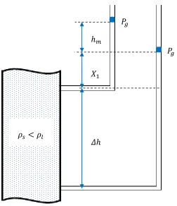
+,+ ./ℎ01 + ./123+ 4./(1 − ɛ) + .ɛ617ℎ − ./17ℎ − ./123− +, = 0 (2.2)
By simplification of Equation (2.2), average solids holdup is obtained by the following
equation:
ɛ
=
89
×
;<;<=;
(2.3)
where ℎ0 is the height difference between the levels of the water inside the manometers,
7ℎ is the distance between the pressure ports, ./ and . are the liquid and the particles density respectively.
Figure 2-2: Schematic diagram for the measurement of the average solids holdup
. < ./
ℎ0
23
7ℎ
+,
Pressure drop across the bed
One of the common ways to find the minimum fluidization velocity is to measure the
pressure drop across the bed.
7+?@A( = 7+@A(− BC./1 (2.4)
Based on Equation (2.4), the frictional bed pressure drop depends on the total pressure
drop across the bed and the pressure due to the height of the fluid. In the case of gas-solid
fluidization, the second term is negligible because the density of the gas is small. On this
basis, it is assumed that in gas-solid fluidization the frictional bed pressure drop is equal
to the total pressure drop across the bed. However, in liquid-solid fluidization the second
term is not negligible because the liquid density (in this study water) is high.
In order to find the pressure drop across the bed, one port was located close to the
distributor. Another port was located at low enough height of the upcomer to ensure that
the bed expansion of particles no longer reaches to this height. The pressure in points 1
and 3 is obtained by the following equations with manometers:
+3 = 23./1 + ℎ0./1 + +, (2.5)
+ = 23./1 + BC./1 + 2D./1++, (2.6)
On the other hand, the pressure difference between points 1 and 3 inside the column is
calculated by Equation (2.7):
+− +3 = 7+@A(+ 2D./1 (2.7)
By combination of Equations (2.5), (2.6) and (2.7), the total pressure drop across the bed
is calculated by Equation (2.8):
7+@A( = BC./1 − ℎ0./1 (2.8)
Based on the definition of the frictional bed pressure drop in Equation (2.4), 7+?@A( is
7+?@A( = ℎ0./1 (2.9)
Figure 2-3: Schematic diagram for the measurement of
the frictional bed pressure drop
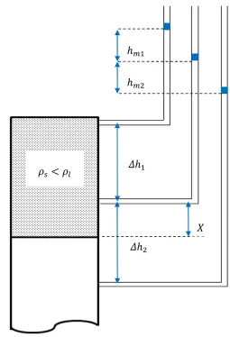
Bed expansion
One way to measure the bed expansion during the fluidization is to observe the variation
of the bed height versus the superficial liquid velocity visually. However, due to the
fluctuation of particles at the bottom of the bed, this kind of measurement is not easy and
accurate. Another way to measure the bed expansion is to measure it based on the
variation of the pressure drop across the bed of particles.
+,
+,
ℎ0
23
2D
BC
. < ./
+
Firstly, the average solids holdup at the section of the column occupied by both particles
and water (Figure 2-4) is defined by the following equation:
ɛ
=
98EE
×
;<
;<=;
(2.10)
Since the fluidized bed is in the conventional fluidization regime and particles are
dispersed homogeneously in both radial and axial directions, solids holdup is constant in
the entire bed. In this case, the bed expansion is obtained by the following equation:
2 =
8ɛ
×
;<;<=;
(2.11)
Figure 2-4: Schematic diagram for the measurement of the bed expansion
ℎ03
ℎ0D
7ℎ3
7ℎD
2.2.3
Optical fiber probe
In order to measure the local solids holdup, an optical fiber probe (OFP) containing a
multitude of light transmitting fibers was used. The model of the probe was PV-5
manufactured by the Institute of Process Engineering, Chinese Academy of Sciences. The
tip of the probe is circular with a diameter of 3.8 mm. This area includes approximately
8000 emitting and receiving quartz fibers. These fibers are arranged arbitrarily and the
diameter of each fiber is 15 µm. In a simple expression, emitting fibers transfer the light
from the source of the light to the measuring volume. Depending on the concentration of
particles, the scattered light is reflected and conducted by the receiving fibers. The light is
then diverted at the beam splitter and consequently transformed and amplified to the
output voltage ranging from 0 to 5. Then, using an Analog/Digital converter the output
voltage signal is fed to a personal computer.
The small size of the probe does not totally disturb the flow structure. This measuring
device is not expensive and complicated. In addition, some problems such as
temperature, humidity, electromagnetic fields and electrostatics do not influence the
measurements [3].
The output of the optical fiber system is a voltage signal. It was calibrated precisely
before each experiment. One of the best methods of calibration of the optical fiber probe
was described by H. Zhang et al. [3]. Although in their study the optical fiber probe was
used in a gas-solid fluidized bed, some procedures were also useful in a liquid-solid
fluidized system. One of the procedures applied in this study was the use of two black
boxes. One of the black boxes was full of particles and another one was empty. Before
the main calibration, these two boxes were used to set the appropriate range for the zero
Figure 2-5: The optical fiber probe diagram for solids holdup measurement
(Razzak et al. [4])
For each test, the calibration of the optical fiber probe was carried out on site. In this
study, the calibration of the optical fiber probe was performed in the circulating
fluidization regime. At the height of the downer in which the optical fiber probe
measured the voltage, average solids holdup was measured by the two manometers as
well. Thus, at different flowrates of liquid in the downer, several measurements were
obtained by the optical fiber probe and the manometers. By using the relation between
the solids holdup and electrical voltage, a linear relationship for the calibration of the
optical fiber probe was obtained. During each experiment, the average solids holdup was
measured by the manometers to ensure the accuracy of the optical fiber probe.
2.2.4
Electrical resistance tomography
Recently, a non-intrusive system of measurement named electrical resistance tomography
(ERT) was introduced for the experimental research of multiphase flow. This system can
measure the local phase distributions by electrical resistivity measurements of the
multiphase flow. The system used in this study was manufactured by the En'Urga Inc.
The ERT consists of sixteen conductivity sensors equally spaced around its wall, an
electronic circuit and a PC-based data acquisition system. The inner diameter of ERT was
built equal to the inner diameter of the downer to line up the sensors with the wall of the
downer. ERT has the ability to acquire data at 250 frames per second. Based on the
frame, multiple driving currents are sequentially fed into a pair of neighboring electrodes.
With the applied current source, electrical potential distributions are generated within the
fluids and the wall. Electronic circuits sense voltages and currents between the electrodes
and send them to a PC-based data acquisition system. Using the values of electrical
potentials and currents, the local electrical conductivity of the liquid-solid mixture can be
calculated and then reconstructed through a state-of-the-art optimization algorithm to
provide the phase distributions. The conductivity distribution is converted into the solids
holdup based on Maxwell’s relation shown in Equation (2.12):
ɛ
=
DF<=DF8DF<GF8
(2.12)
where H/ is the conductivity of continuous phase and H0 is the conductivity of the
mixture. The main concept behind the Maxwell`s equation is that the continuous phase of
the mixture (in the present study water) should be electrically conductive and the second
phase (Styrofoam bead) should include equal-sized spheres that are not electrically
conductive [5].
Riser Wall Electrode Cross-section of ERT
ERT Sensor
Data Acquisition System
Image Reconstruction System
Current Signal Voltage Signal
Figure 2-6: Schematic diagram of ERT (Razzak et al. [4])
Similarly to the calibration of the optical fiber probe, the ERT calibration was carried out
accurate data. In this work, M 541P compact precision conductivity meter was used to
perform conductivity measurements quickly and reliably.
As shown in the structure of the inverse LSCFB, the system includes two water tanks
connected to each other. Water is pumped from one tank and introduced to the downer
and the upcomer. The second tank was designed to gather water from both columns.
During the calibration of the ERT, the conductivity of water increased from 300 µ Si/cm
to around 1400 µ Si/cm in seven or eight steps. In each step, 30 grams of table- salt was
added to the first tank and water was circulated through the entire system (downer and
upcomer). Then the conductivity of water in both tanks was measured. If the conductivity
of water in both tanks was equal to each other, it was assumed that the conductivity of
water in the entire system was the same. At this given conductivity, the ERT was run to
take one second of data while only single phase liquid flowed through the test section.
This collected data was treated and saved by a program made in I + +.
This step was repeated to increase the conductivity of water to around 1400 µ Si/cm.
During several experiments, it was found that if the number of steps was higher than six,
the accuracy of the calibration and consequently results obtained by ERT in each test was
high. At the final step of the calibration, data processing was done in the Matlab
Environment and polynomial curve fitting was applied to obtain the calibration curve.
The program showed an error regarding the best function which can fit the data. If the
error was less than 1%, the accuracy of the results during the experiment was agreeable.
Nomenclature
&' Cross sectional area of the upcomer (riser) (JD)
&( Cross sectional area of the downer (JD)
BK Solids inventory height (J)
ℎ0 Height difference between the levels of water inside the manometers (J)
ℎ Accumulated height of particles in measuring section (J)
* Accumulation time of particles in the measuring section (M)
Superficial solids velocity (J/M)
N Auxiliary liquid velocity (solids-free basis) – downer (J/M)
/ Total liquid velocity (solids-free basis) – downer (J/M)
Greek Letters
./ Density of the liquid (O1/J)
. Density of the solids (O1/J)
ɛ Solids holdup
7ℎ Distance between the pressure ports (J)
7+@A( The total bed pressure drop (+L)
7+?@A( The frictional bed pressure drop (+L)
σP The conductivity of the liquid (QRS/TJ)
σU The conductivity of the mixture (liquid and particles) (QRS/TJ)
References
[1] Long Sang (2013). "Particle Fluidization in Upward and Inverse Liquid-Solid Circulating Fluidized Bed". The University of Western Ontario, PhD Thesis.
[2] Zhu, J.-X., D. G. Karamanev, A. S. Bassi and Y. Zheng (2000). “(Gas-) liquid-solid circulating fluidized beds and their potential applications to bioreactor engineering". The Canadian Journal of Chemical Engineering 78(1): 82-94.
[3] Zhang, H., P. M. Johnston, J. X. Zhu, H. I. de Lasa and M. A. Bergougnou (1998). "A novel calibration procedure for a fiber optic solids concentration probe". Powder Technology 100(2-3): 260-272.
[4] Razzak, S. A., S. Barghi, J.-X. Zhu (2009). "Application of electrical resistance tomography on liquid–solid two-phase flow characterization in an LSCFB riser". Chemical Engineering Science 64(12): 2851-2858
Chapter 3
3
The axial hydrodynamic behavior of light particles in
an Inverse Liquid-Solid Circulating Fluidized Bed
3.1 Introduction
Inverse liquid-solid fluidization refers to a two-phase system where solid particles with
density lower than liquid density are suspended by a stream of liquid flowing in the
opposite direction to buoyancy. In the inverse liquid-solid fluidization, by increasing the
stream of liquid and reaching the minimum fluidization velocity, particles move away
from each other and the bed of the particles expands slowly in a downward direction
from the boundary of the fix bed. This kind of fluidization regime is named conventional
inverse fluidization where there is a clear boundary between the dense region of particles
in the top and the bottom freeboard which is occupied by liquid [1].
The advantages and the applications of the inverse liquid-solid conventional fluidized
reactors have been shown in last two decades. In the area of the biotechnology, Nikolov
and Karamanev [2] found that a bioreactor working under these conditions would be able
to control the biofilm thickness. Thus, the application of this bioreactor was described in
different reports for such applications as anaerobic digestion of distillery effluent [3] and
biological aerobic wastewater treatment [4, 5]. The previous reports on the
hydrodynamics of inverse liquid-solid conventional fluidization showed that the
hydrodynamics of inverse liquid-solid fluidization is different from that of an upward
one. Fan et al. [6] used experimental bed expansion data to modify the Richardson and
Zaki model in terms of Reynolds number, Archimedes number and liquid holdup.
Karamanev and Nikolov [7] found that the Richardson and Zaki model predicted their
experimental data for particles of different characteristics agreeably when the terminal
velocity was calculated by the model of free rising particles proposed by them [8].
Ulaganathan and Krishnaiah [9] studied a semi-fluidized regime before complete
fluidization. They proposed empirical correlations for the bed expansion in the
numbers, and liquid-solid density difference. Renganathan and Krishnaiah [10] studied
the voidage fluctuations, axial voidage profile and bed expansion. They proposed an
explicit correlation for the terminal velocity of a free rising particle.
When particles with density lower than the density of the liquid are fluidized in a column
known as a downer, particles begin to be transported out of the bed after reaching the
liquid velocity of the critical transient point [1]. Under this condition, particles are carried
out of the column by the downward liquid. If particles are separated at the bottom of the
downer and stored in another column, particle recirculation can be achieved between two
columns by continuously feeding the particles to the top of the downer. Under these
conditions, the boundary between the two phases is not clear in the downer and particles
are dispersed in the entire column. Generally for the upward liquid-solid fluidization, it
was shown that liquid-solid fluidized bed reactors working in the circulating fluidizing
regime have certain advantages compared to the reactors working under the conventional
fluidizing regime. Therefore, liquid-solid circulating fluidized bed reactors have been
used in different areas of chemical engineering. In the field of waste water treatment,
excellent lab-scale results led to the establishment of a pilot scale liquid-solid circulating
fluidized bed for the municipal wastewater treatment [11]. In the area of continuous ion
exchange processes, the application of liquid-solid circulating fluidized bed has resulted
in successful continuous protein recovery [12]. Regarding the biochemical production,
Patel et al. [13] introduced a novel liquid-solid circulating fluidized bed bioreactor for the
fermentative production of lactic acid. In the bio-refining processes, Trivedi et al. [14]
used a liquid-solid circulating fluidized bed as a continuous reactor for polymerization of
phenol.
The study of the hydrodynamic behavior of LSCFB reactors is important for determining
the capabilities of these reactors. In contrast to the inverse LSCFB, the hydrodynamic
behavior of upward liquid-solid circulating fluidized beds have been well documented.
The axial hydrodynamics of the liquid-solid circulating fluidized bed including the
variation of the axial phase distribution with varying solids circulation rate was studied
by Zheng et al. [15]. In that study, the effects of different factors such as solids inventory
stability of liquid-solid circulating fluidized bed was reported in a study by Zheng and
Zhu [16]. The demarcation of conventional fluidization regime from the circulating
fluidization regime and empirical relation to measure the critical velocity when
circulation of particles begins are important in the hydrodynamic study. Liang et al. [17]
proposed a regime map for the operation of the liquid-solid upward fluidization including
the conventional fluidization, circulating fluidization and transport regimes. In
comparison with the relation offered by Liang et al. [17], Zheng and Zhu [18] proposed
an onset velocity correlation for liquid-solid circulating fluidized bed ignoring the effects
of geometry of the system.
Recently, by combining the concepts of inverse liquid-solid fluidization and of
circulating fluidization, a novel type of two-phase system, "Inverse Liquid-Solid
Circulating Fluidized Bed", was proposed by Sang [19]. The aim of the current work is to
study the hydrodynamic behavior of this novel two-phase system containing particles
with density lower than the liquid density. Firstly, some experiments were conducted to
compare the results from the present two-phase system with the previous results which
had been obtained for the upward LSCFB. Then the solids inventory in the upcomer was
increased to observe its effect on the solids circulation rate and the average solids holdup
in the downer under the new conditions. Finally, a liquid stream was introduced from the
top of the upcomer to study its effect on the downer hydrodynamics where solids
circulation rate and average solids holdup were measured and compared with results in
which flowrate of the liquid in the upcomer was zero.
3.2 Materials and Methods
A schematic diagram of the inverse liquid-solid circulating fluidized bed (ILSCFB)
reactor used in this study is shown in Figure 3-1. The main parts and the operation of this
system were discussed in chapter 2.
The solids circulation rate and the superficial liquid velocity were measured by solids
circulation measuring device. This device was located at the bottom of the upcomer. Six
manometers. By measuring the pressure drop, the average solids holdup is obtained in the
downer.
The solid phase was represented by spherical Styrofoam beads with a mean diameter of
0.8 mm and a density of 28 kg/m while the liquid phase was tap water. All experiments were performed at ambient temperature.
Figure 3-1: Schematic diagram of the inverse LSCFB reactor designed
by Sang [19]
3.3 Results and Discussion
Circulating fluidization regime in the downer is obtained when the total liquid velocity in
this column is higher than the terminal rising velocity of particles. Continuous feeding of
stream introduced into the downer from the auxiliary distributor mobilizes the particles
transported from the solids feed pipe to the downer and accumulated between the main
and auxiliary distributor. Thus, once the particles reach the front of the main distributor,
they are carried by the main liquid stream in downward direction. If the auxiliary
flowrate is set at zero, the particles stay in the area between the auxiliary distributor and
main distributor, hence the circulation of particles is no longer occurring.
Through the solids feed pipe, the particles are transported to the top of the downer slowly
in a packed state. A minor portion of the auxiliary liquid stream flowing into the solids
feed pipe helps to reduce the friction between the particles and the wall.
The first set of the experiments was performed under the condition where the total solids
inventory in the upcomer was 0.9 meters (when all the particles are stored in the
upcomer). Figure 3-2-A shows the variation of the superficial solids velocity versus the
superficial liquid velocity at four different auxiliary liquid velocities. It is obvious that at
a fixed auxiliary liquid velocity, superficial solids velocity increased in the downer with
increasing the total liquid velocity. In addition, higher auxiliary flowrate resulted in
higher superficial solids velocity at a given total liquid velocity.
Similarly to the results reported by Zheng et al. [15] for the upward LSCFB, two distinct
zones during the circulating fluidization regimes were observed for the inverse LSCFB.
After the onset of the circulation, by increasing the superficial liquid velocity, the
superficial solids velocity increased sharply. This zone was referred to the initial
circulating fluidization zone [1]. However, after reaching a certain point, the superficial
liquid velocity did not increase significantly as the superficial solids velocity increased
further. In this case, the transition from the initial circulating fluidization zone to the
developed circulating fluidized zone was obtained.
Figure 3-2: Variation of (A) the superficial solids velocity and (B) the average solids
holdup versus the superficial liquid velocity at different auxiliary liquid velocities in
the downer 0 0.3 0.6 0.9 1.2 1.5
5 10 15 20 25 30 35 40
S upe rf ic ia l S ol ids V el oc it y ( cm /s
) Ua = 1.39 cm/s
Ua = 2.78 cm/s
Ua = 4.17 cm/s
Ua = 5.54 cm/s
(A)
0.02 0.04 0.06 0.08 0.105 10 15 20 25 30 35 40
A ve ra g e S ol ids H ol dup
Superficial Liquid Velocity (cm/s)
Ua = 1.39 cm/s Ua = 2.78 cm/s Ua = 4.17 cm/s Ua = 5.54 cm/s
At low auxiliary flowrates, the existence of the developed circulating fluidized zone was
observed when the solids circulation rate increased insignificantly with the increase of the
total liquid velocity. However, at high auxiliary liquid velocities, the increase of
superficial solids velocity with increasing the superficial liquid velocity continued
considerably even at high liquid velocities and the developed circulating fluidized zone
was not obtained in the downer. In the previous study by Zheng et al. [15] for the upward
LSCFB, it was proposed that at high auxiliary flowrates, the stable operating range
decreased in comparison to lower auxiliary flowrates. Similar behavior was also observed
in the inverse liquid-solid circulating fluidized bed as well. For instance, at auxiliary
liquid velocity of N = 2.78 TJ/M, the circulation of particles started at lower superficial
liquid velocity without facing the risk of unstable operation and the system was operated
in higher superficial liquid velocities as well. In contrast, at auxiliary liquid velocity
of N = 5.54 TJ/M, the circulation of the particles commenced at total liquid velocity of
/ = 16.7 TJ/M and before that the system faced an unstable operation and no
circulation of the particles was achieved in the system. In addition, it was observed that
the developed fluidization zone was not obtained at high superficial liquid velocities and
the further increasing of the superficial liquid velocity was not possible because of the
pump capacity limitation.
Figure 3-2-B shows the variation of the average solids holdup versus the superficial
liquid velocity at four auxiliary liquid velocities in the downer. Based on Figure 3-2, at
different auxiliary liquid velocities, higher auxiliary flowrate led to feeding more
particles and thus to higher average solids holdup in the downer.
At a fixed auxiliary flowrate, the average solids holdup in the downer decreased as the
superficial liquid velocity was increased. This trend is completely similar to the previous
results for the riser of the upward LSCFB. In previous results reported by Zheng et al.
[15] and Liang et al. [17], it was concluded that increasing the superficial liquid velocity
can result in increasing the particles velocity and decreasing the residence time of the
particles in the riser which was observed in the current results for the downer of the
Two different zones including the initial circulating fluidization and developed
circulating fluidized zones are evident from Figure 3-2-B. At the beginning of the
circulation, the average solids holdup in the downer decreased quickly. After reaching a
certain velocity by further increasing the superficial liquid velocity, the average solids
holdup decreased slowly in the downer. This can be explained based on Figure 3-2-A
where the variation of the superficial solids velocities at higher superficial liquid
velocities was insignificant and the regime of the two-phase flow in the downer was at
the developed circulating fluidized zone.
Looking at Figure 3-3, it is clear that at higher superficial solids velocities, due to feeding
more particles into the downer, higher average solids holdup was obtained at a total
liquid velocity in the downer. In addition, at a fixed superficial solids velocity, the
increase in the superficial liquid velocity led to the decrease of the average solids holdup.
Such decrease was more evident at lower superficial liquid velocities, but with further
increasing the superficial liquid velocity, the average solids holdup in the downer
decreased slowly.
Figure 3-3: Variation of the average solids holdup versus the superficial liquid
velocity at different superficial solids velocities in the downer
0.02 0.04 0.06 0.08 0.10
5 10 15 20 25 30 35
A ve ra g e S ol ids H ol dup
Superficial Liquid Velocity (cm/s) Us = 0.48 cm/s
Us = 0.64 cm/s
One hydrodynamic advantage of the inverse LSCFB is related to the uniform distribution
of particles in the axial direction. The variation of the axial solids holdup under the
circulating fluidization regime is shown in Figure 3-4. In order to observe the axial solids
holdup in the downer at two different zones marked in Figure 3-2, two different liquid
velocities were chosen. When the superficial liquid velocity was high in the downer
(/ = 33.39 TJ/M) and the regime of circulating fluidization was in the developed
circulating fluidized zone, uniform axial average solids holdup was observed in the
downer. In addition, even when the superficial liquid velocity was low (/= 16.7 TJ/M)
in the downer and the regime of the circulating fluidization was still in the initial
circulating fluidization zone, axial solids holdup was observed to be uniform.
In the previous study of the upflow LSCFB by Zheng et al. [15] for lighter particles such
as plastic (. = 1100 O1/J) and glass (. = 2490W,
0X) beads, uniform distribution of the particles was observed in both zones. When heavier particles (steel shots with . =
7000 O1/J) were used, the axial solids holdup was non-uniform in the initial
circulating fluidization zone, but uniform at developed circulating fluidized zone [15]. It
is reasonable to assume that the density difference influences the distribution of particles
in the axial direction. When the density difference was large (.− ./ = 6000W,
0X for steel shots) the non-uniformity of particles distribution was observed, but at low density
differences (.− ./ = 100W,
0X for plastic beads and .− ./ = 1490
W,
0X for glass beads) a
uniform distribution of the particles was found in the upward LSCFB. On this basis, it
can be expected that since the density difference cannot exceed above 1000 W,
0X in the case of the inverse LSCFB having water as a liquid phase, the particles distribution is always
uniform in the axial direction. However, particles with different densities should be used
in the future experiments to prove this assumption.
As it was discussed in Figures 3-2 and 3-3 and it is obvious from Figure 3-4, at a constant
superficial liquid velocity, higher superficial solids velocity resulted in higher average
Figure 3-4: Variation of the axial solids holdup distribution under the circulating
fluidization regime
Figure 3-5 shows the variation of the superficial solids velocity and the average solids
holdup versus the superficial liquid velocity at a constant auxiliary flowrate, but with two
different solids inventories. It was expected based on the previous results obtained for the
upflow LSCFB that increasing the solids inventory would result in increasing the solids
circulation rate [16]. We found out that, when solids inventory increased, the pressure
drop increased across the bed of particles in the upcomer. Thus, a higher pressure head at
the top of the upcomer provided higher feeding rate of particles into the downer.
Consequently, higher solids holdup was observed in the downer. 100 150 200 250 300 350 400 450
0 0.05 0.1 0.15 0.2
H ei g ht B el ow D is tr ibut or ( cm )
Average solids holdup
Ul = 33.39 cm/s & Us = 0.64 cm/s
Ul = 33.39 cm/s & Us = 0.85 cm/s
Ul = 16.7 cm/s & Us = 0.55 cm/s
Figure 3-5: Effect of solids inventory in the upcomer on (A) the superficial solids
velocity and (B) the average solids holdup in the downer at auxiliary liquid velocity
of YZ = [. \] ^_/`
Figure 3-6-A shows the effect of the counter current flow in the upcomer on the variation
of the superficial solids velocity versus the superficial liquid velocity in the downer at a 0 0.3 0.6 0.9 1.2 1.5
5 10 15 20 25 30 35 40
S upe rf ic ia l S ol ids V el oc it y ( cm /s )
Ua = 2.78 cm/s & Ho = 0.9 m Ua = 2.78 cm/s & Ho = 2 m
(A)
0.02 0.04 0.06 0.08 0.105 10 15 20 25 30 35 40
A ve ra g e S ol ids H ol dup
Superficial Liquid Velocity (cm/s)
Ua = 2.78 cm/s & Ho = 0.9 m
Ua = 2.78 cm/s & Ho = 2 m
constant solids inventory. Once a certain stream of water was introduced from the top of
the upcomer, a counter current flow was formed in it. The stream of water introduced
from the top of the upcomer flowed in the downward direction while particles entered
from the separator to the upcomer moved in the upward direction.
Based on Figure 3-6-A, at auxiliary liquid velocity of Ua = 2.78 cm/s, when the flowrate
of water in the upcomer was higher than zero, superficial solids velocity in the downer
considerably increased compared to the case when the flowrate of water in the upcomer
was zero. When a certain stream of liquid was entered from the top of the upcomer, solids
inventory stored at its top were mobilized. Under this condition, the friction between the
particles decreased and particles could move to the solids feed pipe much easier.
Therefore, because of more particles feeding into the downer, higher average solids
holdup was achieved in the downer.
For the future applications of the inverse LSCFB in different areas, it is necessary that the
upcomer is operated under the counter current flow while downer is operated at
circulating fluidization regime. Experimentally, it was found in Figure 3-6 that at a fixed
total liquid velocity, the liquid flow introduced from the top of the upcomer increased the
superficial solids velocity and average solids holdup in the downer in comparison to zero
flow. Interestingly, another important feature of the counter current flow in the upcomer
found in this study was that the continuous circulation of the particles in the entire system
could be controlled at low auxiliary liquid velocity.
Figure 3-7 shows the combination of the main and auxiliary velocities to reach the
constant superficial solids velocity of Ub = 1.4 cm/s in the downer under two conditions
(Uc= 0 cm/s and Uc = 0.4 cm/s). For example, at the total superficial liquid velocity
of UP= 32.84 cm/s in the downer, when no liquid stream introduced from the top of the
upcomer, the auxiliary liquid velocity of Ua= 5 TJ/M was set to reach the superficial
solids velocity of Ub = 1.4 TJ/M. On the other hand, when a certain liquid flowrate was
obtained in the upcomer, the auxiliary liquid velocity of Ua = 0.93 TJ/M was fixed to
Figure 3-6: Effect of counter current flow in the upcomer on (A) the superficial
solids velocity and (B) the average solids holdup at auxiliary liquid velocity of
YZ = d. ef cm/s
0.00
0.50
1.00
1.50
2.00
2.50
5
10
15
20
25
30
35
40
45
S upe rf ic ia l S ol ids V el oc it y ( cm /s )
Ho = 2 m & Ur = 0 cm/s Ho = 2 m & Ur = 0.4 cm/s
(A)
0.02 0.05 0.08 0.11 0.145 10 15 20 25 30 35 40
A ve ra g e S ol ids H ol dup
Superficial Liquid Velocity (cm/s)
Ho = 2 m & Ur = 0 cm/s Ho = 2 m & Ur = 0.4 cm/s
The importance of the operation of the system at lower auxiliary liquid velocity is related
to the stable operation of the system discussed in Figure 3-2 and was reported for the
upward LSCFB by Zheng et al. [15]. It was observed in this study that high auxiliary
liquid velocities should be obtained to have higher solids circulation rate and
consequently higher dispersion of the particle holdup in the downer. On the other hand, in
both the results reported by Zheng et al. [15] for the upward LSCFB and in this study, the
operation of the system at high auxiliary liquid velocities had limited range because the
operation of the system become unstable and circulation of particles no longer occurred.
On this basis, the counter current flow in the upcomer provided not only the condition
with higher solids circulation rate and particles distribution in the downer but the system
was also operated at low auxiliary liquid velocities to reduce the risk of unstable
operation.
Figure 3-7: Comparison of ratios of the main and auxiliary liquid velocities under
two different conditions (Yg = h^_/` and Yg= h. i^_/`) at superficial solids
velocity of Y` = d. i ^_/`
0 5 10 15 20 25 30 35
20.87 26.44 32.84
S upe rf ic ia l L iqui d V el oc it y ( cm /s )
Total Superficial Liquid Velocity (cm/s) Ua (Ur = 0 cm/s)
Um (Ur = 0 cm/s)
Ua (Ur = 0.4 cm/s)
3.4 Conclusion
The axial hydrodynamics of a novel reactor, "Inverse Liquid-Solid Circulating Fluidized
Bed", was studied under a wide range of operating conditions. These results can be useful
for finding the operational boundaries and the optimal conditions for different process
applications. The variation of the superficial solids velocity and the average solids holdup
in the downer as a function of the superficial liquid velocity showed the existence of two
different zones in the circulating fluidization regime, initial and fully developed ones.
Similar two zones were reported for the upward LSCFB as well. In both zones, the axial
distribution of particle holdup in the downer was uniform. The effects of the solids
inventory and counter current flow in the upcomer on solids circulation rate and average
solids holdup in the downer was studied. It was shown that under counter current flow in
the upcomer, higher solids circulation rate and average solids holdup were obtained in the
downer with lower risk of unstable operation.
Nomenclature
BK Solids inventory height (J)
Superficial solids velocity (J/M)
0 Main liquid velocity (solids-free basis) – downer (J/M)
N Auxiliary liquid velocity (solids-free basis) – downer (J/M)
/ Total liquid velocity (solids-free basis) – downer (J/M)
' Total liquid velocity (solids-free basis) – upcomer (riser) (J/M)
Greek Letters
./ Density of the liquid (O1/J)
. Density of the solids O1/J)


![Figure 2-6: Schematic diagram of ERT (Razzak et al. [4])](https://thumb-us.123doks.com/thumbv2/123dok_us/7774751.1281633/30.612.156.495.406.617/figure-schematic-diagram-ert-razzak-et.webp)