Modifying Simple Spatial Operator for High
Dynamic Range Images to Improve Image Quality
and Automating the User Parameter
Sumandeep Kaur, Sumeet Kaur
Computer Science and Engineering Department, YCOE Talwandi Sabo, Punjab, India
Abstract
— High dynamic range imaging (HDRI or just HDR)
is a set of techniques that allow a greater dynamic range of luminance between the lightest and darkest areas of an image than current standard digital imaging techniques. The fundamental goal of image reproduction is to display images that correspond to the visual impression an observer had when watching the original scene. Tone mapping is a major component of image reproduction. It provides the mapping between the light emitted by the original scene and display values. For good image reproduction, it is necessary to take into account the way the human visual system (HVS) processes light information. In this paper I have proposed an equation to automate user parameter to make the TMO “Simple Spatial Tone mapping operator for high dynamic range images” fully automatic which provides better results than before.
Keywords— HDRI, HDR, TMO, Tone Mapping.
I. INTRODUCTION
High Dynamic Range Images can be generated with “Multiple exposure technique”. It means by capturing multiple photographs of same object at different exposures from same direction and by merging these photographs HDR image is generated which will be having all the light intensity values that appear in real scene and we will get the photograph as the human observer observes the scene in reality. Figure 1.1 illustrates multi-exposure high dynamic range imaging (HDRI) workflow from scene to display.
Figure1.1 Multi-exposure high dynamic range imaging (HDRI) workflow from scene to display
Most of the display devices commercially available nowadays are not able to display HDR content. Tone mapping is the operation that reduces the dynamic range of the input content to fit the dynamic range of the display technology.
Thus, one role of tone mapping is to process the images captured by the camera to simulate the processing of the HVS and make its representation more perceptually
meaningful. A second role of tone mapping is to match the dynamic range of the scene to that of the display device. Types of Tone Mapping Operators
There are basically two types of tone mapping operators: -Global Operators
-Local Operators
Tone mapping methods can either be global (also called spatially invariant) or combined with a local processing (also called spatially variant), modelling either only the global adaptation, or the global and local adaptation of the HVS.
Global Operators: Spatially uniform operators apply the same transformation to every pixel regardless of their position in the image. A spatially uniform operator may depend upon the contents of the image as a whole, as long as the same transformation is applied to every pixel. They are non-linear functions based on the luminance and other global variables of the image. Once the optimal function has been estimated according to the particular image, every pixel in the image is mapped in the same way, independent of the value of surrounding pixels in the image. In global tone mapping operators one input value results in one and only one output value. They can be a power function, a logarithm, a sigmoid, or a function that is image-dependent. In general, global tone mapping algorithms are simple and fast. With global methods, look-up tables can process the images even faster, which makes them suitable for in camera and/or video processing. Global tone mapping methods are suitable for scenes whose dynamic range correspond approximately to that of the display device, or are lower. When the dynamic range of a scene exceeds by far that of the display (HDR scene), global tone mapping methods compress the tonal range too much, which results in a perceived loss of contrast and detail visibility.
improves the detail visibility of some parts of the image while the global compression scales the image's dynamic range to the output device's dynamic range.
The paper is organized as follows. In Section II we provided the related work. In Section III, we have provided
the implementation of Simple Spatial tone mapping operator and proposed an equation to automate one user parameter. In Section IV we have provided the results in terms of visual quality and quality metrics and have compared the results based on default value of that parameter and automatic value. In Section V, we have drawn some conclusions.
II. RELATED WORK
1) Tone Reproduction for Realistic Images
Tumblin and Rushmeier in 1993 [1], the method focused on preserving the viewer’s overall impression of brightness, providing a theoretical basis for perceptual tone reproduction, again by using Stevens and Stevens data [2]. This model of brightness perception is not valid for complex scenes but was chosen by Tumblin and Rushmeier due to its low computational costs. Their aim was to create a ‘hands-off’ method of tone reproduction in order to avoid subjective judgements. They created observer models— mathematical models of the HVS that include light-dependent visual effects while converting real-world luminance values to perceived brightness images. The real-world observer corresponds to someone immersed in the environment, and the display observer to someone viewing the display device. Their tone reproduction operator converts the real-world luminances to the display values, which are chosen to match closely the brightness of the real-world image and the display image. If the display luminance falls outside the range of the frame-buffer then the frame-buffer value is clamped to fit this range.
2) Tone Mapping Algorithm for High Contrast Scenes Michael Ashikhmin [4] in 2002, this operator takes as an input a high dynamic range image and maps it into a limited range of luminance values reproducible by a display device. There is significant evidence that a similar operation is performed by early stages of human visual system (HVS). This approach follows functionality of HVS without attempting to construct its sophisticated model. The operation is performed in three steps. First, estimation of local adaptation luminance at each point in the image is done. Then, a simple function is applied to these values to compress them into the required display range. Since important image details can be lost during this process, then details are re-introduced in the final pass over the image.
3) Photographic tone reproduction for high dynamic range images
Reinhard in 2002 [5] presented two different variations of the photographic tone reproduction operator. A simple global operator and a more resource hungry local operator simulating the dodging-and-burning operator used in photographic print development. The operator uses a key value for mapping the overall image brightness information. Log average luminance La is used as a key value and by default it is mapped to 18% of the display range. The value a where key value is mapped to is user controllable.
Another user controllable value is Lwhite, which denotes for the smallest luminance that will be mapped to white. Reinhard has also presented simple calculations for automatic parameter estimation [8]. The calculation steps for the global version are defined as:
Ld(x,y) = (Ls(x,y)(1+Ls(x,y)/L2white))/1+Ls(x,y)
Ls(x,y) = a/La*Lw(x,y)
where Ld(x,y) are the output (display) intensity values,
Lw(x,y)are the input (scene) intensity values, La is the log
average luminance, Lwhite is the user controllable value for
smallest luminance that will be mapped to white, and a is the user controllable value where the key value is mapped to.
4) Ferschin’ tone mapping operator
Ferschin's [7] exponential compression operator is a simple operator based on defining the average luminance of a scene and mapping an exponential curve anchored to the average luminance. The operator implemented in [9] also includes a user controllable option to anchor the computation to the maximum scene luminance instead of the average luminance. The calculation is shown in the following equation
Ld(x,y) = Ldmax(1-e-Lw(x,y)/Ls)
Where Ld(x,y) are the output (display) luminance values,
Ldmax is the maximum output luminance, Lw(x,y) are the
input (scene) luminance values, and La is the average input
luminance.
5) Adaptive Logarithmic mapping for displaying high contrast scenes
Logarithmic mapping algorithm by Drago et al. in 2003 [6] uses the simplified assumption that the HVS has a logarithmic response to light intensities. The algorithm uses a logarithmic base between 2 to 10 for each pixel thus preserving contrast and detail. The algorithm includes two user controllable parameters: one parameter for maximum display luminance and a contrast parameter.
6) A Contrast based scale factor for luminance display
This operator was proposed by G. Ward [3] in 1994. This was the simpler tone-mapping method, designed to preserve feature visibility. In this method, a nonarbitrary linear scaling factor is found that preserves the impression of contrast (i.e., the visible changes in luminance) between the real and displayed image at a particular fixation point. While visibility is maintained at this adaptation point, the linear scaling factor still results in the clipping of very high and very low values and correct visibility is not maintained throughout the image.
7) A Simple Spatial Tone Mapping Operator for High Dynamic Range Images
This method was proposed by K.K. Biswas and Sumanta Pattanaik [8] in 2005. They presented a simple and effective tone mapping operator that preserves visibility and contrast impression of high dynamic range images. The method is conceptually simple, and easy to use. They use a s-function type operator which takes into account both the global
average of the image, as well as local luminance in the immediate neighbourhood of each pixel. The local luminance is computed using a median filter. It is seen that the resulting low dynamic range image preserves fine details, and avoids common artifacts such as halos, gradient reversals or loss of local contrast. I have implemented the global version of this operator.
YD(x, y) = Y(x, y) / [Y(x, y) + GC]
where GC is the global contrast factor computed through GC = c YA
where YA is the average luminance value of the whole image and c is a multiplying factor. This would have the effect of bringing the high luminance values closer to 1, while the low luminance values would be a fraction closer to zero. The choice of factor c has an effect on bridging the gap between the two ends of the luminance values. This is somewhat similar to “key-value” concept used in [Reinhard et al 2002], who suggest that depending on whether the captured HDR image is low-key or high-key, the average value is scaled by a factor α, where α can take one of the values from 0.045, 0.09, 0.18, 0.36 and 0.72. For most images we simply chose c to be 0.15.
III.IMPLEMENTATION
This is the simplest method of all. In this operator Global contrast factor is calculated. The global contrast helps us to differentiate between various regions of the HDR (high dynamic range) image, which we can loosely classify as dark, dim, lighted, bright etc. It is calculated with this equation:
GC = c YA
Display luminance for the image is calculated with this equation where YD is display luminance, Y is the luminance values at pixel positions
YD(x, y) = Y(x, y) / [Y(x, y) + GC]
where GC is the global contrast factor computed through GC = c YA
Where YA is the average luminance value of the whole image and c is a multiplying factor. This would have the effect of bringing the high luminance values closer to 1, while the low luminance values would be a fraction closer to zero. The choice of factor c has an effect on bridging the gap between the two ends of the luminance values, where “c” parameter can take one of the values from 0.045, 0.09, 0.18, 0.36 and 0.72. For most images we simply chose “c” to be 0.15. It means that this parameter requires user setting. We have proposed one equation which helps to automate “c” parameter.
c = 0.18*2(log2YA – log2Lmin-log2Lmax / log2Lmax – log2Lmin)
Algorithm
1. Read the HDR image
2. Read R,G,B values and calculate the luminance for the pixels
Lw = 0.299*r + 0.587*g + 0.114*b
3. Calculate the average logarithmic luminance
value, YA
4. GC = c*YA
Where GC is the global contrast factor and c was user defined previously but now I have derived one equation to calculate the values for c.
c = 0.18*2^(log2La-log2Lmin-log2Lmax)/(log2Lmax- log2Lmin)
5. Ld = Lw/(Lw+GC)
Where Ld is the display luminance for all the pixels
6. If Ld <= 0.0018
Ld_new = 4.5*Ld
Else
Ld_new = (1.099*(Ld).^0.45))-0.099 End
7. Calculate the new r,g,b values of an image with new display luminance
8. Display new tone mapped image. 9. Exit
With the help of proposed equation results become better and operator becomes fully automatic.
IV.RESULTS
1) Results based on visual quality
Figure1. Memorial image tone mapped with Simple Operator
Figure 2. Memorial image tone mapped with Modified Simple Operator
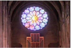
Figure 4. Rosette image tone mapped with Modified Simple Operator
Figure 5. Office image tone mapped with Simple Operator
Figure 6. Office image tone mapped with Modified Simple Operator
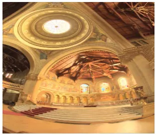
Figure 7. Stpeters_probe image tone mapped with Simple Operator
Figure 8. Stpeters_probe image tone mapped with Modified Simple Operator
Fact Findings and Observations from the results
It is found that Modified Simple Spatial Operator produces better images in terms of visual quality. As you can see in visual appearance of all images in the results (Figure 1 to Figure 8) that brightness is too much in images produce by Simple Spatial operator but Modified Simple Spatial Method reduces the excess brightness to produce better images and detail reproduction is better than Simple Spatial Operator and now the operator is fully automatic with no user parameter left. From the visual appearance of images it is clear that images produced with modified approach are better in quality.
2) Results based on quality metrics
We have implemented three quality metrics to assess the quality of images:
SSIM: It is Structural SIMilarity index metrics [9]. It compares the structures of two images reference image and the tone mapped image. Higher the value of SSIM is better the quality of produced image.
PSNR: It is Peak Signal to Noise Ratio. Higher the value betters the quality of produced image.
CPU Time (in secs): It is the time the particular algorithm takes to execute.
TABLEI SSIM COMPARISON
Images SSIM
Simple Modified Simple
Memorial 0.2093 0.2147
Nave 0.2054 0.2035
Rosette 0.9821 0.9832
Office 0.3801 0.4086
Stpeters_probe 0.6622 0.6626
TABLEIII
PSNR COMPARISON
Images PSNR
Simple Modified Simple
Memorial 38.0310 38.0454
Nave 19.9335 19.9338
Rosette 43.4621 43.5753
Office 50.7206 51.3861
Stpeters_probe 28.5426 28.5458
TABLEIIIII CPU TIME COMPARISON
Images CPU Time(in Secs)
Simple Modified Simple
Memorial 10.14 9.97
Nave 7.96 7.92
Rosette 2.9300 2.8547
Office 15.65 15.97
Stpeters_probe 63.35 63.47
Fact Findings and Observations from the results
From the values of quality metrics it is found that Modified Simple Spatial operator is better than the Simple Spatial operator. Like you can see the value of SSIM parameter is more in almost all cases except one “Nave” image in which
it comparable but PSNR parameter is better in each case and CPU time is also comparable and now the algorithm is fully automatic and user friendly.
V. CONCLUSIONS
In the end of the paper we would like to conclude that modified operator is better than the original operator as it produces better results in terms of quality metrics, visually and also make the operator fully automatic with no user parameter setting. After the analysis and survey we find that tone mapping is a key area for research. It requires more quality metrics which can assess the quality of image as human observer perceives and also it is found that no operator is perfect hence it is required to do modifications in the existing ones or to implement the new and better operators. Hence we find that tone mapping in HDR images is new and open area for research.
ACKNOWLEDGMENT
Thanks to Assistant Professor Sumeet Kaur for helpful discussions and to all who contributed high dynamic range data.
REFERENCES
[1] J. Tumblin and H. Rushmeier, “Tone Reproduction for Realistic Images,” IEEE Computer Graphics and Applications, vol. 13, no. 6, pp. 42-48, Nov. 1993.
[2] S.S. Stevens and J.C. Stevens, “Brightness Function: Parametric Effects of Adaptation and Contrast,” J. Optical Soc. Am., vol. 53, p. 1,139, 1960.
[3] Greg Ward, “A contrast-based scalefactor for luminance display,” In Graphics Gems IV, pages 415–421. Academic Press, Boston, 1994.
[4] Michael Ashikhmin, “A Tone Mapping Algorithm for High Contrast Images,” Eurographics Workshop on Rendering (2002). [5] E. Reinhard, M. Stark, P. Shirley, and J. Ferwerda, “Photographic
tone reproduction for digital images,” in Proc. of 29th annual Conference on Computer Graphics and Interactive Techniques, ACM SIGGRAPH, vol. 21, pp. 267–276, 2002.
[6] F. Drago, K. Myszkowski, T. Annen and N. Chiba, “Adaptive Logarithmic Mapping for Displaying High Contrast Scenes,” EUROGRAPHICS 2003.
[7] P. Ferschin, I. Tastl, and W. Purgathofer. “A comparison of techniques for the transformation of radiosity values to monitor colors,” In IEEE International Conference on Image Processing, volume 3, pages 992_996, 1994.
[8] K.K. Biswas and Sumanta Pattanaik, “A Simple Tone Mapping Operator for High Dynamic Range Images,” School of Computer Science, University of Central Florida; Orlando, Florida, 2005. [9] E. Reinhard, G. Ward, S. Pattanaik, and P. Debevec. High Dynamic
Range Imaging: Acquisition, Display, and Image-Based Lighting (The Morgan Kaufmann Series in Computer Graphics). Morgan Kaufmann Publishers Inc., 2005.
Sumandeep Kaur has 2 years of experience in software industry out of
which one year of experience is in image processing, has published one research paper in national level conference. Area of research is image processing.